


1. Introduction
Traditional loss reserving approaches in the property-casualty field produced a single point estimate value. Although no one truly expects losses to develop at exactly the stated value, the focus was on a single value for reserves that did not reflect the uncertainty inherent in the process. As the use of stochastic models in the insurance industry grew, for dynamic financial analysis (DFA), for asset liability management (ALM) and other advanced financial techniques, loss reserve variability became an important issue. McClenahan (2003) describes the history of interest in reserve variability and loss reserve ranges. Hettinger (2006) surveys the different approaches used to establish reserve ranges. The CAS Working Party on Quantifying Variability in Reserve Estimates (2005) provides a detailed description of the issue of reserve variability, including an extensive bibliography and set of issues that still need to be addressed. The conclusions of this Working Party are that despite extensive research on this area to date there is no clear consensus within the actuarial profession as to the appropriate approach for measuring this uncertainty, and that much additional work needs to be done in this area. All of the approaches described in this report, and suggestions for future research, focus on measuring uncertainty in statutory loss reserves. Given recent attention to fair value insurance accounting, future research should also focus on more accurate economic reserve ranges.
The use of nominal values for loss reserves is sometimes justified as providing a safety load, or risk margin, over the true (economic) value of the reserves. However, risk margins determined in this way would fluctuate with interest rates and vary by loss payout patterns. A more appropriate approach, which is beyond the scope of this research, would be to establish risk margins based on the risks inherent in the reserve estimation process, such as determining the risk margin based on the difference between the expected economic value and a level such as the 75th percentile value.
The Financial Accounting Standards Board (FASB) and the International Accounting Standards Board (IASB) have proposed an alternative approach to valuing insurance liabilities, including loss reserves. This approach, termed fair value, proposes that loss reserves in financial reports be set at a level that reflects the value that would exist if these liabilities were sold to another party in an arms length transaction. The relative infrequency with which these exchanges actually take place, and the confidentiality surrounding most trades that do occur, make this approach to valuation more of a theoretical exercise than a practical one, at least in the current environment. However, fair value would reflect the time value of money, so the trend would be to set loss reserves at their economic rather than nominal values if these proposals are implemented. The issues involved, and financial implications, in fair value accounting are covered extensively in the Casualty Actuarial Society report, Fair Value of P&C Liabilities: Practical Implications (2004). However, despite the comprehensive nature of the papers included in this report, little attention is paid to the impact the use of fair value accounting would have on loss reserve ranges. If reserves are to be calculated on a fair value basis, then reserve ranges should also be based on this approach as well.
A final impetus for this project is the recent criticism of the casualty actuarial profession over inaccurate loss reserves, and the profession’s response to these attacks. A Standard & Poor’s report (2003) blamed the reserve shortfalls the industry reported in 2002 and 2003 on actuarial “naiveté or knavery.” The actuarial profession responded strongly to this criticism, both with information and with investigation (Miller 2004). The Casualty Actuarial Society formed a task force to address the issues of actuarial credibility. The report of the Task Force on Actuarial Credibility (2005) included the recommendation that actuarial valuations include ranges to indicate the level of uncertainty in the reserving process, and that additional work be done to clarify what the ranges indicate. Once again, the focus was on statutory loss reserve indications, rather than the economic value.
The critical problem with setting reserve ranges based on nominal values is the impact of inflation on loss development. Based on relatively recent history (the 1970s) and current economic conditions (increasing international demand for raw materials, vulnerable oil supplies, the U.S. Federal Reserve’s response to the subprime credit crisis), increasing inflation has to be accorded some probability of occurring in the future by any actuary calculating loss reserve ranges. As inflation will affect all lines of business simultaneously, the impact of sustained high inflation would be to cause significant adverse loss reserve development for property-liability insurers. Loss reserve ranges based on nominal values would therefore include the high values that would be caused by a significant rise in inflation. However, inflation and interest rates are closely related, as first observed by Irving Fisher (1930) and confirmed by economists consistently since. The loss reserves impacted by high inflation would most likely be accompanied by high interest rates, so the economic value of those reserves would not be that much higher than the economic value of the point estimate for reserves. Using economic values to determine reserve ranges could also lead to narrower ranges and provide a clearer estimate of the true financial impact of reserve uncertainty.
This project utilizes realistic stochastic models for interest rates, inflation, and loss development to determine loss reserve distributions and ranges on both a nominal and economic basis, draws a comparison between the two approaches, and explains why the appropriate measure of uncertainty is based on the economic value. This work builds on prior work by Ahlgrim, D’Arcy, and Gorvett (2005) developing a financial scenario generator for the CAS and SOA as well as research on the interest sensitivity of loss reserves by D’Arcy and Gorvett (2000) and Ahlgrim, D’Arcy, and Gorvett (2004).
This study measures the uncertainty in loss reserving that is based on process risk, the inherent variability of a known stochastic process. In this analysis, both the distribution of losses and the parameters of the distributions are given. Thus, unlike actual loss reserving applications, there is no model risk or parameter risk. Setting loss reserves in practice involves more degrees of uncertainty and would therefore lead to greater variability in the underlying distributions of ultimate losses and larger reserve ranges. This study is meant to illustrate the difference between nominal and economic ranges, and starting with specified loss distributions more clearly demonstrates this effect.
2. Review of loss reserving methods
A primary responsibility of insurers is to ensure they have adequate capital to pay outstanding losses. Much research has been done on methods to evaluate and set these loss reserves. Berquist and Sherman (1977) and Wiser, Cockley, and Gardner (2001) provide excellent descriptions of the standard approaches used to obtain a point estimate for loss reserves. Loss reserve ranges became an issue in the past two decades, and has also been addressed in numerous papers. For example, Mack (1993) presented the chain-ladder estimates and ways to calculate the variance of the estimate. Murphy (1994) offered other variations of the chain-ladder method in a regression setting. Venter (2007) worked on improving the accuracy of these estimates and reducing the variances of the ranges. Other contributors to loss reserve estimates and discussions on the strengths and weaknesses of various evaluation models include Zehnwirth (1994), Narayan and Warthen (1997), Barnett and Zehnwirth (1998), Patel and Raws (1998), and Kirschner, Kerley, and Isaacs (2002). These works typically deal with nominal undiscounted value of loss reserves in line with statutory reserve requirements. Shapland (2003) explores the meaning of “reasonable” loss reserves, emphasizing the need for models to take into account the various risks involved along with “reasonable” assumptions. His paper points out that reasonableness is subject to many aspects, such as culture, guidelines, availability of information, and the audience; as such the paper concludes that more specific input is needed on what should be considered “reasonable” in the actuarial profession.
Traditional methods use embedded historical inflation to produce the nominal reserves. Outstanding losses will be exposed to the impact of inflation until they are finally paid. If the inflation rate during the experience period has been high, loss severity will be projected to be high generating large loss reserves. Similarly, after periods of low inflation, loss severity will be projected to increase more slowly, leading to lower loss reserves. Because inflation and interest rates are correlated, an insurer with an effective Asset Liability Management (ALM) strategy for dealing with interest rate risk can alleviate some of the impact of changing inflation.
There have been reserving techniques that attempt to isolate the inflationary component from the other effects, such as those proposed by Butsic (1981), Richards (1981), and Taylor (1977). Butsic investigated the effect of inflation upon incurred losses and loss reserves, as well as the inflation effect on investment income. For both increases and decreases in inflation, these components are found to vary proportionally. According to Butsic, as competitive pricing is dependent on a combination of both claim costs and investment income, insurers are to a large extent unaffected by unanticipated changes in inflation. Richards provides a simplified technique to evaluate the impact of inflation on loss reserves by factoring out inflation from historical loss data. Assumptions of future inflation can then be factored in to project possible values of future loss reserves. Under the Taylor separation method, loss development is divided into two components, inflation and superimposed inflation. This method assumes the inflation component affects all loss payments made in a given year to the same degree, regardless of the original accident year. Essentially, unpaid losses are not considered to be fixed in value over time but rather are fully sensitive to inflation. An alternative to this assumption is proposed by D’Arcy and Gorvett (2000), which allows loss reserves to gradually become “fixed” in value from the time of the loss to the time of settlement. Inflation would only affect the unpaid losses that have not yet become fixed in value. These two methods will be described in detail in the model section.
3. Asset liability management
Asset liability management (ALM) is a process in which organizations manage risk by considering the impact that an event would have on both their assets and their liabilities; risk is managed by using the offsetting effects to reduce aggregate risk to an acceptable level. For example, the fall of the dollar against the euro might increase the cost of claims an insurer would have to pay on business written in Europe. If the insurer held assets denominated in euros, then these would increase in value as the dollar fell, offsetting some, or all, of the increased claim costs. Although ALM can be used to deal with any type of financial risk, in practice most insurers focus on interest rate risk. In this context, if both assets and liabilities change by the same amount when interest rates rise or fall, there will be no interest rate risk for the firm. However, if they respond differently, the firm will be exposed to interest rate risk. Prior to the 1970s, mismatches between assets and liabilities were not a significant concern. Interest rates in the United States experienced only minor fluctuations, making any losses due to asset-liability mismatch insignificant. However the late 1970s and early 1980s were a period of high and volatile interest rates, making ALM a necessity for any viable financial institution. If interest rates increase, fixed income bonds decrease in value and the economic value (the discounted value of future loss payments) of the loss reserves decreases. The opposite occurs for both the assets and liabilities when interest rates decrease. Ahlgrim, D’Arcy, and Gorvett (2004) provide a detailed analysis of the effective duration and convexity of liabilities for property-liability insurers under stochastic interest rates that shows how assets can be invested to reduce the impact of interest rate risk.
Insurers can employ an ALM program to reduce the impact of inflation on loss reserves and maintain their surplus with changing interest rates. This requires insurers with short effective duration liabilities to hold short-term assets. Some insurers invest in longer duration assets that offer higher yields. During periods of stable or declining interest rates, this approach will provide a higher return. However, when interest rates rise this strategy can be costly.[1] The effect of duration mismatching on loss reserves given expectations of future inflation volatility is a complicated issue and is outside the scope of this paper. As will be shown later, the higher the correlation between nominal interest rates and inflation, such as in the 1970s, the more important and significant ALM’s impact will be.
4. Economic value of loss reserves
Recent developments by the Financial Accounting Standards Board (FASB) and the International Accounting Standards Committee (IASC) have advocated fair value accounting measures. The American Academy of Actuaries established the Fair Value Task Force to address this issue. The fair value of a financial asset or liability is its market value, or the market value of a similar asset or liability plus some adjustments. If a market does not exist, the asset or liability should be discounted to its present value at an appropriate capitalization rate depending on the risk components it encompasses. The Fair Value report by AAA (2002) provides details on the valuation principles. The promotion of fair value accounting, which considers both risk and the time value of money, indicates a new trend towards economic valuation.
The trend towards economic or market value based measurement of the balance sheet replacing existing accounting measures is also seen in the European Union, where solvency regulation is currently under reform. The European insurance and reinsurance federation, CEA (2007), describes how the new Solvency II project takes an integrated risk approach which will better account for the risks an insurer is exposed to than the current fixed standards under Solvency I. Solvency II introduces the use of a market-consistent valuation of assets and liabilities and market consistent reserve valuation, much like those proposed under fair value accounting in the United States.
Australian regulations have required ranges based on economic value since 1999. The value of the insurer’s liabilities is generally assumed to be independent of the insurer’s underlying assets. The Australian Prudential Regulation Authority’s “Audit and Actuarial Reporting and Valuation” (2006) and Institute of Actuaries of Australia Professional Standard 300 (2007) require loss reserves to be discounted by current observable market-based rates. These rates are based on characteristics of the future obligations, or derived from a yield of a replicating portfolio of low-risk securities. The study mentions that appropriate allowance can be made for future claim escalation from inflation and superimposed inflation (e.g. social or legal costs), but no clear methodology is provided as to how inflation should be taken into account.
Although there has been much discussion on the meaning of fair or economic value, both within and outside the United States, little attention has been given so far to the impact of economic value on loss reserve ranges. This paper ties together the loss reserve ranges with the economic values to show the relationship between loss reserve ranges on a nominal and economic basis and to illustrate some of the issues involved in calculating reserve ranges on economic values.
The economic value of an insurer’s liabilities is determined by discounting expected future cash flows emanating from the liabilities by their appropriate discount rate. Butsic (1988) and D’Arcy (1987) explore discounting reserves using a risk-adjusted interest rate which reflects the risk inherent in the outstanding reserve. Girard (2002) evaluates this using the company’s cost of capital. Actuarial Standard of Practice No. 20 (Actuarial Standards Board 1992) addresses issues actuaries should consider in determining discounted loss reserves. This standard suggests that possible discount factors could be the riskfree interest rate or the discount rate used in asset valuation.
5. Trends in inflation level and volatility
Inflation as measured by the 12-month change in the Consumer Price Index (CPI) has varied widely, from −11% to +20% over the period 1922 through 2007 (Figure 1). Since the adoption of Keynesian economic policies in developed countries following World War II, the general trend has been to avoid deflation at the cost of persistent inflation.[2] Rapid increases in oil prices in the 1970s and the early 21st century have increased inflation rates. The steady depreciation of the dollar in recent years has also put additional inflationary pressures on the U.S. economy. Recently, concern over the financial consequences of the subprime mortgage crisis and credit crunch has led the U.S. Federal Reserve to lower the discount rate to shield the economy from a housing slump and stabilize turbulence in the financial markets. Lowering interest rates is likely to lead to an increase in future inflation. Oil prices have risen sharply, the dollar has dropped to historical lows against the euro, and gold prices have soared. Falling prices of long-term government debt after the recent rate drop suggests investors concern over inflation. Thus, the potential for inflation to increase must be incorporated into any financial forecast.
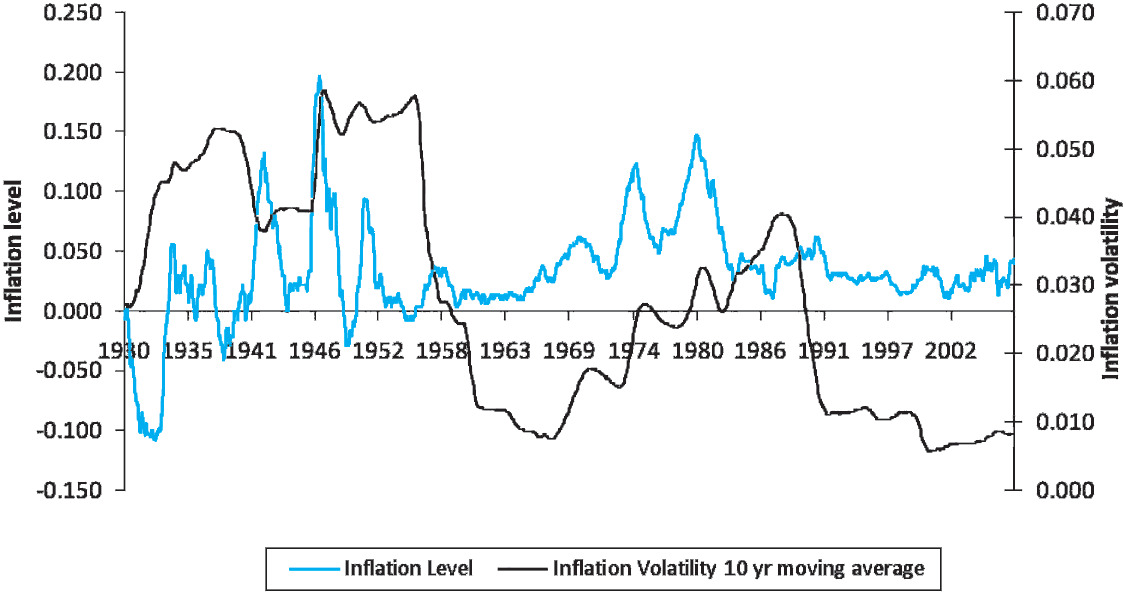
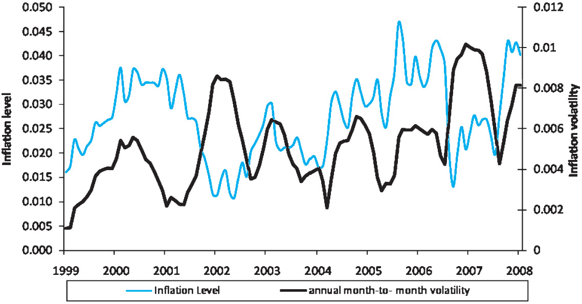
Figure 1 shows the inflation level and the inflation volatility (based on a 10-year moving average) since 1930. Inflation volatility, similar to interest rate volatility in interest rate models, is the standard deviation of the inflation rate over a one-year period. The 10-year moving average inflation volatility is calculated based on inflation rates over the last 120 months. The inflation rate is determined by the CPI at the end of each month compared to the CPI one year prior. Note the periods of deflation that occurred during the Depression and right after World War II, and the inflation spikes of the 1940s, 1950s, 1970s, and 1980s. Inflation volatility has also experienced several spikes, most recently in the 1980s. For the last decade, volatility has been at historic lows. Figure 2 shows the same data from the past 10 years, where there appears to be a rise in both inflation and inflation volatility. On this graph, inflation volatility is shown on a year-by-year basis (using only the last 12 months of data) to show the recent volatility more clearly. With the current upward trend in inflation volatility, it is necessary to consider the possibility inflation volatility returning to the levels of the 1950s or the 1980s. Inflation volatility determines how accurately we are able to predict future inflation trends; the greater the volatility, the lower the ability to forecast future inflation, and thus the greater uncertainty on its impact on loss reserves.
6. The models
The loss reserving model used in this research invokes: a loss generation model for loss severity, a loss decay model for loss payout patterns, a two-factor Hull-White model for nominal interest rates, an Ornstein-Uhlenbeck model for inflation, adjustment for correlation between the nominal interest rate and inflation, adjustment for claims cost inflation, and a fixed claims model for the impact of inflation on unpaid claims model. A sensitivity analysis worksheet is also built in to test the sensitivity of the parameters.
6.1. Loss generation model
The loss generation model generates aggregate claims based on the user’s input of the number of claims, choice of distribution of the claim severity, and the mean and standard deviation of severity. The number of claims is assumed to be known. The severity of claims can follow a Normal, Log-normal, or Pareto distribution.
6.2. Loss decay model
These losses can be settled either at a fixed time or at a rate based on a decay model over a number of years. If the claims are to be settled on a decaying basis, the decay model calculates the proportion of losses to be settled each year given a decay factor. For simplicity, loss severity is assumed to be independent of time to settlement. The decay model is of the following form:
Xt+1=(1−α)∗Xt
where Xi is the number of claims settled in year i, and α is the decay factor or the proportion of claims settled each year.
6.3. Nominal interest rate model
A two-factor Hull-White model is used to generate nominal interest rate paths. The Hull-White model uses a mean-reverting process with the short-term real interest rate reverting to a long-term real interest rate, which is itself stochastic and reverting to a long-term average level.
drt=κr(lt−rt)dt+σrdzrdlt=κl(μ−lt)dt+σldzl
where t is the time, r is the short-term rate, l is the long-term rate, κ is the mean reversion speed, µ is the average mean reversion level, dt is the time step, σ is the volatility, and dz is a Wiener process. This model allows for negative values, which is not theoretically possible for nominal interest rates. We impose a minimum short-term and long-term rate of 0% to adjust for this.
6.4. Inflation model
A one-factor Ornstein-Uhlenbeck model is used to generate inflation paths. The Ornstein-Uhlenbeck model uses a mean-reverting process with the current short-term inflation reverting to the long-term mean.
drt=κr(μr−rt)dt+σrdzr
where t is the time, r is the current inflation, κ is the mean reversion speed, µ is the long-term inflation mean, dt is the time step, σ is the volatility, and dz is a Wiener process.
6.5. Correlated nominal and real interest rates
The short-term nominal interest rate and inflation rates are correlated through their random shock components. The random dz component is adjusted for a weighted average between a common correlated random component and an individual random component.
dzr, nominal =ρdzcorrelated +√1−ρ2dznominal dzr, inflation =ρdzcorrelated +√1−ρ2dzinflation
where ρ is the correlation factor between the short-term interest rate and inflation rate, and dz are Wiener processes.
6.6. Masterson Claims Cost Index
Claim costs do not simply grow at the rate of inflation. The Masterson Claim Cost Index measures the rate at which claims costs are inflated over time by decomposing the costs into its various components and inflating each part separately (Masterson 1981, 1987; Van Ark 1996; Pecora 2005). For this research, the Masterson Claim Cost Index is simplified to a linear projection of the inflation rate.
6.7. Fixed claim model
Cash flows from unpaid claims are sensitive to inflation rate changes. Under the Taylor separation model (1977), any claim that has not been settled is subject to the full inflation in that year. If there is a car accident now and the claimant receives ongoing medical treatment for several years before the loss is settled, all medical costs are assumed to be impacted by inflation until the claim is paid. D’Arcy and Gorvett (2000) propose a model that reflects a different relationship between unpaid losses and inflation. Their model separates unpaid claims into portions that are “fixed” in value from those which are not. These fixed claims, once determined, will not be subject to future inflation while the remaining unfixed claims continue to be exposed to inflation. For example, medical treatment given over a period of time becomes fixed in value when the service is provided. If medical prices rise after some treatment has been provided, only future medical treatment will have this increased cost; medical treatment received before the price increase will have already been fixed. Any pain and suffering compensation is generally determined at a later date. This portion of the claim will likely continue to be affected by inflation until this claim is settled. As a result of only exposing partial loss segments to inflation, inflation’s impact on the loss is greatly reduced. A representative function that displays these attributes is:
f(t)=k+{(1−k−m)(t/T)n}
where f(t) represents the proportion of the ultimate claims “fixed” at time t, k is the proportion of the claim that is fixed immediately, m is the proportion of the claim that will be fixed only when the claim is settled, and T is the time at which the claim is fully settled.
The model (6.5) can be divided into three cases by the value of the exponent n: the linear case n = 1, when claim value is fixed uniformly up to its ultimate settlement; the convex case n > 1, when the rate of fixing the value of a claim increases over time, and the concave case n < 1, when the rate of fixing the value of a claim increases quickly initially but slows down as time approaches the ultimate settlement date. The larger the n, the more closely the fixed claim model will resemble the Taylor model.
7. Parameterization
Based on the 10-year loss development data of the auto insurance industry from A. M. Best’s Aggregate and Averages over the period 1980–1996, approximately one-half of all remaining losses of the total loss value are settled each year up to the ultimate settlement year. Assuming loss severity to be independent of time of settlement, we use a decay factor α = 0.5 for the number of claims settled each year. If loss severity is positively correlated with time of settlement, we would use a larger decay factor for the number of claims settled, but offset that by increasing the value of claims over time. Calculating the decay factor based on total loss value adjusts for the assumption that claims severity is independent of time to settlement.
Regressions were run against historical data to parameterize the Ornstein-Uhlenbeck inflation model and the two-factor Hull-White nominal interest rate model. These parameters are tabulated below:
The Fisher formula is an equilibrium statement that, on average, nominal rates and inflation are linked. Sarte (1998) has found that in an environment with stochastic inflation, the Fisher formula is still a reasonable approximation to its more complete counterpart in a dynamic endowment environment. It is also worthy to note that inflation is a matter of government policy rather than just a fact of nature; and the model should be adjusted to match the current economic situation.
The correlation between the three-month U.S. Treasury interest rates (the shortest securities issued) and percentage changes in the CPI index was determined for several periods as shown below. The relationship between inflation and interest rates hypothesized by Fisher applies to expected inflation and current interest rates. There is no reliable measure of expected inflation, so the actual inflation rate for a recent period is used here instead. The CPI is an estimate of a market basket of prices at a particular time; monthly changes include significant noise, as under- or overstated values in one month are adjusted the following month. This leads to the lowest values for the correlations. Inflation rates calculated based on three- and six-month CPI changes are more highly correlated with interest rates. The problem introduced by increasing the time period for determining the current inflation rate is that these rates may be less indicative of expected inflation. To run the model, we selected the one month inflation value over the more recent time period, or 45%. Other values for this correlation are shown in the sensitivity tests.
The Masterson Claims Cost Index for auto insurance bodily injury from 1936 to 2004 was regressed against the historical inflation rate using a fixed intercept of 0. The slope of the regression increases over time indicating that claim costs have been increasing more than CPI inflation benchmarks. A slope of 1.6 was selected for this model; other values are illustrated in the sensitivity section.
For the fixed claim model, we are using the linear case, with the parameter for k (portion of claim fixed at inception of claim) of 0.15 as suggested in D’Arcy and Gorvett (2000), but the parameter for m (portion of the claim fixed at settlement) at 0.5. The sensitivity of these values is examined in a later section.
8. Running the model
This model is available on the author’s website and will also be made available through the CAS website so any interested reader can run the model to reproduce the results here or test alternative parameters. The loss reserve model, which is designed in Microsoft Excel, begins with an input worksheet for the user to enter the parameters for each model used and the number of iterations to be made in the simulation. For each iteration, the model generates a loss distribution, a nominal interest rate path, and an inflation path, which are used to produce the nominal and economic loss ranges. An output worksheet collects the values from each iteration run and calculates the mean, standard deviation, and reserve ranges for both the nominal and economic value cases. The summary sheet collects these key statistics, the parameters used, and the number of iterations in the simulation in side-by-side columns for comparison.
The model is set to generate 1,000 random log-normally distributed claims settled on a decaying basis over 10 years. The mean and standard deviation of the losses are arbitrarily set to 1,000 and 250 respectively. The decay model then calculates the proportion of these claims settled at each time step up to the 10th year.
The generated losses are compounded at the inflation rate up to their time of settlement. This is the nominal, undiscounted value of losses that insurers are statutorily required to have as a reserve. The interest rate model generates cumulative interest rate paths corresponding to each time period up to settlement. The nominal values are then discounted back by this cumulative interest rate factor to obtain the economic value of losses.
For a simplified example, assume a single claim of $1,000 (based on the price level in effect when the loss occurred) is settled at the end of five years, and the annual nominal interest rate is 5%. Also assume that the inflation is equal to one half of the nominal rate throughout the five years, i.e., (1 + 5%)0.5 − 1= 0.0247. The nominal value of the loss reserve would be $1,000 * (1 + 2.47%)5 = $1129.73. This nominal value is discounted back by the interest rate over the five years to get the economic value $1129.73 * (1 + 5%)−5 = $885.17. In economic terms, the amount that should be reserved for handling this loss in today’s dollars is $885.17. Now consider what would happen if interest rates changed by 200 basis points up or down. If the nominal rate is 7%, inflation will be (1 + 7%)0.5 − 1 = 3.44%, and the nominal value and economic value will be $1,184.30 and $844.39, respectively. If the nominal rate is 3%, inflation will be (1 + 3%)0.5 − 1 = 1.49%, and the nominal value and economic value will be $1,076.70 and $928.77, respectively. Thus, the nominal value range will be $1,129.73 − $1,076.70 = $53.03, and the economic value range will be $928.77 − $885.17 = $43.60. The economic value range is only 82% of the nominal value range. This is a simplified example illustrating three possible values of one claim, assuming inflation is proportional to the nominal rate. Under circumstances like this, the reserve range based on economic values will be smaller than reserve ranges based on nominal values.
Now consider a book of 1,000 such claims and allow inflation to vary independently of nominal rates. The average nominal and economic values of these 1,000 claims are determined based on the interest rate and inflation paths generated for that simulation. This claims generation process is repeated for 10,000 simulations, with each simulation generating a different interest rate and inflation path for the 1,000 claims of that iteration, and a distribution of nominal and economic loss reserves are generated. The mean, standard deviation, minimum, maximum, as well as the 5, 25, 75, and 95 percentile for both the nominal and economic loss ranges are determined and compared. A confidence interval ratio is computed by dividing the economic range confidence interval by the nominal range confidence interval for both a 50 percent (ranging from the 25th percentile to the 75th percentile) and 90 percent (ranging from the 5th percentile to the 95th percentile) confidence interval. These ratios will be used as an indicator of the difference in volatility between the economic loss ranges and nominal loss ranges.
9. Results
To examine the effects of how the confidence interval is affected by changes in the assumptions, 10,000 simulations were run for each of the following cases. As the 50 percent and 90 percent confidence interval ratios turn out to be fairly close, only the 90 percent confidence interval ratios are shown here. The complete results are available from the authors. A monthly time step was chosen to provide a close approximation to continuous interest rate models, as inflation data are only available monthly.
9.1. Taylor Model versus Fixed Claim Model
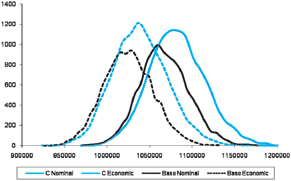
The first example is based on running the model with the following assumptions: 1) monthly time step, 2) a correlation factor of 45% between the nominal interest rate and inflation, 3) claims inflation rate of 1.6 times the general inflation rate, and 4) the Taylor separation model. This is Case A. Figure 3 shows the distributions for both the nominal and economic values; as would be expected, the economic values are lower than the nominal values, but the economic reserve range turns out to be approximately 94% of the nominal loss reserve range. Discounting does not reduce the ranges much. The second example, Case B, incorporates the fixed loss model suggested by D’Arcy and Gorvett (2000). In this case there is a significant decrease in the standard deviation of the nominal and economic reserves because losses are only partially exposed to inflation throughout its time to settlement. (Fixed claims are no longer affected by future inflation.) In this case the confidence interval ratio (the economic range divided by the nominal range) is 102%. Discounting reserves reduces the level of the reserves, but not the range. We will treat Case B as the base case and examine additional changes in relationship to this case. The mean values, standard deviations, 5th and 95th percentiles, and the 90% confidence intervals are for both nominal and economic values for Case A and Case B are shown on Table 1.
_vs._fixed_claim_(base_case__black).png)
9.2. High claims cost inflation
The relationship between claims inflation and the general inflation rate has varied widely over the period 1936 through 2004, but claims inflation is consistently higher than overall inflation. One reason for this is that medical costs are a major component of auto insurance claims and these have consistently outpaced general inflation. The third-party payer relationship also reduces resistance to cost increases, leading to higher inflation. Recently, the relationship between claims cost and inflation as increased significantly; between 2001 and 2004, auto bodily injury costs between increased 1.9 times the general inflation rate. For Case C, the claim cost inflation factor will be 1.9 and the standard deviation of the nominal range will be increased 1.9 times the original inflation volatility. As the nominal range is the claims cost inflated value of the real loss, higher claims cost inflation will increase the nominal range and decrease the confidence interval ratio. The distributions for both the Base Case and Case C are shown on Figure 4, and the key metrics of Case C are shown on Table 2. For Case C the confidence interval ratio of the economic range to the nominal range drops to 97%.
_vs._base_case_(black).png)
9.3. High correlation between inflation with nominal rates
Inflation and nominal interest rates moved in tandem during the 1970s, with correlation reaching 65% to 70%. Based on a 12-month inflation rate, the correlation with interest rates over the period 1970—2007 was 68%. High correlation between inflation and nominal interest rates reduces the range of economic loss reserves. For Case D the correlation factor was 70%. Figure 5 shows how this increase in correlation has little impact on the nominal values of loss reserves, but does reduce the distribution of economic values. In this case, the confidence interval ratio drops to 88% (Table 3).
_vs._base_case_(black).png)
9.4. Periods of high and volatile inflation
In the situation of high and volatile inflation, such as in the 1970s, the problem of using nominal loss reserves to determine reserve ranges is exacerbated. For Case E, the current inflation rate is increased to 10% (from the base case 3.54%) and the inflation volatility is increased to 6% (from 1.9%). Figure 6 shows how this change increases the level and range of the distribution compared with the base case. Table 4 provides the key metrics for Case E; the confidence intervals are much wider and the confidence interval ratio is 88%.
_vs._base_case_(black).png)
9.5. Summary of results
Based on the many simulations run for this research, the economic mean is smaller than the nominal mean. Under most circumstances, the economic value reserve ranges are slightly smaller than the nominal value ranges. This is not always the case under the fixed claim model. The economic value range will be smaller than the nominal value ranges if claims cost inflation is very high relative to the CPI inflation, if correlation is high between the nominal interest rate and inflation, or if inflation becomes highly volatile.
9.6. Sensitivity analysis
Sensitivity tests for all the parameters used were run to determine the impact of changes of each parameter. Case B was used as the base case, and each parameter was changed in turn over the ranges shown in Table 5. The results of a series of 5000 simulations of 1000 claims are summarized in the table below. For example, the first line of Table 5 indicates that changing the long run mean value for inflation over the range from 2% to 12% had no significant effect on the confidence interval range; in all cases, the economic value range was approximately 100% of the nominal value range. The next line indicates that changing the speed of mean reversion for the inflation rate over the range 0.1 to 0.3 increased the confidence interval range, in a linear manner, from 96% to 105%. Based on these results, the factors that have the most effect on the relationship between the confidence interval range of economic loss reserves and nominal loss reserves are the inflation volatility, the volatility of the short-term nominal interest rate, the correlation between interest rates and inflation, and the slope of the regression of claim costs against general inflation. These are the values that it is most important to measure accurately. A detailed discussion of the results for each parameter is provided in the appendix.
10. Conclusion
Property-liability insurance companies have traditionally valued their loss reserves on a nominal basis due to statutory requirements. These requirements do not reflect the economic value of the future payments and distort insurance company financial statements. Nominal loss reserves overstate the impact of inflation on reserves, though only slightly under the current economic environment, as they ignore the relationship between inflation and nominal interest rates. The economic impact on loss reserves of a change in inflation is commonly offset by a similar shift in the nominal interest rate and by the high claims cost inflation. Loss reserve ranges based on nominal values accentuate this problem. Recent proposals advocate the use of fair value accounting for loss reserves, which would replace nominal values with economic values. In this study a loss reserve model was developed to quantify the uncertainty introduced by stochastic interest rates and inflation rates and to compare reserve ranges based on nominal and economic values. The results demonstrate a variety of scenarios under which the reserve ranges based on economic values can be either smaller or larger than the nominal value ranges. However, use of economic values for loss reserves would better serve the insurance industry and its regulators. The key reason for encouraging the use of economic value ranges is that they properly reflect the true measure of the uncertainty involved in loss reserving. An additional benefit is that the ranges are smaller in many circumstances, and the current economic environment seems to be moving toward those situations. Claim cost inflation and the level and volatility of inflation appear to have an upward trend. Economic value reserves would provide more credible values of the cost and uncertainty of future loss payments, and in the cases mentioned before, would have a smaller confidence interval range.
Acknowledgment
The authors wish to thank the Actuarial Foundation and the Casualty Actuarial Society for financial support for this research.