Extreme Value Analysis for Partitioned Insurance Losses

1. Introduction

The heavy-tailed nature of insurance claims requires that special attention be put into the analysis of the tail of a loss distribution. Since a few large claims can significantly impact an insurance portfolio, statistical methods that deal with extreme losses have become necessary for actuaries. For example, in order to price certain reinsurance treaties, it is often necessary for actuaries to model losses in excess of some high threshold value, i.e., to model the largest k upper order statistics. Beirlant and Teugels (1992), McNeil (1997), Embrechts, Resnick, and Samorodnitsky (1999), Beirlant, Matthys, and Dierckx (2001), Cebrián, Denuit, and Lambert (2003), and Matthys et al. (2004) provide additional examples where statistical methods were developed to deal with extreme insurance losses.

Extreme value theory has become one of the main theories in developing statistical models for extreme insurance losses. The theory states that the tail of a typical loss distribution $F_X(x)$ can be approximated by a Pareto-type function. That is, $1-F_X(x)=\ell(x) x^{-\alpha}, x>D$ where $\ell: \mathbb{R}^{+} \rightarrow \mathbb{R}^{+}$ is a Lebesgue measurable function slowly varying at infinity, i.e., $\lim _{x \rightarrow \infty} \ell(t x) / \ell(x)=1$ for all $t>0$. The parameter $\alpha$ is known in the literature as the Pareto tail index that measures the heavy-tailedness of the loss distribution. See, for example, Finkelstein, Tucker, and Veeh (2006). Many distributions commonly seen in modeling insurance losses have Pareto-type tails. They include the Pareto, generalized Pareto, Burr, Fréchet, half T, F, inverse gamma, and log gamma distributions. Following the theory, an actuary may assume that the tail of the loss distribution, where extreme losses occur, can be approximated by a Pareto-type function without making specific assumption on the global density. With an estimate of the Pareto index parameter, the actuary can then estimate quantities of interest that are related to extreme losses, e.g., expected loss above a high retention limit. The approximation of a Pareto-type function has been demonstrated to be reasonable for many lines of insurance. Numerous tail index estimators have also been proposed in the literature, including earlier contributions by Hill (1975) and Pickands (1975) in which the Hill estimator has become somewhat of a benchmark to which later proposed estimators are compared. A survey of existing estimators, including their advantages and disadvantages, can be found in Brazauskas and Serfling (2000), Hsieh (2002), and Beirlant et al. (2004).

Insurance loss data reported in partitioned form are common in practice. The frequencies of losses occurred in certain loss intervals for numerous lines of insurance can often be found in companies’ reports or in government publications. Individual loss data are typically proprietary to the company and may not be available to its competitors in the industry. Despite the number of tail-index estimators proposed in the literature, many, if not all, of them require the use of individual loss data, and thus are inappropriate for tail-index estimation under the constraint of partitioned data. This paper intends to expand the horizon of tail-index estimation by applying extreme value theory to partitioned loss data. The main objective is to propose a robust tail-index estimator for partitioned loss data. The estimator is robust in the sense that no global density is assumed and the Pareto function is used to approximate the tail of a large class of distributions commonly used in modeling insurance loss data. This approach is advantageous because fitting a global density to losses can lead to errors when making tail inference in the event that the true loss distribution does not have the assumed density. Instead, we rely on the extreme value theory and focus only on fitting the tail of the distribution without assuming a specific global density. In addition, we will demonstrate the loss of efficiency by using the partitioned data versus individual data through simulation.

The remainder of the paper is arranged as follows. Several tail-index estimators are reviewed in Section 2. Except for the Hill and Pickands estimators, both of which have historical values, and the former serving as a benchmark in our simulation, the rest of the review is intended to be a supplement to the excellent reviews of Brazauskas and Serfling (2000), Hsieh (2002), and Beirlant et al. (2004). The derivation of the proposed estimator and an examination of its theoretical properties are worked out in Section 3. In Section 4, a simulation study is conducted to assess the performance of the proposed estimator. Two questions guide the design of the simulation: first, what is the efficiency lost by using data in partitioned form, and, second, what is the penalty of model misspecification? The simulation results are discussed in Section 5. Insurance applications are given in Section 6 using actual grouped insurance losses, followed by concluding remarks in Section 7.

2. Literature review

In this section we consider tail-index estimators for a loss random variable (r.v.) X taking values on the positive real line ℝ⁺ with nondegenerate distribution function F_X. We assume that the loss distribution has a Pareto-like tail in the sense that

$$\mathrm{P}(X>x)=\ell(x) x^{-\alpha}, \quad \text { as } \quad x \rightarrow \infty, \tag{2.1}$$

where $\alpha>0$. In this case the probability that a loss exceeds a level $x$ can be closely approximated by $C x^{-\alpha}$ when $x$ is larger than some threshold $D$. We will denote the tail probability function by $\bar{F}_X(x):=1-F_X(x)$. Let $\left\{X_k: 1 \leq\right. k \leq n\}$ be a sequence of independent copies of $X$ and denote the descending order statistics by $X^{(1)} \geq X^{(2)} \geq \cdots \geq X^{(n)}$.

In the following subsections, we discuss several estimators for the tail index α. Some noteworthy estimators that are not discussed below are the method of moments, probability-weighted moments, elemental percentile, Bayes estimator with conjugate priors, and hybrid estimators. A description of these can be found, for example, in Hsieh (2002) and the references therein.

2.1. The Hill and Pickands estimators

Hill (1975) proposed the tail-index estimator

$$\hat{\alpha}_{H}=\frac{k+1}{\sum_{i=1}^{k} i \log \left(\frac{X^{(i)}}{X^{(i+1)}}\right)} \tag{2.2}$$

based on a maximum likelihood argument where $k \in\{1,2, \ldots, n-1\}$. The Hill estimator is closely related to the mean excess function $e(u)=\mathrm{E}\{X- u \mid X>u\}$. In particular, the empirical mean excess function is given by $e_n(u)=\left[\operatorname{card} \Lambda_n(u)\right]^{-1} \sum_{j \in \Lambda_n(u)}\left(X_j-u\right)$, where $\operatorname{card} \Lambda_n(u)$ denotes the number of elements in the set $\left\{j: X_j-u>0, j=\right. 1, \ldots, n\}$. Then, letting $e_n^*(u)$ denote the empirical mean excess function of the log transformed variables, we have $e_n^*\left(\log X^{(k+1)}\right)=(1 / k) \sum_{i=1}^k \left(\log X^{(i)}-\log X^{(k+1)}\right)$. As a result, we see that $\hat{\alpha}_H=((k+1) / k) e_n^*\left(\log X^{(k+1)}\right)^{-1}$. That is, the Hill estimator is asymptotically equal to the reciprocal of the empirical mean excess function of $\log X$ evaluated at the threshold $\log X^{(k+1)}$.

An important feature of the Hill estimator to keep in mind is the variance-bias tradeoff that occurs when choosing the number of upper order statistics to use. Choosing too many of the largest order statistics can lead to a biased estimator, while too few increases the variability of the estimator. See Embrechts, Klüppelberg, and Mikosch (1997) for a further variance-bias tradeoff discussion and Hall (1990), Dekkers and De Haan (1993), Dupuis (1999), and Hsieh (1999) for methods for determining the number of upper-order statistics or threshold to use. Properties of the Hill estimator can be found in Embrechts, Klüppelberg, and Mikosch (1997) and the references therein.

Pickands (1975) proposed an estimator that matches the 0.5 and 0.75 quantiles of the generalized Pareto distribution (GPD) with quantile estimates. More specifically, for a GPD r.v. X with distribution function

$$G(x ; \xi, \sigma)=1-\left(1+\frac{\xi x}{\sigma}\right)^{-1 / \xi} 1_{(0, \infty)}(x)$$

it is easy to show that

$$\frac{G^{-1}(0.75)-G^{-1}(0.5)}{G^{-1}(0.5)}=2^{\xi} .$$

Then denoting 0.5 and 0.75 quantile estimates by q̂₁ and q̂₂, respectively, we have

$$\hat{\xi}=\frac{\log \left(\frac{\hat{q}_{2}-\hat{q}_{1}}{\hat{q}_{1}}\right)}{\log 2} .$$

Pickands proposed, for $n$ independent copies of $X$, using $\hat{q}_1=X^{(m)}-X^{(4 m)}$ and $\hat{q}_2=X^{(2 m)}-X^{(4 m)}$ where $n \gg m \geq 1$. Then noting that the tail index for a GPD r.v. is given by $\alpha=1 / \xi$, the resulting tail index estimate is, for $X^{(k)} \geq D$,

$$\hat{\alpha}_{P}=\frac{\log 2}{\log \left(\frac{X^{(m)}-X^{(2 m)}}{X^{(2 m)}-X^{(4 m)}}\right)} \tag{2.3}$$

where $k \geq 4 m \geq 4$.

For consistency and asymptotic results, see Dekkers and De Haan (1989). While the simplicity of the Pickands estimator is an attractive feature, it makes use of only three upper-order statistics and can have a large asymptotic variance. Generalized versions of the Pickands estimator can be found, for example, in Segers (2005). See Section 2.2.2.

2.2. Some recent tail-index estimators

2.2.1. Censored data estimator

In the case of moderate right censoring, Beirlant and Guillou (2001) proposed an estimator based on the slope of the Pareto quantile plot, excluding the censored data. This can be useful in situations when there has been a policy limit or when a reinsurer has covered losses in the portfolio exceeding some well-defined retention level. Letting N_c denote the number of censored losses, the estimator is

$$\hat{\alpha}_{N_{c}}(k)=\frac{k-N_{c}}{\sum_{i=N_{c}+1}^{k} \log \frac{X^{(i)}}{X^{(k+1)}}+N_{c} \log \frac{X^{\left(N_{c}+1\right)}}{X^{(k+1)}}}, \tag{2.4}$$

where k ∈ {N_c + 1, . . . ,n − 1}. This estimator is equivalent to the Hill estimator (except for the change from k + 1 to k, which is asymptotically negligible) in the case of no censoring (i.e., N_c = 0). It is argued by Beirlant and Guillou (2001) that typically no more than 5% of observations should be censored for an effective use of this method.

2.2.2. Location invariant estimators

It is pointed out by Fraga Alves (2001) that, for modeling large claims in an insurance portfolio, it is desirable for an estimator of α to have the same distribution for the excesses taken over any possible fixed deductible. For this reason, location invariance is clearly a desirable property for an estimator of α. Fraga Alves (2001) introduced a Hill-type estimator that is made location invariant by a random shift. The location-invariant estimator is

$$\hat{\alpha}_{k_{0}, k}=\frac{k_{0}}{\sum_{i=1}^{k_{0}} \log \frac{X^{(i)}-X^{(k+1)}}{X^{\left(k_{0}+1\right)}-X^{(k+1)}}}, \tag{2.5}$$

where $k_0$ is a secondary value chosen with $k_0<k$. An algorithm is included in Fraga Alves (2001) to estimate the optimal $k_0$, and to make a bias correction adjustment to $\hat{\alpha}_{k_0, k}$.

Generalized Pickands estimators described in Segers (2005) are also location invariant and are linear combinations of log-spacings of order statistics. In particular, let Ʌ denote the collection of all signed Borel measures λ on (0,1] such that

$$\begin{array}{c} \lambda((0,1])=0, \quad \int \log (1 / t)|\lambda|(d t)<\infty, \\ \text { and } \quad \int \log (1 / t) \lambda(d t)=1 . \end{array}$$

Then for λ ∈ Ʌ and 0 < c < 1, the generalized Pickands estimators are given by

$$\begin{aligned} \hat{\alpha}_{k}(c, \lambda)=( & \sum_{i=1}^{k}\left[\lambda\left(\frac{i}{k}\right)-\lambda\left(\frac{i-1}{k}\right)\right] \\ & \left.\quad \times \log \left(X^{(1+\lfloor c j\rfloor)}-X^{(i+1)}\right)\right)^{-1} . \end{aligned} \tag{2.6}$$

See Segers (2005) for examples using different measures λ and theoretical properties of the generalized Pickands estimators. See also Drees (1998) for a general theory of location and scale invariant tail-index estimators that can be written as Hadamard differentiable continuous functionals of the empirical tail quantile function.

2.2.3. Generalized median estimator

Brazauskas and Serfling (2000) proposed a class of generalized median (GM) estimators with the goal of retaining a relatively high degree of efficiency while also being adequately robust. The GM estimator is found by considering, for $X^{(k)} \geq D$ and $r \in\{2, \ldots, k\}$, the median of a kernel $h$ evaluated over all $\binom{k}{r}$ subsets of $X^{(1)}, \ldots, X^{(k)}$. The GM estimator is then given by

$$\hat{\alpha}_{r}=\operatorname{med}\left\{h\left(X^{\left(i_{1}\right)}\right), \ldots, h\left(X^{\left(i_{r}\right)}\right)\right\}, \tag{2.7}$$

where {i₁, . . . ,i_r} corresponds to a set of distinct indices from {1, . . . ,k}. Examples of kernels h, properties of the GM estimators, and comparison between the GM estimators and several other estimators can be found in Brazauskas and Serfling (2000).

2.2.4. Probability integral transform statistic estimator

Finkelstein, Tucker, and Veeh (2006) describe a probability integral transform statistic (PITS) estimator for the tail-index parameter of a Pareto distribution. They develop the PITS estimator through an easily understandable and sound probabilistic argument. The PITS estimator is shown to be comparable to the best robust estimators. Consider first a random sample of Pareto random variables $X_1, \ldots, X_n$, each with common distribution function $F(x)=1-(D / x)^\alpha$ for $x \geq D$ where $D>0$ is known and $\alpha>0$. Then defining

$$G_{n, t}(\beta)=\frac{1}{n} \sum_{i=1}^{n}\left(\frac{D}{X_{i}}\right)^{\beta t},$$

where t > 0, observe that

$$G_{n, t}(\alpha)=\frac{1}{n} \sum_{i=1}^{n} \bar{F}\left(X_{i}\right)^{t} \stackrel{\mathrm{~d}}{=}=\frac{1}{n} \sum_{i=1}^{n} U_{i}^{t}$$

where U₁, . . . ,U_n are i.i.d Uniform (0,1) random variables. Applying the Strong Law of Large Numbers yields

$$G_{n, t}(\alpha) \xrightarrow{\mathrm{p}} E\left(U_{1}^{t}\right)=(t+1)^{-1} .$$

Using the idea of method of moment estimation, the PITS estimator is the solution of the equation $G_{n, t}(\beta)=(t+1)^{-1}$. The tuning parameter $t>0$ is used to adjust between robustness and efficiency. See Finkelstein, Tucker, and Veeh (2006) for details. In the case D is unknown, one can consider

$$G_{n, t, k}(\beta):=\frac{1}{n} \sum_{i=1}^{k}\left(\frac{X^{(k+1)}}{X^{(i)}}\right)^{\beta t}$$

for k ∈ {1,2, . . . ,n − 1} and use the same approach to arrive at a PITS estimator for the tail index α.

3. Tail-index estimator for partitioned data

Let $\left\{X_k: 1 \leq k \leq n\right\}$ be a sequence of independent copies of a loss random variable $X$ satisfying (2.1). Suppose that losses are grouped into classes $\left\{I_i=\left(a_i, a_{i-1}\right]\right\}_{i=1, \ldots, g}$, where $\infty=a_0> a_1>\cdots>a_g>0$. Assuming the loss distribution has the Pareto-type form above a threshold $D$, we take $0<D \leq a_k$ without loss of generality for some $k \in\{2,3, \ldots, g\}$. We let $N_1, \ldots, N_g$ denote the frequencies with which $\left(X_1, \ldots, X_n\right)$ take values in $\left\{I_i=\left(a_i, a_{i-1}\right]\right\}_{i=1, \ldots, g}$. That is, $N_i= \operatorname{card}\left\{j: a_{i+1}<X_j \leq a_i, \quad 1 \leq j \leq n\right\}, \quad i=1, \ldots, g$.

The likelihood function is then defined as

$$L_{1}=\frac{n!}{\prod_{i=1}^{r} n_{i}!} \prod_{i=1}^{g}\left(\int_{a_{i}}^{a_{i-1}} f_{X}(x) d \mu(x)\right)^{n_{i}},$$

where f_X is the density of X with respect to Lebesgue measure μ. Hence

$$L_{1} \propto \prod_{i=1}^{g}\left(\bar{F}_{X}\left(a_{i}\right)-\bar{F}_{X}\left(a_{i-1}\right)\right)^{n_{i}}$$

Then setting $\bar{F}_X(x)$ equal to $\ell(x) x^{-\alpha}$ for $x \geq a_k \geq D$, we consider the conditional likelihood function $L\left(\alpha \mid n_1, \ldots, n_k\right)$ proportional to

$$\begin{aligned} L_{k}(\alpha) & =\prod_{i=1}^{k}\left(\frac{\bar{F}_{X}\left(a_{i}\right)-\bar{F}_{X}\left(a_{i-1}\right)}{\bar{F}_{X}\left(a_{k}\right)}\right)^{n_{i}} \\ & \approx \prod_{i=1}^{k}\left(\frac{a_{i}^{-\alpha}-a_{i-1}^{-\alpha}}{a_{k}^{-\alpha}}\right)^{n_{i}}, \end{aligned} \tag{3.1}$$

where $a_0^{-\alpha}$ is set to 0 . The proposed tail-index estimator is given by

$$G_{k}:=\arg \max L_{k}(\alpha) \tag{3.2}$$

where k ∈ {2,3, . . . ,g}. That is, G_k equals the value of α that maximizes the likelihood function L_k defined in Eq. (3.1). The lemma below shows that G_k exists and is a unique maximum likelihood estimator for α. As a result, one is able to obtain maximum likelihood estimates for tail probabilities and mean excess loss by using the invariance property of maximum likelihood estimators. These formulas are given in Section 6.

Lemma Existence and uniqueness of the proposed estimator

G_k in Eq. (3.2) exists and is unique.

Proof Define $b_i:=\log \left(a_i / a_k\right)$ for $i=1, \ldots, k$ and $u_i:=a_i / a_{i-1}$ for $i=2, \ldots, k$. Using Eq. (3.1), consider the log-likelihood function

$$\log L_{k}(\alpha)=\alpha n_{1} \log \left(a_{k} / a_{1}\right)+\sum_{i=2}^{k} n_{i} \log \left(\frac{a_{i}^{-\alpha}-a_{i-1}^{-\alpha}}{a_{k}^{-\alpha}}\right) .$$

Then it is easy to show using calculus that

$$\frac{\partial \log L_{k}(\alpha)}{\partial \alpha}=-n_{1} b_{1}-\sum_{i=2}^{k} n_{i}\left(\frac{b_{i}}{1-u_{i}^{\alpha}}+\frac{b_{i-1}}{1-u_{i}^{-\alpha}}\right) .$$

Noting that $u_i<1$ for each $i$ and $b_i>0$ for $i \geq 2$, we have

$$\frac{\partial \log L_{k}(\alpha)}{\partial \alpha} \longrightarrow\left\{\begin{array}{ll} -\sum_{i=1}^{k} n_{i} b_{i}<0, & \alpha \uparrow+\infty, \\ +\infty, & \alpha \downarrow 0 . \end{array}\right.$$

The result follows by noting that $b_i>b_{i-1}$ implies

$$\frac{\partial^{2} \log L_{k}(\alpha)}{\partial \alpha^{2}}=\frac{\left(b_{i}-b_{i-1}\right) \log u_{i}}{\left(2 \sinh \left(\alpha \log \left(u_{i}\right) / 2\right)\right)^{2}}<0 .$$

4. Performance assessment

In this section, we conduct a simulation to study the performance of the proposed tail estimator G_k. The two key questions guiding the design of the simulation are, first, what is the efficiency lost due to the use of partitioned data, and, second, how robust is the proposed estimator with respect to model misspecification?

Specifically, $m$ samples of size $n$ are generated from a distribution $F(x)$ with the mean $\mu<\infty$, standard deviation $\sigma$ and $x \geq 0$. The domain of $F(x), \mathbb{R}^{+}$, is partitioned into $g$ nonoverlapping intervals, $I_1, \ldots, I_g$. That is, $I_i \cap I_j=\varnothing$ for $1 \leq i \neq j \leq g$ and $\mathbb{R}^{+}=\cup_{i=1}^g I_i$. The individual observations in each sample are then grouped with respect to the partition, and frequencies $n_i$ in each interval, $i=1, \ldots, g$, are recorded. In this paper, we report the simulation results obtained from using $m=1000$ (samples), $n=1000$ (observations), $g=15$ (intervals), and the partition $I_i= \left(F^{-1}\left(p_i\right), F^{-1}\left(p_{i-1}\right)\right), \quad$ where $\left\{p_j\right\}_0^{15}=\{1.00$, $0.995,0.99,0.98,0.975,0.95,0.90$, (0.80, 0.70, $\ldots) 0.00\}$ for $i=1,2, \ldots, g$, and $F^{-1}(p)=\inf \{x$ : $F(x) \geq p\}$. We consider four distributions commonly used in modeling insurance losses. They include the Pareto with a parameter $\alpha$, generalized Pareto with parameters $\gamma$ and $\sigma$, Burr with parameters $\lambda, \theta$, and $\tau$, and the half T distribution with degrees of freedom $\phi$. The parameterizations of these distributions are given in Table 1.

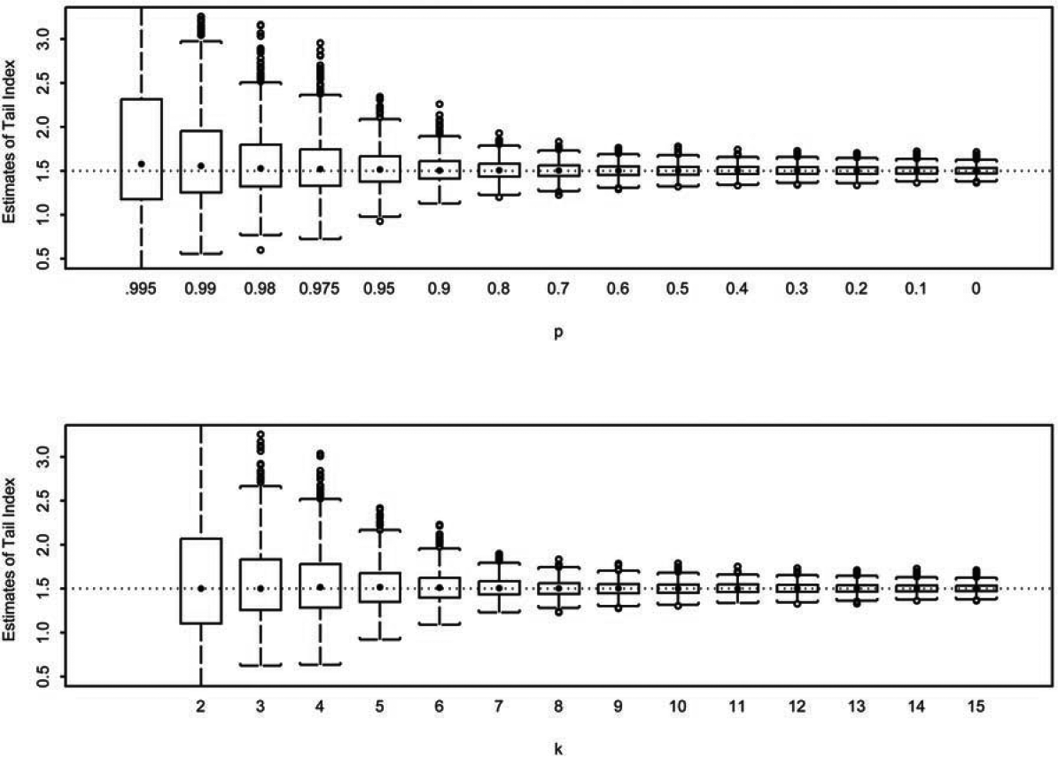
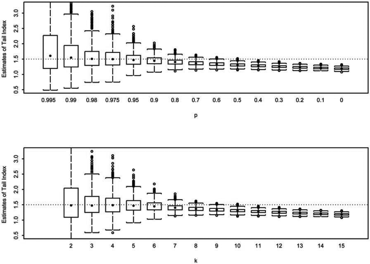
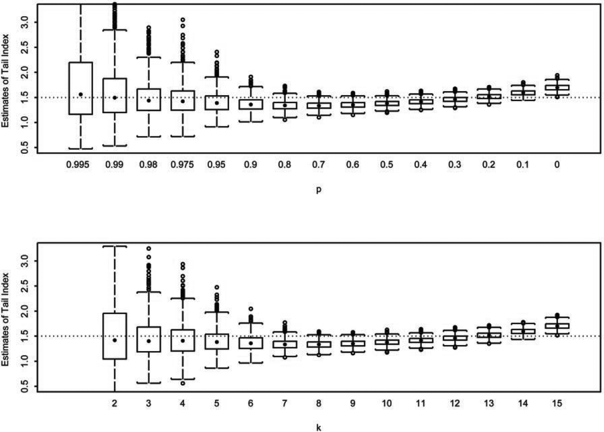
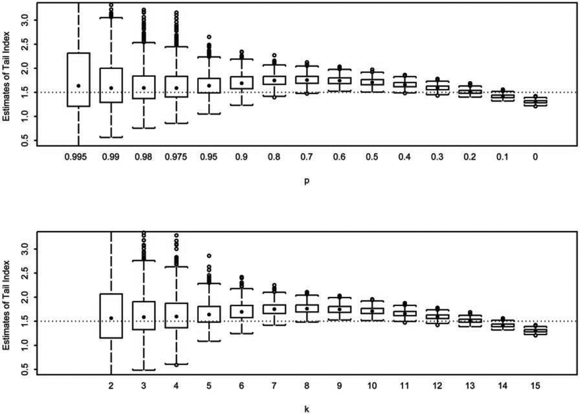
With simulated data in two different formats, the exact values as well as values in partitioned form, we compare the performance of the proposed estimator $G_k$ using frequencies in the intervals $I_i$ where $\inf I_i \geq D$ to that of the Hill estimator using all $x_i \geq D$, as well as to that of the maximum likelihood estimator using all frequencies $n_i$ or all $x_i$. In Figures 1-4, we report the loss in efficiency due to the use of partitioned data. The Hill estimates for $\alpha$ in the $j$ th box-plot, from left to right, are calculated using the largest $n_1+\cdots+n_j$ order statistics. The estimates from the proposed estimator in the $j$ th box-plot, from left to right, are calculated using Eq. (3.2) with $k=j+1$, for $j=1,2, \ldots, 14$. We notice that in Figures 1-4 the proposed estimator behaves similar to the Hill estimator. In addition, we take the tail estimates that comprise each box-plot to calculate the root mean squared error (RMSE). That is, for the $j$ th box-plot, $\mathrm{RMSE}_j= m^{-1} \sum_{i=1}^m\left(\hat{\alpha}_{j i}-\alpha\right)^2$, where $m=1000$, the true tail index $\alpha=1.50$, and $\hat{\alpha}_{j i}$ represents the $i$ th tailindex estimate in the $j$ th box-plot. The dashed line in each panel represents the true tail-index parameter value. To quantify the loss of efficiency, we further define efficiency (EFF) as the ratio of $\mathrm{RMSE}_j$ obtained from the proposed estimator to $\mathrm{RMSE}_j$ obtained from the Hill estimator. The results are reported in Table 2.

Figure 1.Performance of Hill (top) and $G_k$ (bottom) estimators for underlying Pareto model with true tail index $\alpha=1.5(D=1, \alpha=1.5)$. Hill estimates use all order statistics above $F^{-1}(p)$ where $F$ is the distribution function of the underlying distribution. Tail index estimates using grouped data are found using Eq. (3.2) for the given number of upper interval counts $k$. Sample size = number of replications = $1000$.

Figure 2.Performance of Hill (top) and $G_k$ (bottom) estimators for underlying generalized Pareto model with true tail index $\alpha=1.5(\gamma=1 / 1.5, \sigma=1)$. Hill estimates use all order statistics above $F^{-1}(p)$ where $F$ is the distribution function of the underlying distribution. Tail index estimates using grouped data are found using Eq. (3.2) for the given number of upper interval counts $k$. Sample size $\mathbf{=}$ number of replications $= 1 0 0 0$.

Figure 3.Performance of Hill (top) and $G_k$ (bottom) estimators for underlying Burr model with true tail index $\alpha=1.5(\lambda=1.2, \theta=4 / 2, \tau=3 / 4)$. Hill estimates use all order statistics above $F^{-1}(p)$ where $F$ is the distribution function of the underlying distribution. Tail index estimates using grouped data are found using Eq. (3.2) for the given number of upper interval counts $k$. Sample size $=$ number of replications $= 1000$.

Figure 4.Performance of Hill (top) and $G_k$ (bottom) estimators for underlying half T model with true tail index $\alpha=1.5(\phi=1.5)$. Hill estimates use all order statistics above $F^{-1}(p)$ where $F$ is the distribution function of the underlying distribution. Tail index estimates using grouped data are found using Eq. (3.2) for the given number of upper interval counts $k$. Sample size $=$ number of replications $= 1000$.

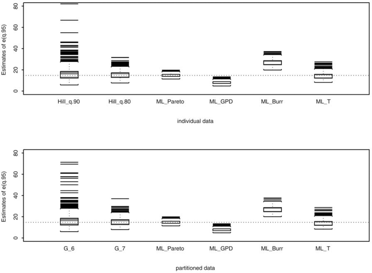
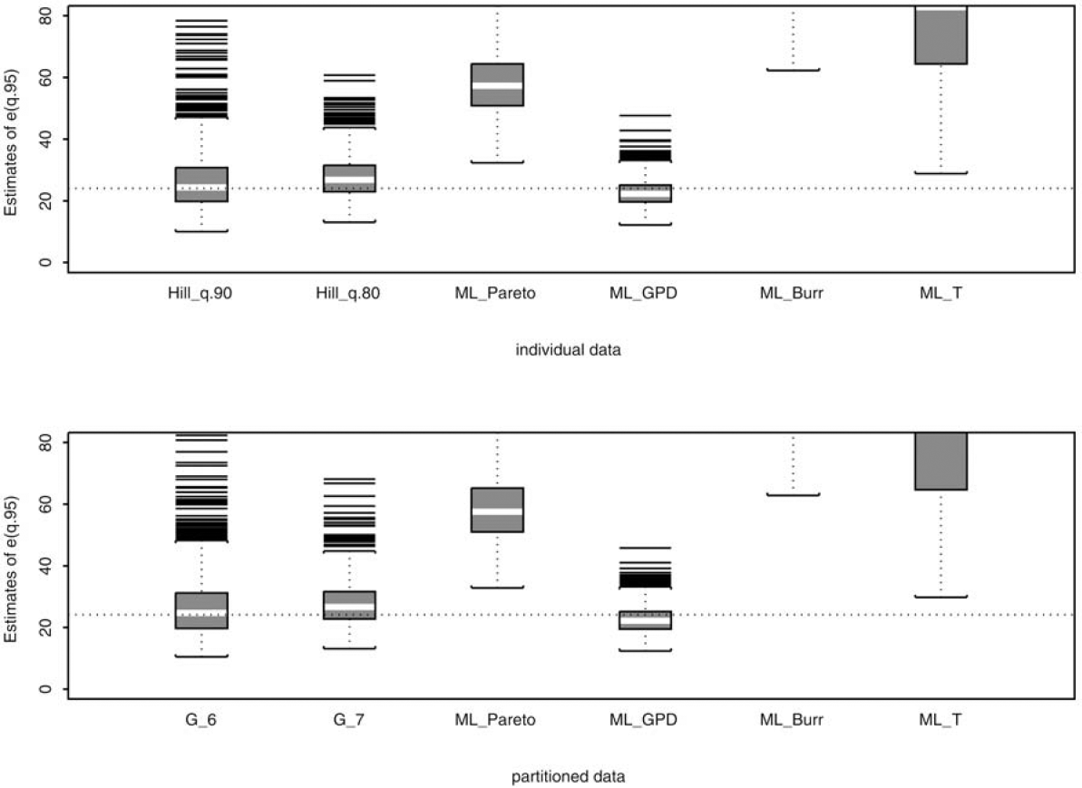
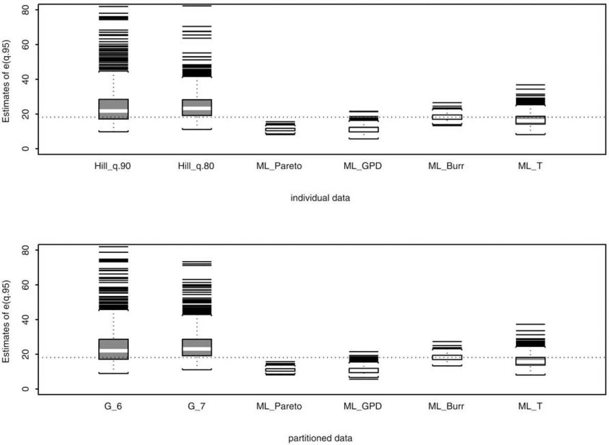
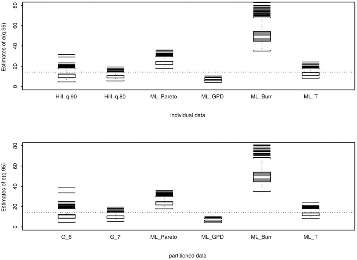
To examine the robustness of the proposed estimator against model misspecification, we compare the proposed estimator using frequencies in the top 6 and 7 intervals, which correspond to the 90th and 80th percentiles of the true underlying distribution, to four maximum likelihood (ML) estimators using all 15 frequencies N₁, . . . ,N₁₅. These four ML estimators differ in the assumed underlying distributions. They include Pareto (ML Pareto), generalized Pareto (ML GPD), Burr (ML Burr), and half T (ML T). Following our simulation design, it allows one of the four ML estimates to be the target estimate since this particular estimate is obtained by assuming the correct underlying distribution and by using the entire sample (all 15 frequencies) in estimation. The performance of the Hill estimator using observations above the 90th and 80th percentiles of the true distribution is also compared to those of the four similarly defined ML estimators that use the entire sample in estimation. With the tail estimates, we then calculate the expected loss exceeding the 95th percentile of the true distribution, e(q_.95) = E{X − q_.95 | X > q_.95}. The resulting expected losses are reported in Figures 5–8. In addition, we quantify these figures by calculating RMSE and EFF (see Table 3). Note that EFF in this table is defined as the ratio of RMSE of an estimator to that of the ML estimator that assumes the correct underlying distribution. Hence, if the true underlying distribution is Pareto, then EFF = 1 for ML_Pareto.

The simulation results for sample sizes 100, 250, and 500 are reported in the Appendix.

Figure 5.Estimation of mean excess value $e\left(q_{.95}\right)$. ML estimates are calculated under the assumption of the specified distributions. The true distribution $F$ is Pareto with tail index $\alpha=1.5$. The top plot uses all data, and the bottom plot uses grouped data. The Hill $q_{.90}$ and Hill $q_{.80}$ use all order statistics larger than $q_{.90}= F^{-1}(.90)$ and $q_{.80}=F^{-1}(.80)$. The $G_6$ and $G_7$ use the counts from top 6 and 7 intervals. Sample size = number of replications = 1000.

Figure 6.Estimation of mean excess value $e\left(q_{.95}\right)$. ML estimates are calculated under the assumption of the specified distributions. The true distribution $F$ is generalized Pareto with tail index $\alpha=1.5(\gamma=1 / 1.5, \sigma=1)$. The top plot uses all data, and the bottom plot uses grouped data. The Hill_ $q_{.90}$ and Hill_ $q_{.80}$ use all order statistics larger than $q_{.90}=F^{-1}(.90)$ and $q_{.80}=F^{-1}(.80)$. The $G_6$ and $G_7$ use the counts from top 6 and 7 intervals. Sample size $=$ number of replications $=1000$.

Figure 7.Estimation of mean excess value $e\left(q_{.95}\right)$. ML estimates are calculated under the assumption of the specified distributions. The true distribution $F$ is Burr with tail index $\alpha=1.5(\lambda=1.2, \theta=4 / 2, \tau=3 / 4)$. The top plot uses all data, and the bottom plot uses grouped data. The Hill $-_{9.90}$ and Hill $-q_{.80}$ use all order statistics larger than $q_{.90}=F^{-1}(.9)$ and $q_{.80}=F^{-1}(.8)$. The $G_6$ and $G_7$ use the counts from top 6 and 7 intervals. Sample size $=$ number of replications = 1000 .

Figure 8.Estimation of mean excess value $e\left(q_{.95}\right)$. ML estimates are calculated under the assumption of the specified distributions. The true distribution $F$ is half $\mathbf{T}$ with tail index $\alpha=1.5(\phi=1.5)$. The top plot uses all data, and the bottom plot uses grouped data. The Hill_ $q_{.90}$ and Hill_ $q_{.80}$ use all order statistics larger than $q_{.90}= F^{-1}(.9)$ and $q_{.80}=F^{-1}(.8)$. The $G_6$ and $G_7$ use the counts from top 6 and 7 intervals. Sample size = number of replications $=1000$.

5. Discussion of simulation results

The simulation conducted in the previous section illustrates the loss of efficiency in using partitioned data. There is no doubt that efficiency is lost with the use of partitioned data simply because fewer data points are used in maximizing the likelihood function. This is evident from those box-plots in the far left in Figures 1–4 and from the EFF measures in the first few columns in Table 2 when only observations exceeding the 95th percentile are used in estimation. For example, as shown in Table 2, when the underlying distribution is Pareto, the RMSE for the Hill estimator using observations exceeding the 99th percentile and the RMSE for the proposed estimator using the frequencies from the top two intervals are 0.75 and 4.47, respectively, giving EFF = 5.99. This implies that parameter estimation error, measured in RMSE, can be 5.99 times higher with the use of partitioned data than with the use of individual data. However, the amount of error quickly diminishes. With only the top three frequencies (N₁, N₂, and N₃) in use, the EFF is below 1.20 for all four distributions. Using the top five frequencies or more, the EFF never exceeds 1.10 and quickly approaches 1.01. The parameter estimation error between the use of partitioned data and of individual data becomes negligible.

The tables in Appendix A show results where sample sizes 500, 250, and 100 were used in the simulation. For n = 500, the EFF never exceeds 1.10 and quickly approaches 1.01 for all four distributions when the top five frequencies (i.e., upper 5%) are in use. This is similar to the findings with n = 1000. For n = 250, the top 6 (i.e., upper 10%), and for n = 100, the top seven frequencies (i.e., upper 20%) must be included for the EFF to go below 1.10. Our simulation seems to suggest that, for sample size between 100 and 1000, the loss of efficiency due to grouped data is minimal if 20% or more of the observations are included in estimating the tail index.

Figures 1–4 also reveal a typical problem in tail-index estimation. When taking only few data points in estimation, the resulting estimates exhibit large variance, whereas if taking more data points than necessary, the bias of the estimates seems evident. This variance-bias tradeoff suggests the development of a threshold selection process to determine a threshold above which the assumed Pareto-type functional form holds. In other words, we should not include any data points that are below the threshold in estimation to avoid bias because the assumed functional form is no longer valid. In addition to the diagnostic plot approach described in the next section, we may also consider an analytic approach to selecting the threshold for a given sample. We may start with the frequencies $N_1$ and $N_2$ in the first two intervals $I_1$ and $I_2$, and sequentially include frequencies in the adjacent intervals by testing whether the assumed functional form holds. We could perhaps make use of the fact that, conditional on $\sum_{i=1}^k N_i=\sum_{i=1}^k n_i, N_j \sim \operatorname{Binomial}\left(\sum_{i=1}^k n_i, p_{j k}(\alpha)\right)$, where $p_{j k}(\alpha)=\left(a_j^{-\alpha}-\right. \left.a_{j-1}^{-\alpha}\right) / a_k^{-\alpha}$. See, for example, Hsieh (1999) and Dupuis (1999).

If the underlying distribution is known, then the ML estimator is a common choice for parameter estimation. The ML estimate and the quantities derived from the estimate, e.g., the mean excess value e(u), possess desirable statistical properties. However, the true underlying distribution is typically unknown in practice, and the penalty of model misspecification and possibly subsequent misinformed decisions may not be negligible. Our simulation results shown in Figures 5–8 and in Table 3 illustrate the robustness of our proposed estimator and the penalty of model misspecification. It is clear from Table 1 that a reliable estimate of the tail index is crucial for estimating the mean excess function e(u). The estimation error of e(u) can be substantial without a reliable tail index estimator. For example, as reported in Table 3, when the true distribution is Pareto, the estimation error of e(u), measured as RMSE, for the four ML estimators using individual data and partitioned data ranges from 1.15 to 12.08, and from 1.16 to 12.09, respectively. ML_Pareto, not surprisingly, has the lowest RMSE because it assumes the correct underlying distribution and utilizes the entire sample. However, if the distribution is mistakenly assumed, then the RMSE can be 2, 6, or even 10 times higher than that of ML Pareto. In contrast, the RMSEs of the proposed estimator and the Hill estimator, despite using only a fraction of the data, stay relatively close to the best RMSE across all four assumed distributions, providing the robustness against model misspecification. The same conclusion can be drawn even with a sample size n = 100; see the tables in Appendix B.

Table 3 also highlights a problem often encountered in practice: the ML algorithm may not converge properly, leading to abnormal estimates. This is evident from the ML_Burr column where the ML algorithm did not converge in several iterations, resulting in insensible estimates, and thus, large RMSE.

Finally, the Hill and G_k estimators largely underestimate e(q_.95) when the true underlying distribution is half T (Figure 8). This is the result of the variance-bias tradeoff previously discussed. By using frequencies in the top 6 or 7 intervals, we have taken data from the area of distribution that the Pareto tail approximation does not hold. Once again, a threshold selection method is necessary to identify the optimal number k of frequencies to be used in G_k.

6. Applications to insurance

In this section we apply the proposed tail index estimator to actual insurance data available only in a partitioned form. The observed losses, summarized in Table 4, are taken from Hogg and Klugman (1984) and consist of Homeowners 02 policies in California during accident year 1977 supplied by the Insurance Services Office (ISO). Losses were developed to 27 months and include only policies with a $100 deductible.

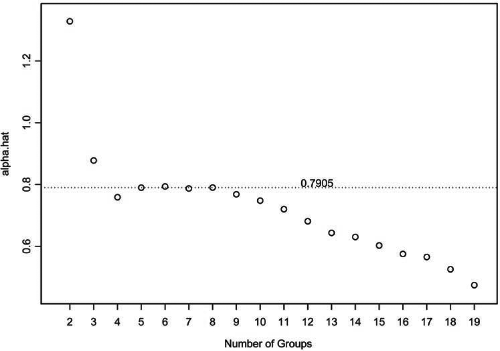
To determine the threshold above which to fit the Pareto tail and estimate the tail index, we look for a range in which the α estimates are stable. We use a plot similar to the Hill plot (see, for example, Embrechts, Klüppelberg, and Mikosch (1997) and Drees, de Haan, and Resnick (2000)), but modify it to be applicable for partitioned losses. Under our general framework, we consider the plot

$$\left\{\left(k, G_{k}\right): k=2, \ldots, g\right\}, \tag{6.1}$$

where k is the number of top groups used to find G_k, and look for a range of k values where the plot is approximately level. This plot is given in Figure 9 for the above insurance example. Notice that the plot is roughly linear for thresholds between 500 and 1100 (see also Table 4, 5 ≤ j ≤ 8). We use a_k := 500 (k = 8) as the thresh-old and obtain G_k = 0.7905. This tail index suggests no finite mean for the loss distribution.

Figure 9.Tail index estimation for fire loss data. The estimates for $\alpha$ using Eq. (3.2) are stable in the range $5 \leq k \leq 8$. This suggests to choose the cutoff $a_8=500$ as the threshold and to use the observed counts in top 8 intervals in Eq. (3.2).

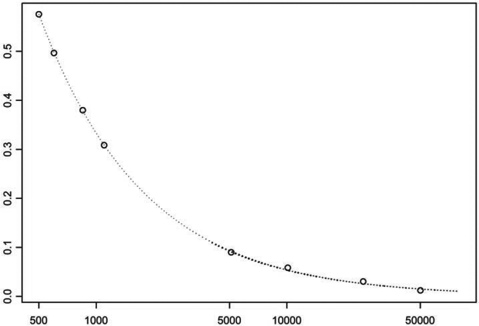
Next, we consider some important quantities in modeling large insurance claims, such as extreme tail probabilities, extreme quantiles, and mean excess loss, given that losses are available only in partitioned form. Under the setup described in Section 3, F (x)= P(X > x) can be approximated by

$$\hat{\bar{F}}(x)=\left\{\begin{array}{ll} \bar{F}_{n}\left(a_{k}\right)\left(x / a_{k}\right)^{-G_{k}} & \text { if } \quad x>a_{k} \\ \bar{F}_{n}(x) & \text { if } \quad x \leq a_{k}, \end{array}\right. \tag{6.2}$$

where F_n is the empirical d.f. for the losses X₁, . . . ,X_n. In Figure 10 this approximation is illustrated for the above Fire loss data with x > a_k = 500. Notice how closely the fitted tail probabilities are to the empirical tail probabilities.

Figure 10.Comparison of empirical and fitted tail probabilities for fire loss data. $\bar{F}_n(x)$ is given by open circles and $\hat{\bar{F}}(x)$ by the dashed line where $\hat{\alpha}=0.7905$ and $a_k=500$. Note that the $\mathbf{x}$ axis is on log scale.

Similarly, one can also approximate the conditional tail probability $\mathrm{P}\left(X>x \mid X>a_k\right)$ by $\left(x / a_k\right)^{-G_k}$. An extreme quantile of the loss distribution, $q_p$, is defined by the relationship $\bar{F}\left(q_p\right)= 1-p$ where $p$ is close to 1 (say, $F_n\left(a_k\right)<p<1$ ). Setting $\hat{\bar{F}}(x)$ equal to $1-p$ and solving for $q_p$ in Eq. (6.2) yields the following estimate for the extreme quantile $q_p$:

$$\hat{q}_{p}=a_{k}\left(\frac{1-p}{\bar{F}_{n}\left(a_{k}\right)}\right)^{-1 / G_{k}} \tag{6.3}$$

As an example, we estimate the .99 quantile to be $\hat{q}_{.99}=\$57,315$ using the above Fire loss data. The mean excess loss above a high threshold is important in premium determination and is given by $e(u)=\mathrm{E}\{X-u \mid X>u\}$. For $u>a_k$, the mean excess loss can be approximated by

$$\hat{e}(u)=\frac{u}{G_{k}-1}, \tag{6.4}$$

for $G_k>1$. In this example, however, $\hat{e}(u)$ is not available because $G_k \leq 1$.

7. Summary and conclusion

It has been shown that losses for many lines of insurance possess Pareto-type tails. For this reason, tail index estimation, which is a measure of the heavy-tailedness of a distribution, is an important problem for actuaries. Most estimators, however, cannot be used when loss data are available only in a partitioned form. The proposed estimator possesses the attractive features of (1) being applicable when loss data are available only in a partitioned form, and (2) being robust with respect to a large class of distributions commonly used in modeling insurance losses. We also showed that tail index estimates can be misleading if one misspecifies the distribution when trying to fit a global density. We have demonstrated that the proposed estimator compares favorably to the Hill estimator that uses individual data, and provided an example showing its effectiveness using actual insurance loss data.

Acknowledgments

The authors thank the financial support provided by the Committee on Knowledge Extension Research of the Society of Actuaries.