Parameterizing Payout Lag Time Distributions

undefined

1. Introduction

We want to consider the model of a claim with a random occurrence time followed by one payment after a random lag time. Our interest is in creating the distribution of payment lag time from occurrence. This distribution could best be estimated by having actual lag data for individual claims and then performing maximum likelihood estimation procedures on various distributions. However, actuaries typically do not have such data. Usually they have dollars or counts in the form of accident year by development year or by quarter, and sometimes policy year by development year. The payout information comes from estimating fractions of ultimate by development lag from the triangles of data and interpreting them as the probabilities of a cumulative distribution function. The aggregation of payment data is on the combined occurrence-payment process, which adds the two random times of occurrence and lag-to-payment to get the payout time.

The usual actuarial model of the claims process is that claims happen in the middle of the year and that payment activity happens only on anniversary dates of the claim; that is, immediately, exactly one year later, exactly two years later, and so on. The virtue of this model of the payout lag time distribution is that accident year by development year payout patterns are easy to fit. The payout density consists of a series of point masses on the anniversary dates, with the probabilities given directly by the aggregated data. Further, unless there are time-sensitive features in the problem, this may be adequate.

In this paper both the accident date and the lag to payment are modeled as continuous variables. One resulting advantage is that, given the payout lag distribution, we can work with partial years^[1] or switch to accident year by development quarter, or even accident year by development month if desired. It provides a natural way of interpolating empirical payouts and hence development factors. This representation allows one to use partial years of data at either end or even work with time periods of variable length. The technique also gives a consistent smoothing technique for payouts.

Section 2 develops the underlying formulas for arbitrary distribution density functions. Section 3 specializes to the particular class of distributions which are piecewise linear and continuous with a possible mass point at the origin. Details of much of the mathematics are relegated to the appendices.

Section 4 discusses the use of the formulas and the possible desirability of smoothing. The pay-out lag time distribution represents the combined activity of the claims departments, claimants, and sometimes courts. Our preference for the payout lag time density is a smooth curve with no zero values before the final tail.

Section 5 discusses how the companion spreadsheets are set up and how to use them. An example is given which uses excess layer Medical Malpractice (Med-Mal) data to illustrate the notions.

2. Probabilities and payouts

We denote by f(t) the probability density function for the lag time t of a payment for a claim occurring at time zero. We have the natural condition that f(t) = 0 for t < 0 (a claim is not usually paid before it occurs). Here, we assume that the density function for individual claim payment depends only on the time difference between occurrence and payment.^[2]

We denote the probability density function for occurrence at time t by occ(t). The occurrence distribution is assumed uniform but the equations could be modified to accommodate seasonality.^[3] Then the density for payment at time t is the convolution^[4] of these two densities:

$$p(t)=\int_{-\infty}^{t} \operatorname{occ}(x) f(t-x) d x. \tag{2.1}$$

Intuitively, this is the probability of an occurrence at time x multiplied by the probability of a payment at time t (lag of t − x), summed over available occurrence times. The probability of a payment between times a and b is

$$\begin{aligned} P(a, b) & =\int_{a}^{b} p(t) d t \\ & =\int_{a}^{b}\left\{\int_{-\infty}^{t} \operatorname{occ}(x) f(t-x) d x\right\} d t \\ & =\int_{0}^{\infty}\left\{\int_{a}^{b} \operatorname{occ}(t-z) d t\right\} f(z) d z. \end{aligned} \tag{2.2}$$

We may now frame the problem as follows: we have developed the probabilities of payment in various intervals (and ideally also their uncertainties^[5]) from some empirical payout pattern. We want to find a density function which is everywhere non-negative and closely gives the empirical payout pattern probabilities. We will supplement this in Section 4 by requiring that the density function also be reasonably believable.

We want the count payout pattern, but often have only a dollar payout pattern. If severities do not change over time then this is also the count payout pattern. However, it is often felt that larger claims close later, and in such a case we would have to find some way to approximate the count pattern. It may also be that the data is sufficiently noisy that it does not matter.

For accident-year data we take a uniform occurrence distribution between times 0 and 1. In Appendix A.2 the probability of seeing a payment in development year^[6] n = 0, 1, . . . is derived. Note that development year n begins at time n and ends at time n + 1.

$$\begin{aligned} P(n)= & \int_{n-1}^{n}(1+z-n) f(z) d z \\ & +\int_{n}^{n+1}(n+1-z) f(z) d z. \end{aligned} \tag{2.3}$$

The first term is, of course, missing^[7] for n = 0. The two terms represent the probabilities for a payment in calendar year n to come from payout year n − 1 or payout year n.

An alternative form of Equation (2.3) can be stated by using the cumulative distribution function (cdf)

$$F(x) \equiv \int_{0}^{x} f(z) d z \tag{2.4}$$

and the first moment cumulative distribution function

$$F_{1}(x) \equiv \int_{0}^{x} z f(z) d z. \tag{2.5}$$

We define the increments

$$\Delta(n) \equiv F(n+1)-F(n), \quad \text{and}, \tag{2.6}$$

$$\Delta_{1}(n) \equiv F_{1}(n+1)-F_{1}(n) . \tag{2.7}$$

We can also recognize that because of the generalized mean value theorem there is a quantity $\theta_n$ such that $0<\theta_n<1$ and

$$\Delta_{1}(n)=\left(n+\theta_{n}\right) \Delta(n) . \tag{2.8}$$

The specific form of $\theta_n$ will depend on the underlying density, of course. In Equation (A.16), Appendix A. 2 we derive the concise result

$$P(n)=\left(1-\theta_{n}\right) \Delta(n)+\theta_{n-1} \Delta(n-1) . \tag{2.9}$$

The equivalent and more directly usable form using cdf increments is

$$\begin{aligned} P(n)= & (n+1) \Delta(n)-(n-1) \Delta(n-1)-\Delta_{1}(n) \\ & +\Delta_{1}(n-1) \end{aligned} \tag{2.10}$$

for n ≥ 1 and

$$P(0)=\Delta(0)-\Delta_{1}(0) . \tag{2.11}$$

As an example, if the density is exponential $f(t)=e^{-t / \tau} / \tau$ with mean time $\tau>0$ then

$$\begin{aligned} F(n) & =\int_{0}^{n} e^{-z / \tau} / \tau d z=1-e^{-n / \tau} \\ \Delta(n) & =e^{-n / \tau}\left(1-e^{-1 / \tau}\right) \\ F_{1}(n) & =\tau\left[1-e^{-n / \tau}(1+n / \tau)\right] \quad \text { and } \\ \Delta_{1}(n) & =e^{-n / \tau}\left[(\tau+n)\left(1-e^{-1 / \tau}\right)-e^{-1 / \tau}\right] . \end{aligned}$$

For $n \geq 1, P(0)=1-\tau\left(1-e^{-1 / \tau}\right)$ and $P(n) =\tau e^{-(n-1) / \tau}\left(1-e^{-1 / \tau}\right)^2$. Note that $\theta_n=\tau- \left(e^{1 / \tau}-1\right)^{-1}$ is independent of $n$ and $0<\theta_n< 1 / 2$, which satisfies the general requirement $0<\theta_n<1$.

For accident-year data by development quarter, we change the meaning of the index n to refer to quarters. The occurrence distribution is uniform over n = 0, 1, 2, and 3 and a claim has probability 1/4 to be in any one of them. Let Q(n) be the probability for payment from an accident quarter in its development quarter n, conditional upon occurrence in that accident quarter. It will have the formulas of Equations (2.9) and (2.10). Let P(n) be the summed accident year by development quarter incremental probability. Then from Equation (A.21) in Appendix A.3 or just building up the accident year from quarters,

$$P_{Q}(n)=\sum_{k=\max (n-3,0)}^{n} Q(k) / 4 . \tag{2.12}$$

The factor 1/4 for each quarter comes from the accident-year occurrence density, as in Equation (A.20).

For policy year by development year, there is an additional step in the process. The policies are written over a year, and we will assume uniform writings, although again it is certainly possible to put in seasonal or other nonuniform behavior. After a policy is written, there is the distribution over time for a claim to happen up to a year later, which again we take to be uniform. The resulting claim occurrence density function is triangular and extends over two years in Equation (2.2). From Equation (A.25) in Appendix A.4, the probability of a payment in development year n is

$$\begin{aligned} P_{P Y}(n)= & \frac{1}{2} \int_{n}^{n+1}\left[(n+1)^{2}-2(n+1) z+z^{2}\right] f(z) d z \\ & +\int_{n-1}^{n}\left[1 / 2-n(n-1)+(2 n-1) z-z^{2}\right] f(z) d z \\ & +\frac{1}{2} \int_{n-2}^{n-1}\left[(n-2)^{2}-2(n-2) z+z^{2}\right] f(z) d z. \end{aligned} \tag{2.13}$$

For n = 0 only the first term is present, and for n = 1 only the first two. We will again express this in terms of the cumulative distribution functions, and because there is a quadratic term we will also need the differences of the second moment function:

$$F_{2}(x) \equiv \int_{0}^{x} z^{2} f(z) d z \tag{2.14}$$

$$\begin{aligned} \Delta_{2}(n) & \equiv F_{2}(n+1)-F_{2}(n) \equiv \int_{n}^{n+1} z^{2} f(z) d z \\ & \equiv\left(n^{2}+\phi_{n}\right) \Delta(n). \end{aligned} \tag{2.15}$$

The last equality defines $\phi_n$. Because of the mean value theorem, $0<\phi_n<2 n+1$ for any distribution. Then we may write

$$\begin{aligned} P_{P Y}(n)= & {\left[1 / 2-(n+1) \theta_{n}+(1 / 2) \phi_{n}\right] \Delta(n) } \\ & +\left[1 / 2+(2 n-1) \theta_{n-1}-\phi_{n-1}\right] \Delta(n-1) \\ & +\left[-(n-2) \theta_{n-2}+(1 / 2) \phi_{n-2}\right] \Delta(n-2) \end{aligned} \tag{2.16}$$

or the more directly useful form

$$\begin{aligned} P_{P Y}(n)= & \frac{1}{2}\left[(n+1)^{2} \Delta(n)-2(n+1) \Delta_{1}(n)+\Delta_{2}(n)\right] \\ & +\{[1 / 2-n(n-1)] \Delta(n-1) \\ & \left.+(2 n-1) \Delta_{1}(n-1)-\Delta_{2}(n-1)\right\} \\ & +\frac{1}{2}\left[(n-2)^{2} \Delta(n-2)-2(n-2) \Delta_{1}(n-2)\right. \\ & \left.+\Delta_{2}(n-2)\right] \end{aligned} \tag{2.17}$$

with

$$\begin{aligned} P_{P Y}(0)= & (1 / 2)\left[\Delta(0)-2 \Delta_{1}(0)+\Delta_{2}(0)\right] \\ P_{P Y}(1)= & {\left[2 \Delta(1)-2 \Delta_{1}(1)+(1 / 2) \Delta_{2}(1)\right] } \\ & +\left[(1 / 2) \Delta(0)+\Delta_{1}(0)-\Delta_{2}(0)\right] . \end{aligned} \tag{2.18}$$

3. A specific distribution

We will work in the context of the accident-year-by-development-year problem, but the extensions to the other cases are straightforward. The immediate question is how to get the payout lag time distribution given a payout pattern. We will pick a parameterized form of the density function and use it to develop formulas for the probabilities. There are, of course, many possible forms and the reader is certainly invited to create the probabilities of Equation (2.3) from her favorite form.

We will focus on a mixed distribution which has a possible positive probability at zero and a continuous distribution on positive time. A piecewise linear density function specifies values at the integer^[8] times and is linear between them. Mathematically, the form is

$$\begin{aligned} f(t)= & P_{0} \delta(t)+\sum_{n=0}^{N} I_{[n, n+1]}(t) \\ & \times\left[(n+1-t) f_{n}+(t-n) f_{n+1}\right]. \end{aligned} \tag{3.1}$$

We have switched from $x$ to $t$ as a variable to remind us that this is the time from occurrence to payout. The value $P_0$ is the amount of probability^[9] at $t=0$ and is subject to the constraint $0 \leq P_0 \leq 1$. It is meant to represent the probability of payout immediately after occurrence. The values $f_n$ are the values of the density function at times $t=n$. The interval function $I_{[n, n+1]}(t)$ is 1 in the interval $n \leq t \leq n+1$ and zero otherwise. The density function in that nonzero range has the value

$$(n+1-t) f_{n}+(t-n) f_{n+1} \tag{3.2}$$

which yields the straight line from $f_n$ at $t=n$ to $f_{n+1}$ at $t=n+1$. In order to be a probability density, we must have $f_n \geq 0$ for all $n$. Since our data is always bounded in time, we have specified $N+1$ intervals and we take $f_n=0$ for $n>=N+1$. However, if the reader knows of a good form for the tail she is encouraged to use it. For some patterns such as workers comp the distribution density almost certainly should be nonzero, well past any data we actually have.

Appendix B derives the results of the rest of this section. The differences of the cdf are

$$\begin{array}{l} \Delta(n)=\frac{f_{n}+f_{n+1}}{2} \quad \text { for } \quad n>0 \quad \text { and } \\ \Delta(0)=\frac{f_{0}+f_{1}}{2}+P_{0}. \end{array} \tag{3.3}$$

The cdf starts with P₀ and is quadratic in each interval. If K is the integer part of t and z is the fractional part of t so that t = K + z and 0 ≤ z < 1, then

$$F(t)=P_{0}+\sum_{n=0}^{K-1} \frac{f_{n}+f_{n+1}}{2}+\frac{z}{2}\left[(2-z) f_{K}+z f_{K+1}\right] . \tag{3.4}$$

If K = 0 the sum does not contribute. There is a constraint on the f_n in that the total probability must be 1:

$$1=F(N+1)=P_{0}+\frac{f_{0}}{2}+\sum_{n=1}^{N} f_{n} . \tag{3.5}$$

The accident-year-by-development-year probabilities of Equation (2.9) for n > 0 are

$$P(n)=\frac{f_{n-1}+4 f_{n}+f_{n+1}}{6} . \tag{3.6}$$

There are some special cases at both ends of the distributions:

$$\begin{aligned} P(0) & =P_{0}+\frac{2 f_{0}+f_{1}}{6} \\ P(N) & =\frac{f_{N-1}+4 f_{N}}{6} \\ P(N+1) & =\frac{f_{N}}{6} \\ P(n>N+1) & =0 . \end{aligned} \tag{3.7}$$

The accident-year-by-development-quarter probabilities from Equation (2.12) are generally

$$P_{Q}(n)=\frac{f_{n-4}+5 f_{n-3}+6 f_{n-2}+6 f_{n-1}+5 f_{n}+f_{n+1}}{24} . \tag{3.8}$$

The special cases at the start are from Equation (A.21),

$$\begin{array}{l} P_{Q}(0)=\operatorname{Pr}_{0}+\frac{2 f_{0}+f_{1}}{24} \\ P_{Q}(1)=\operatorname{Pr}_{0}+\frac{3 f_{0}+5 f_{1}+f_{2}}{24} \\ P_{Q}(2)=\operatorname{Pr}_{0}+\frac{3 f_{0}+6 f_{1}+5 f_{2}+f_{3}}{24} \\ P_{Q}(3)=\operatorname{Pr}_{0}+\frac{3 f_{0}+6 f_{1}+6 f_{2}+5 f_{3}+f_{4}}{24}, \end{array} \tag{3.9}$$

and the special cases at the end are

$$\begin{aligned} P_{Q}(N) & =\frac{f_{N-4}+5 f_{N-3}+6 f_{N-2}+6 f_{N-1}+5 f_{N}}{24} \\ P_{Q}(N+1) & =\frac{f_{N-3}+5 f_{N-2}+6 f_{N-1}+6 f_{N}}{24} \\ P_{Q}(N+2) & =\frac{f_{N-2}+5 f_{N-1}+6 f_{N}}{24} \\ P_{Q}(N+3) & =\frac{f_{N-1}+5 f_{N}}{24} \\ P_{Q}(N+4) & =\frac{f_{N}}{24} \\ P_{Q}(n) & =0 \quad \text { for } \quad n>N+4 . \end{aligned} \tag{3.10}$$

In practice it is easier just to use Equation (2.12) for the accident year as a sum of quarters.

The policy-year-by-development-year probabilities of Equation (2.16) are

$$P_{P Y}(n)=\frac{1}{24}\left(f_{n-2}+8 f_{n-1}+14 f_{n}+f_{n+1}\right) . \tag{3.11}$$

The special cases are similarly at the ends

$$\begin{array}{l} P_{P Y}(0)=\frac{\operatorname{Pr}_{0}}{2}+\frac{3 f_{0}+f_{1}}{24} \\ P_{P Y}(1)=\frac{\operatorname{Pr}_{0}}{2}+\frac{8 f_{0}+11 f_{1}+f_{2}}{24} \end{array} \tag{3.12}$$

and

$$\begin{aligned} P_{P Y}(N) & =\frac{f_{N-2}+8 f_{N-1}+14 f_{N}}{24} \\ P_{P Y}(N+1) & =\frac{f_{N-1}+8 f_{N}}{24} \\ P_{P Y}(N+2) & =\frac{f_{N}}{24} \\ P_{P Y}(n) & =0 \quad \text { for } \quad n>N+2 . \end{aligned} \tag{3.13}$$

4. Believability and smoothing

It is a fair question to ask why we have bothered with creating a continuous distribution for payout times. As mentioned in the introduction, the implicit accident-year-by-development-year payout distribution which is widely used is one where the density is nonzero only at a discrete set of points on the lag time axis. The virtue of this distribution is that it is easy to parameterize. If the payout pattern indicates X% of the claims are paid in year n, then we put a X% probability at t = n.

This discrete distribution requires that once a claim occurs, it either is paid immediately or is paid exactly on one of its anniversary dates. While special circumstances may suggest that some claim payments may cluster around anniversary dates, in general it not believable that claims never have payments at times other than anniversary dates.

The problem noted with this discrete distribution is twofold: its density has zero values almost everywhere, and it is not smooth. One expects the density to be smooth, however, because of the complexity of the process that actually produces a payment. We do not expect that there will be lag times with no probability of payment before the end of the tail.

We are trying to create a distribution over payment lag time that more closely reflects reality. We do not know exactly what this distribution should look like for any given line of business. The distribution could have a probability of (almost) immediate payment. The density should ultimately fall to zero. For some direct lines such as personal insurance, we might expect the density to decrease monotonically to zero. Alternatively, it may have a peak a few years out. For excess lines and reinsurance perhaps the density should rise from zero. There is some suggestion that workers comp claims may be bimodal because of short- and long-term care. Also, there may be enough of a distinction in some lines of business between claims that go to court and those that do not to create more than one peak.

In all cases, we do not expect there to be regions of zero probability before the final tailing out and we do expect the density to be smooth—the failure of both these requirements is what we find unreal about the discrete distribution.

What prejudgment on the density may or not be applied to results from available data is clearly a matter for the judgment of the actuary in any particular situation.

There is another reason for considering smoothing, which has to do with the noise in any data. Looking at the accident-year relations Equations (3.6) and (3.7), it would seem that for a finite amount of data we should just solve the equations. We certainly could. After all, we have N + 2 probabilities P(0) to P(N + 1) and we have N + 2 parameters in P₀ and f₀ to f_N. It is even a set of linear equations, and we can begin at the high end and work recursively backwards. This sounds good until it comes up against actual data. While it is true that mathematically the equations can be easily solved, what cannot be guaranteed is that all the parameters thus produced from real data^[10] are positive. If they aren’t, then we do not have an actual density function and we have to try something different.

Note that negative parameters in the density have nothing to do with negative payments; we are talking about the probabilities of having a payment and not about the payment size. If one has a line with considerable salvage and subrogation at the end of the payment pattern, it may be worthwhile to have the severity change sign at some point in time or create two densities, one for the positive payments and one for the negative. If the data are separate, just model sal-sub separately from the outgoing payments.

What can create negative parameters? Having data from not very many claims in the payout triangles; using average^[11] payout values and not recognizing the uncertainty associated with them; not really having a line of business where the payout pattern can be reasonably represented by only a single payment; having noise in the data from miscoding or other sources; any combination of the above; or something else. We do not expect to get negative parameters for payout patterns created by many claims in straightforward lines of business, but we want a procedure which will always work.

So what can we do? We can recognize that the data always has noise in it, and that a perfect fit may not even be desirable. Outliers do happen. We can pick some measure of fit—we used variance-weighted least squares error—and minimize the differences between the data and the predicted probabilities using normalized positive parameters. In other words, we can insist on a proper density function and see how close we can get. In the cases where we could solve the equations and get positive parameters, we will get the solution and in every case we have something physically consistent.^[12]

Experimentation with the spreadsheet tools has indicated that it is typically possible to get a pretty good fit, even to very irregular data. However, the cost to the best fit may be that the density function has violent swings in it, and possibly be zero over some periods. Neither of these properties is desirable, and we would like to have a way to ameliorate them.

The spreadsheets have as an input the weight to be given to having a smooth result. As this weight is increased from zero, the payout density function gets smoother–here meaning smaller changes in the slopes from segment to segment. However, the fit gets worse. The question of how much weight to give to the smoothing to get a more believable density function is purely subjective, and depends in part on how bad it is to be away from the exact values of the data points. If the data points have substantial intrinsic uncertainty, then considerable smoothing of the density may be possible with very little statistical loss of fit even though the predicted curve moves substantially.

It should be said that if smoothing is used, the density parameters will depend on the smoothness measure as well as on the degree to which the smoothness is imposed. The measure of smoothness used here, which seems to work well, is the sum of the squares of the differences of the slopes at each interior point in the distribution. This measure is zero when the density is a straight line and responds strongly to “W” shapes in the density. The reader is of course invited to use any smoothing measure that seems appropriate or none at all if it is not needed.

Since the predicted curve is derived from using a valid density, it smoothes—“graduates” in older terminology—the data in a consistent fashion. Frequently smoothing of the data is desirable in the first place and was often done on an ad hoc basis.

There is one further consideration. After doing the smoothing or not, the analyst may recognize the shape of the density function as being essentially gamma or Pareto or something similar. If so, it is generally preferable to work with fewer rather than more parameters and it would be good to go back and recalculate the probabilities in the intervals on the basis of the new form of the density. These calculations are easily done in terms of the cdf and first moment cdf differences with Equation (2.10).

5. Spreadsheet tools^[13]

We will work with “AY Payout Density.xls” as the exemplar, since the accident quarter and policy year are similar except for the detailed formulas in the probabilities. These differ in that for “AY Payout Density.xls” we use Equations (3.6) and (3.7), while for “AQ Payout Density.xls” we incorporate accident-quarter data via Equation (2.12). This is equivalent to using Equations (3.8) to (3.10) but is perhaps easier to understand. For “PY Payout Density.xls” we use Equations (3.11) to (3.13).

The sheet labeled “accident-year data” has its inputs in light blue. There is an input for the payout pattern, its name, and the relative uncertainty of the payouts. The fundamental measure of fit is the square of the difference between the fitted values and the data divided by the square of the uncertainty, and summed over all the data points. There is also an input for the weight to give to smoothing. At first, leave it at zero.

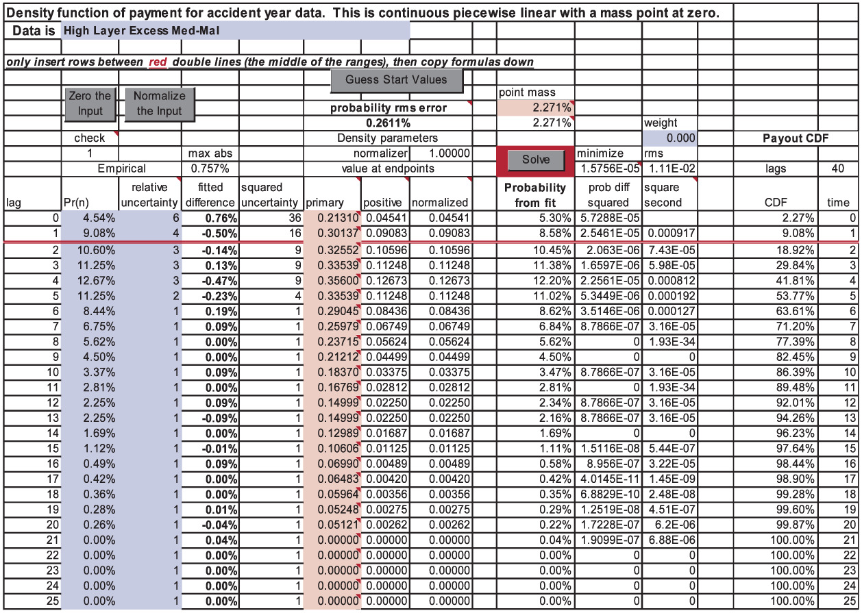
We begin by entering data. The data below is from some excess Med-Mal reinsurance contracts, but the uncertainties are estimated. Note that we have put in a relatively larger uncertainty for the earlier values.^[14] The button “Guess Start Values” puts half of the first data value (at n = 0) into the probability at zero, and puts the probabilities at each n as the estimate for fn. In the other spreadsheets there are modifications from these formulas made to the first few cells.

After clicking on “Guess Start Values” the data sheet “accident year data” looks in part as in Figure 1.

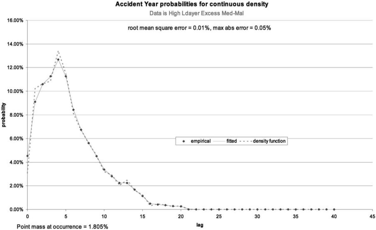
The graph sheet “AY probabilities” then shows Figure 2.

The graph’s horizontal axis has two meanings: for the data and the fit, it is the development period. For the density function, it is the lag from occurrence. At the guessed startup values the density function will follow the payout pattern and add a point mass at zero. The fit here is already not too bad.

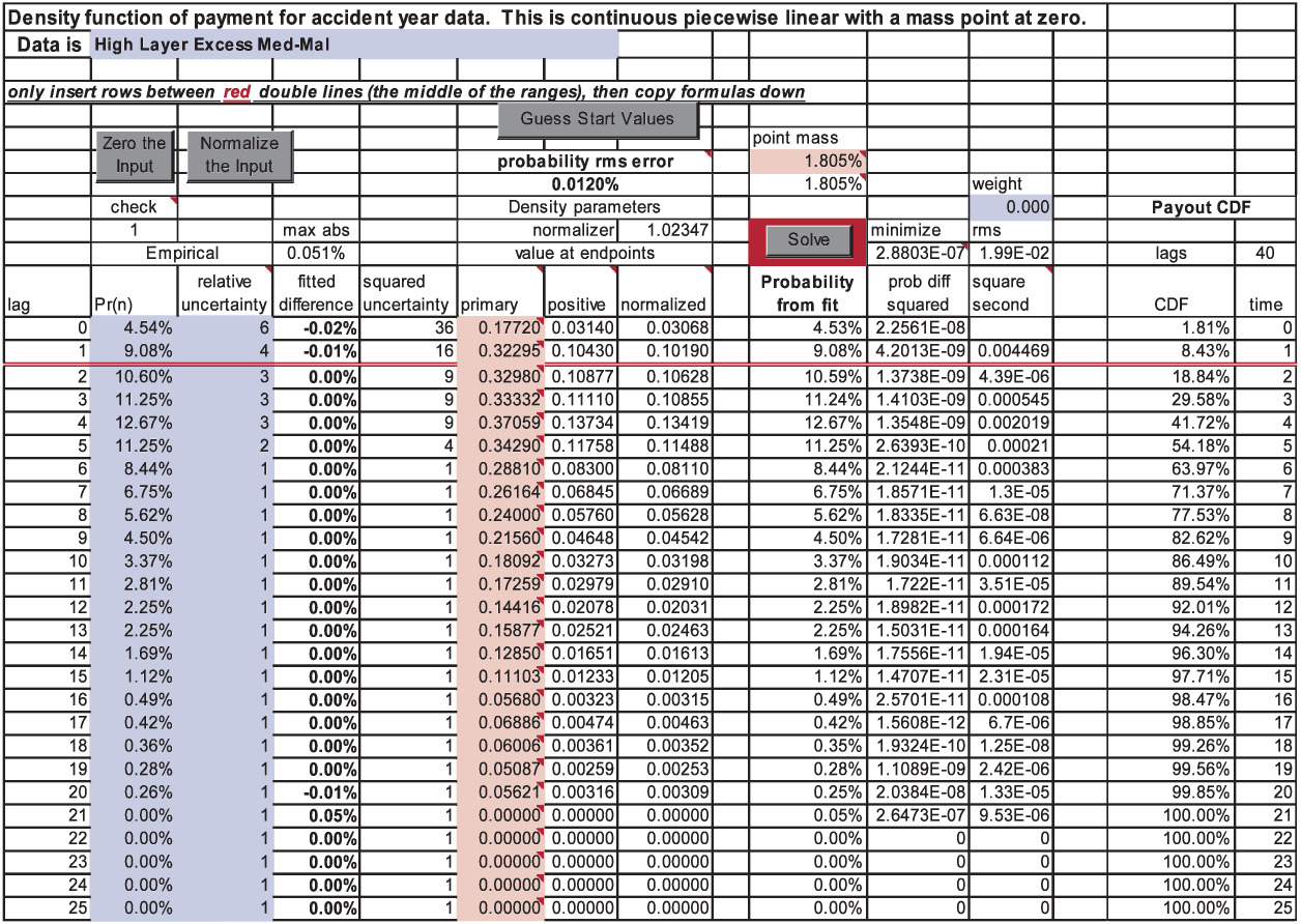
The next step is to run Excel Solver by clicking on “Solve.” This will vary all the density parameters to try to improve the fit. On the spreadsheet, the solver variables are allowed to vary freely, with the positivity constraints being imposed by formula rather in Solver itself. After Solver stops, the graph sheet shows Figure 3.

We can see from the error statistics that the fit is better. The root mean square error has decreased from 0.26% to 0.01% and the maximum absolute error has decreased from 0.76% to 0.05%. One could simply stop here and declare oneself satisfied. The data sheet now shows as in Figure 4.

Some notes for the data sheet: the input ranges can be extended by inserting rows between the two sets of double red lines^[15] and copying formulas down. This insures that the special conditions at both ends are met and all the named ranges retain their integrity. There are several convenience buttons: “Zero the Input” clears out old input; “Normalize the Input” multiplies it all by a factor to make its sum one; and “Guess Start Values” will usually give a reasonable place to begin the minimizations. As used above, “Solve” will run Excel Solver^[16] to minimize the criterion of fit. The cells in pink, also commented as “solver variable” are parameters changed by Solver.

The column “normalized value at endpoints” is directly the f_n of this paper. The column “Probability from fit” is our P(n). The columns labeled “Payout CDF” are the cdf values of the payout density and the corresponding lag time values. If we were working with noninteger time values, then this is where we would make the change, and consequently also on the sheet “CDF draw” to be discussed later. The data sheet gives the minimization function value, the root mean square (RMS) error, and the maximum absolute error for the fit. The latter two are also shown on the graph sheet.

The decision function minimized is the standard weighted least squares function plus a user-specified weight times the sum of the column labeled “square second.” As mentioned in the last section, each cell in that column is proportional to the square of the difference in slopes of the density at that point (which would be the second derivative), and has value zero if the density is a straight line. The effect of giving more weight to this column is to smooth out the density with most emphasis on the largest changes in slope.

The recommended use is to start with zero smoothing weight and observe the graph sheet. As you gradually increase the weight the density will become more and more smooth and the fit will worsen. In Figure 3, we might not like the shoulder between lags 2 and 4 and the very high value at lag 5, preferring a smoother variation of the underlying payout density. This is entirely a matter of actuarial judgment. With a smoothing value of 0.001, the graph sheet becomes as shown in Figure 5. The fit is not particularly worse, and the payout density is much more reasonable to the author’s perspective. It still has a very sharp peak at lag 5 and a wiggle at lags 12 and 13.

If we push the smoothing up to 0.05, we get Figure 6. Whether this fit is unacceptably bad depends on what we think the uncertainties are on the data, and especially in this case on how much we really believe the spike in the data at lag 5. This parameterization certainly does smooth out the payout lag time density function. The suggestion is to find a compromise that you can believe.

A word of caution: Solver will sometimes hang up in less than optimal solutions. The author’s recommendation is always to start with the “Guess Start Values” and put in the smoothing weight, and then “Solve.”

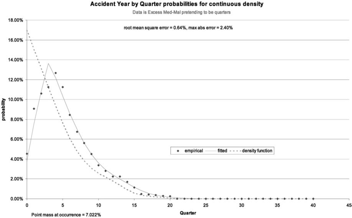
In the spreadsheet “AY by Q payout density.xls” the same accident-year data is used, while pretending that it is quarterly data instead. The best fit shows up as in Figure 7. This is a clear candidate for smoothing. A weight of 0.1 gives Figure 8. This still has zero probability values, so we try a weight of 1, yielding Figure 9. Since the data is unreal, it is perhaps not surprising that much smoothing was required.

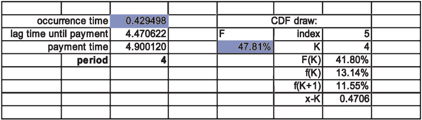
Finally, as a check on what the selected cdf for the payout will produce in simulation probabilities, the sheet “CDF draw” uses the cdf on the data sheet and the Equations (B.21) and (B.24) to illustrate how the random draws generate absolute time values for payouts. This sheet shows exactly how this payout is simulated in a timeline formulation. There is a random draw for the time of occurrence, and then another random draw from the cdf for the lag time from occurrence to payment. These two random times are added together, and then the integer part of their sum is the payment period. If you push F9 (Calculate) on this sheet you will see the process. The calculation part of the sheet looks like Figure 10. Again, the shaded cells are random uniform variables from the interval zero to one.

The button “Simulate” on this sheet will erase current data on the sheet “simulation results” and create new data for comparing the simulation with the predicted fit of “Probability from fit.” This is provided in case one wants to validate the formulas, and also is a reminder that a finite number of simulations will usually give a mean result near but not at the theoretical value.

Appendix

Appendix A. Mathematical derivations

A.1. Accident-year probabilities

There are undoubtedly much more concise derivations of the results presented here. However, we have used the same methodology everywhere in this appendix and have written this version out in detail so that the reader will hopefully be able to follow the steps easily.

To aid in deriving Equation (2.3) from a uniform occurrence distribution and Equation (2.2), we first define the index function and list some of its properties:

$$\Theta(x)=\left\{\begin{array}{lll} 1 & \text { for } & x>0 \\ 0 & \text { for } & x<0 \end{array}\right\} . \tag{A.1}$$

This is the unit step function at zero. A useful and intuitive way to read a factor of Θ(x − a) is to say that “x must be greater than a.” This function has some obvious properties (up to a set of measure zero):

$$\Theta(x)=1-\Theta(-x) . \tag{A.2}$$

If x is greater than a and x is greater than b, then x is greater than the larger of the two. If a is greater than b, then x is greater than a, but if b is greater than a, then x is greater than b. Thus

$$\begin{array}{l} \Theta(x-a) \Theta(x-b) \\ =\Theta(x-\max [a, b]) \\ =\Theta(x-a) \Theta(a-b)+\Theta(x-b) \Theta(b-a) . \end{array} \tag{A.3}$$

Similarly, for “less than” relationships,

$$\begin{aligned} \Theta(a-x) \Theta(b-x)= & \Theta(\min [a, b]-x) \\ = & \Theta(a-x) \Theta(b-a) \\ & +\Theta(b-x) \Theta(a-b) \end{aligned} \tag{A.4}$$

$$\Theta(x-a) \Theta(a-x)=0 \tag{A.5}$$

$$\Theta(x-a) \Theta(b-x)=\Theta(x-a) \Theta(b-x) \Theta(b-a) . \tag{A.6}$$

Equation (A.3) and (A.4) will be particularly useful later on in formal manipulation of integrals. In fact, it is often helpful to make all integration limits infinite and put the finite limits into indicator functions. For example, $\int_a^{\infty} f(x) d x= \int_{-\infty}^{\infty} \Theta(x-a) f(x) d x$.

We can now state the uniform occurrence time density, which is 1 in the interval 0 ≤ t ≤ 1 and zero elsewhere, as

$$\operatorname{occ}(t)=\Theta(t) \Theta(1-t) . \tag{A.7}$$

A change of variable gives occ(t − z)= Θ(t − z) · Θ(1 − t + z), to be used immediately.

For the accident-year case with b > a using Equation (2.2) the probability for a payment in the interval can be developed. First we state the probability with the index functions:

$$\begin{aligned} P(a, b)= & \int_{a}^{b}\left\{\int_{0}^{\infty} \Theta(t-z) \Theta(1-t+z) f(z) d z\right\} d t \\ = & \int_{0}^{\infty}\left\{\int_{a}^{b} \Theta(t-z) \Theta(1-t+z) d t\right\} f(z) d z \\ = & \int_{0}^{\infty}\left\{\int_{-\infty}^{\infty} \Theta(t-a) \Theta(b-t) \Theta(t-z)\right. \\ & * \Theta(1+z-t) d t\} f(z) d z. \end{aligned} \tag{A.8}$$

Then we use Equation (A.3) on Θ(t − a)Θ(t − z) and Equation (A.4) on the other pair:

$$\begin{aligned} P(a, b) & =\int_{0}^{\infty} \int_{-\infty}^{\infty}\left\{\begin{array}{c} {[\Theta(t-a) \Theta(a-z)+\Theta(t-z) \Theta(z-a)]} \\ *[\Theta(b-t) \Theta(1+z-b)+\Theta(1+z-t) \Theta(b-1-z)] \end{array}\right\} d t f(z) d z \\ & =\int_{0}^{\infty} \int_{-\infty}^{\infty}\left\{\begin{array}{c} \Theta(t-a) \Theta(a-z) \Theta(b-t) \Theta(1+z-b) \\ +\Theta(t-a) \Theta(a-z) \Theta(1+z-t) \Theta(b-1-z) \\ +\Theta(t-z) \Theta(z-a) \Theta(b-t) \Theta(1+z-b) \\ +\Theta(t-z) \Theta(z-a) \Theta(1+z-t) \Theta(b-1-z) \end{array}\right\} d t f(z) d z . \end{aligned} \tag{A.9}$$

Finally, integrating out t gives

$$\begin{array}{l} P(a, b) \\ \quad=\int_{0}^{\infty}\left\{\begin{array}{c} (b-a) \Theta(a-z) \Theta(1+z-b) \\ +(1+z-a) \Theta(1+z-a) \Theta(a-z) \Theta(b-1-z) \\ +(b-z) \Theta(b-z) \Theta(z-a) \Theta(1+z-b) \\ +\Theta(z-a) \Theta(b-1-z) \end{array}\right\} f(z) d z \end{array} \tag{A.10}$$

This is the form that can be used for nonintegral or varying-sized time periods. See Section A.5 for an example where the last period is incomplete. In fact, we can use it for any set of time intervals over which the data happen to be stated.

A.2. Accident year by development year

Here a = n and b = n + 1 so the probability of payment in lag n ≥ 1 is

$$\begin{aligned} P(n) & =\int_{0}^{\infty}\left\{\begin{array}{c} \Theta(n-z) \Theta(z-n) \\ +(1+z-n) \Theta(1+z-n) \Theta(n-z) \Theta(n-z) \\ +(n+1-z) \Theta(n+1-z) \Theta(z-n) \Theta(z-n) \\ +\Theta(z-n) \Theta(n-z) \end{array}\right\} f(z) d z \\ & =\int_{0}^{\infty}\left\{\begin{array}{c} (1+z-n) \Theta(1+z-n) \Theta(n-z) \\ +(n+1-z) \Theta(n+1-z) \Theta(z-n) \end{array}\right\} f(z) d z. \end{aligned} \tag{A.11}$$

The first and last terms are zero because of Equation (A.5). Finally,

$$\begin{aligned} P(n)= & \int_{n-1}^{n}(1+z-n) f(z) d z \\ & +\int_{n}^{n+1}(n+1-z) f(z) d z. \end{aligned} \tag{A.12}$$

This is Equation (2.3). For the first lag, n = 0, only the second term contributes:

$$P(0)=\int_{0}^{1}(1-z) f(z) d z. \tag{A.13}$$

We can get an intuition for Equation (A.11) by looking at the second line of Equation (A.8) and realizing that we want to integrate t over the intersection of the intervals n ≤ t ≤ n +1 and z ≤ t ≤ z + 1. The four cases z > n + 1, n < z < n + 1, n − 1 < z < n, and z < n − 1 are the four terms in Equation (A.11). The first and last contribute zero, because the intersection does not exist. In the more general Equation (A.10) we have the same four terms.

In order to formulate in terms of the cumulative distribution functions $F(x) \equiv \int_0^x f(z) d z$ and $F_1(x) \equiv \int_0^x z f(z) d z$, we repeat the definitions in Equations (2.6) to (2.8):

$$\Delta(n) \equiv F(n+1)-F(n) . \tag{A.14}$$

$$\Delta_{1}(n) \equiv F_{1}(n+1)-F_{1}(n) \equiv\left(n+\theta_{n}\right) \Delta(n) . \tag{A.15}$$

We can restate Equation (A.12) for n ≥ 1 as

$$\begin{aligned} P(n)= & (1-n)[F(n)-F(n-1)]+\left[F_{1}(n)-F_{1}(n-1)\right] \\ & +(n+1)[F(n+1)-F(n)]-\left[F_{1}(n+1)-F_{1}(n)\right] \\ = & (1-n) \Delta(n-1)+\Delta_{1}(n-1)+(n+1) \Delta(n)-\Delta_{1}(n) . \end{aligned} \tag{A.16}$$

This is Equation (2.10). This can also be written

$$\begin{aligned} P(n)= & (1-n) \Delta(n-1)+\left(n-1+\theta_{n-1}\right) \Delta(n-1) \\ & +(n+1) \Delta(n)-\left(n+\theta_{n}\right) \Delta(n) \\ = & \theta_{n-1} \Delta(n-1)+\left(1-\theta_{n}\right) \Delta(n). \end{aligned} \tag{A.17}$$

This is Equation (2.9). When n = 0,

$$\begin{aligned} P(0) & =F(1)-F_{1}(1)=\Delta(0)-\theta_{0} \Delta(0) \\ & =\left(1-\theta_{0}\right) \Delta(0). \end{aligned} \tag{A.18}$$

A.3. Accident year by development quarter

The index is now taken to mean the quarter. The accident-year occurrence density is uniform in the range 0 ≤ t ≤ 4 and must integrate to 1, so we have

$$\begin{aligned} \operatorname{occ}(t) & =(1 / 4) \Theta(t) \Theta(4-t) \\ & =(1 / 4) \sum_{n=0}^{3} \Theta(t-n) \Theta(n+1-t) . \end{aligned} \tag{A.19}$$

The second form simply expresses that the accident year is a sum of four accident quarters. Let $Q(n)$ be the probability for payment in a quarter by one accident quarter. The formulas are either of Equations (A.12) or (A.16). Let $P_Q(n)$ be the summed accident year by development quarter incremental probability. Then, using the second form of Equation (A.19), we see that we have Equation (2.12):

$$P_{Q}(n)=\sum_{k=\max (n-3,0)}^{n} Q(k) / 4 . \tag{A.20}$$

Another way of writing this is to show the first three explicitly, which also shows the growth of the accident year:

$$\begin{aligned} P_{Q}(0) & =Q(0) / 4 \\ P_{Q}(1) & =(Q(0)+Q(1)) / 4 \\ P_{Q}(2) & =(Q(0)+Q(1)+Q(2)) / 4 \\ P_{Q}(n \geq 3) & =\sum_{k=n-3}^{n} Q(k) / 4 . \end{aligned} \tag{A.21}$$

A.4. Policy year by development year

In order to get the probability of claim occurrence as a function of time, we need to specify how policies are written and how claims occur for a policy. Let w(t) be the probability density for writing a policy at time t and h(t) the probability density for a claim to happen at time t from the onset of the policy. We explicitly assume that h(t) does not depend on the policy issuance time. We also assume that the policies are written uniformly in the year, and that the probability of a claim occurrence is uniform in the policy period. If other conditions are known, then they can be incorporated into the convolution. Using Equations (A.3) and (A.4) produces

$$\begin{aligned} \operatorname{occ}(t)= & \int_{-\infty}^{t} w(x) h(t-x) d x \\ = & \int_{-\infty}^{\infty} \Theta(x) \Theta(1-x) \Theta(t-x) \Theta(x+1-t) d x \\ = & \int_{-\infty}^{\infty}\left\{\begin{array}{c} {[\Theta(x) \Theta(1-t)+\Theta(x+1-t) \Theta(t-1)]} \\ *[\Theta(1-x) \Theta(t-1)+\Theta(t-x) \Theta(1-t)] \end{array}\right\} d x \\ = & \Theta(1-t) \int_{-\infty}^{\infty} \Theta(x) \Theta(t-x) d x \\ & +\Theta(t-1) \int_{-\infty}^{\infty} \Theta(1-x) \Theta(x+1-t) d x \\ = & t \Theta(t) \Theta(1-t)+(2-t) \Theta(2-t) \Theta(t-1). \end{aligned} \tag{A.22}$$

This result is the familiar triangular exposure curve rising from zero at t = 0 to 1 at t = 1 and falling to zero again at t = 2.

The probability for payment at time t between t = n and t = n + 1 is again given by Equation (2.2).

$$\small{ \begin{aligned} P_{P Y}(n) & =\int_{0}^{\infty}\left\{\int_{n}^{n+1} o(t-z) d t\right\} f(z) d z=\int_{0}^{\infty} \int_{-\infty}^{\infty}\{o(t-z) \Theta(t-n) \Theta(n+1-t)\} d t f(z) d z \\ & =\int_{0}^{\infty} \int_{-\infty}^{\infty}\left\{\begin{array}{c} (t-z)[\Theta(t-z) \Theta(z-n)+\Theta(t-n) \Theta(n-z)] \\ *[\Theta(n+1-t) \Theta(z-n)+\Theta(1+z-t) \Theta(n-z)] \\ +(2-t+z)[\Theta(t-z-1) \Theta(z+1-n)+\Theta(t-n) \Theta(n-1-z)] \\ *[\Theta(n+1-t) \Theta(z+1-n)+\Theta(2+z-t) \Theta(n-1-z)] \end{array}\right\} d t f(z) d z \\ & =\int_{0}^{\infty} \int_{-\infty}^{\infty}\left\{\begin{array}{c} (t-z)\left[\begin{array}{c} \Theta(n+1-t) \Theta(t-z) \Theta(z-n) \\ +\Theta(1+z-t) \Theta(t-n) \Theta(n-z) \end{array}\right] \\ +(2-t+z)\left[\begin{array}{c} \Theta(n+1-t) \Theta(t-z-1) \Theta(z+1-n) \\ +\Theta(2+z-t) \Theta(t-n) \Theta(n-1-z) \end{array}\right] \end{array}\right\} d t f(z) d z \\ & =\int_{0}^{\infty} \int_{-\infty}^{\infty} t\left\{\begin{array}{c} \Theta(n+1-z-t) \Theta(t) \Theta(z-n) \\ +\Theta(1-t) \Theta(t-n+z) \Theta(n-z) \\ +\Theta(t+n-z-1) \Theta(1-t) \Theta(z+1-n) \\ +\Theta(t) \Theta(z+2-n-t) \Theta(n-1-z) \end{array}\right\} d t f(z) d z. \end{aligned} \tag{A.23}}$$

Integration over t yields the following quadratics:

$$\begin{array}{l} P_{P Y}(n) \\ =\int_{0}^{\infty}\left\{\begin{array}{c} \Theta(z-n) \Theta(n+1-z)(n+1-z)^{2} / 2 \\ +\Theta(n-z) \Theta(1-n+z)\left[\frac{1-(n-z)^{2}}{2}\right] \\ +\Theta(z+1-n) \Theta(n-z)\left[\frac{1-(z+1-n)^{2}}{2}\right] \\ +\Theta(n-1-z) \Theta(2+z-n)\left[\frac{(2+z-n)^{2}}{2}\right] \end{array}\right\} f(z) d z \\ =\frac{1}{2} \int_{n}^{n+1}(n+1-z)^{2} f(z) d z+\frac{1}{2} \int_{n-1}^{n}\left[1-(n-z)^{2}\right] f(z) d z \\ +\frac{1}{2} \int_{n-1}^{n}\left[1-(z+1-n)^{2}\right] f(z) d z+\frac{1}{2} \int_{n-2}^{n-1}(2+z-n)^{2} f(z) d z. \end{array} \tag{A.24}$$

By combining the middle terms we finally have Equation (2.13):

$$\begin{aligned} P_{P Y}(n)= & \frac{1}{2} \int_{n}^{n+1}\left[(n+1)^{2}-2(n+1) z+z^{2}\right] f(z) d z \\ & +\int_{n-1}^{n}\left[1 / 2-n(n-1)+(2 n-1) z-z^{2}\right] f(z) d z \\ & +\frac{1}{2} \int_{n-2}^{n-1}\left[(n-2)^{2}-2(n-2) z+z^{2}\right] f(z) d z. \end{aligned} \tag{A.25}$$

For n = 0 only the first term is present, and for n = 1 only the first two.

Alternatively, we can restate the arguments of the density:

$$\begin{aligned} P_{P Y}(n)=\frac{1}{2} \int_{0}^{1}\{ & x^{2}[f(n+1-x)+f(n-2+x)] \\ & \left.+\left(1-x^{2}\right)[f(n-x)+f(n-1+x)]\right\} d x. \end{aligned} \tag{A.26}$$

Using Equation (A.25),

$$\begin{aligned} P_{P Y} & (n) \\ = & \frac{1}{2}\left[(n+1)^{2} \Delta(n)-2(n+1) \Delta_{1}(n)+\Delta_{2}(n)\right] \\ & +\{[1 / 2-n(n-1)] \Delta(n-1) \\ & \left.+(2 n-1) \Delta_{1}(n-1)-\Delta_{2}(n-1)\right\} \\ & +\frac{1}{2}\left[(n-2)^{2} \Delta(n-2)-2(n-2) \Delta_{1}(n-2)+\Delta_{2}(n-2)\right] \end{aligned} \tag{A.27}$$

where

$$\begin{aligned} \Delta_{2}(n) & \equiv F_{2}(n+1)-F_{2}(n) \\ & \equiv \int_{n}^{n+1} z^{2} f(z) d z \equiv\left(n^{2}+\phi_{n}\right) \Delta(n). \end{aligned} \tag{A.28}$$

The last form defines ϕ_n, and if we use the earlier mean value variables then

$$\begin{aligned} P_{P Y}(n)= & \frac{1}{2}\left[(n+1)^{2}-2(n+1)\left(n+\theta_{n}\right)+\left(n^{2}+\phi_{n}\right)\right] \Delta(n) \\ & +\left\{[1 / 2-n(n-1)]+(2 n-1)\left(n-1+\theta_{n-1}\right)\right. \\ & \left.-\left((n-1)^{2}+\phi_{n-1}\right)\right\} \Delta(n-1) \\ & +\frac{1}{2}\left[(n-2)^{2}-2(n-2)\left(n-2+\theta_{n-2}\right)\right. \\ & \left.+\left((n-2)^{2}+\phi_{n-2}\right)\right] \Delta(n-2) \\ = & {\left[1 / 2-(n+1) \theta_{n}+1 / 2 \phi_{n}\right] \Delta(n) } \\ & +\left[1 / 2+(2 n-1) \theta_{n-1}-\phi_{n-1}\right] \Delta(n-1) \\ & +\left[-(n-2) \theta_{n-2}+1 / 2 \phi_{n-2}\right] \Delta(n-2) . \end{aligned} \tag{A.29}$$

This is Equation (2.16).

A.5. Accident year by development year with partial last year

This is the situation of A.2 when the last year is incomplete. For example, if we have calendEquation ar data as of June 1 there would only be five months of data in the last period of every accident year in a development triangle. A crude adjustment is to multiply the last numbers by 12/5 but in general this is not accurate. We shall take the partial year fraction to be t_f with 0 < t_f < 1 and we want the probabilities for each of the intervals n ≤ t ≤ n + t_f for all n. From Equation (A.10), if n ≥ 1

$$\small{ \begin{aligned} P\left(n, n+t_{f}\right) & =\int_{0}^{\infty}\left\{\begin{array}{c} t_{f} \Theta(n-z) \Theta\left(1+z-n-t_{f}\right) \\ +(1+z-n) \Theta(1+z-n) \Theta(n-z) \Theta\left(n+t_{f}-1-z\right) \\ +\left(n+t_{f}-z\right) \Theta\left(n+t_{f}-z\right) \Theta(z-n) \Theta\left(1+z-n-t_{f}\right) \\ +\Theta(z-n) \Theta\left(n+t_{f}-1-z\right) \end{array}\right\} f(z) d z \\ & =t_{f} \int_{n-1+t_{f}}^{n} f(z) d z+\int_{n-1}^{n-1+t_{f}}(1-n+z) f(z) d z+\int_{n}^{n+t_{f}}\left(n+t_{f}-z\right) f(z) d z, \end{aligned} \tag{A.30}}$$

and

$$P\left(0, t_{f}\right)=\int_{0}^{t_{f}}\left(t_{f}-z\right) f(z) d z. \tag{A.31}$$

In terms of the cumulative distribution functions, if n ≥ 1

$$\begin{aligned} P & \left(n, n+t_{f}\right) \\ = & t_{f}\left[F(n)-F\left(n-1+t_{f}\right)\right] \\ & +\left(n+t_{f}\right)\left[F\left(n+t_{f}\right)-F(n)\right] \\ & -(n-1)\left[F\left(n-1+t_{f}\right)-F(n-1)\right] \\ & -\left[F_{1}\left(n+t_{f}\right)-F_{1}(n)\right]+\left[F_{1}\left(n-1+t_{f}\right)-F_{1}(n-1)\right] . \end{aligned} \tag{A.32}$$

Notice that as t_f → 1 we recover the result in section A.2.

Appendix B. The piecewise linear continuous distribution

The general form of a piecewise linear continuous distribution would have an arbitrary set of locations at which the value of the density is specified, and between which the density is linear. There could also be one or more point masses of probability at selected points. The only substantial conditions are that it be everywhere non-negative and that the integral over it is one. For some problems involving partial years, this may be a preferable way to state the problem. The algebra is only a little messier.

Here we will assume complete periods referenced by the integers and a point mass at zero. We repeat the defining Equation (3.1), translating the interval function into the index function

$$\begin{aligned} f(t)= & P_{0} \delta(t)+\sum_{n=0}^{N} \Theta(n+1-t) \Theta(t-n) \\ & \times\left[(n+1-t) f_{n}+(t-n) f_{n+1}\right]. \end{aligned} \tag{B.1}$$

For t such that n ≤ t ≤ n + 1 the density is linear with value

$$(n+1-t) f_{n}+(t-n) f_{n+1} \tag{B.2}$$

running from $f_n$ at $t=n$ to $f_{n+1}$ at $t=n+1$. There is the additional point mass at $t=0$. We typically will take $f_{N+1}=0$ so that the density drops to zero in the last interval and is continuous.

In the interest of those who may wish to work with nonidentical periods, we can assume a set of times T₀, T₁, T₂, . . . at which we specify the density values. The density corresponding to Equation (B.1) is

$$\begin{aligned} f(t)= & P_{0} \delta\left(T_{0}\right)+\sum_{n=0}^{N} \Theta\left(T_{n+1}-t\right) \Theta\left(t-T_{n}\right) \\ & \times \frac{\left(T_{n+1}-t\right) f_{n}+\left(t-T_{n}\right) f_{n+1}}{T_{n+1}-T_{n}}. \end{aligned} \tag{B.3}$$

The usual understanding would be that $f(t)=0$ for $t<T_0$. Some of the following case-specific results still hold, such as Equations (B.4) and (B.5); others, such as Equation (B.6), need modification in an obvious fashion where $t=T_K+ \left(T_{K+1}-T_K\right) z$. However, the real problem lies in getting the probabilities for the intervals in the general case. Specifically, we need terms such as the integral from $T_n-1$ (because we integrate over a year) to $T_n$ and there can be arbitrarily many time points $T_m$ in this range. The two special cases of most interest are more amenable, though, being where the first or last interval is short.

Returning to the usual case of unit intervals, in all intervals except the first,

$$\begin{aligned} \Delta(n) & =\int_{n}^{n+1} f(t) d t=\int_{n}^{n+1}\left[(n+1-t) f_{n}+(t-n) f_{n+1}\right] d t \\ & =\int_{0}^{1}\left[(1-z) f_{n}+z f_{n+1}\right] d z=\frac{f_{n}+f_{n+1}}{2}. \end{aligned} \tag{B.4}$$

In the first interval, there is an additional contribution from the point mass at zero:

$$\Delta(0)=\operatorname{Pr}_{0}+\frac{f_{0}+f_{1}}{2}. \tag{B.5}$$

The cdf is piecewise quadratic. Specifically, if t = K + z with K an integer and 0 ≤ z < 1 then

$$\begin{aligned} F(t) & =P_{0}+\int_{0}^{t} f(\tau) d \tau \\ & =p_{0}+\int_{0}^{K} f(\tau) d \tau+\int_{K}^{K+z} f(\tau) d \tau \\ & =P_{0}+\sum_{n=0}^{K-1} \Delta(n)+\int_{0}^{z}\left[(1-x) f_{K}+x f_{K+1}\right] d x \\ & =P_{0}+\sum_{n=0}^{K-1} \frac{f_{n}+f_{n+1}}{2}+\left(z-\frac{z^{2}}{2}\right) f_{K}+\frac{z^{2}}{2} f_{K+1} \\ & =P_{0}+\sum_{n=0}^{K-1} \frac{f_{n}+f_{n+1}}{2}+\frac{z}{2}\left[(2-z) f_{K}+z f_{K+1}\right]. \end{aligned} \tag{B.6}$$

In the first time interval where t < 1 then K = 0 and the sum from n = 0 to n = K − 1 is not present. The normalization condition is that

$$1=F(\infty)=P_{0}+\frac{f_{0}}{2}+\sum_{n=1}^{\infty} f_{n} \tag{B.7}$$

and for the case of a finite number of terms, as in Equation (B.1),

$$1=F(N+1)=P_{0}+\frac{f_{0}}{2}+\sum_{n=1}^{N} f_{n} . \tag{B.8}$$

We have used the condition $f_{N+1}=0$ to get this, as there is really a term with $f_{N+1} / 2$ present in Equation (B.6).

The first moment differences are

$$\begin{aligned} \Delta_{1}(n) & =\int_{n}^{n+1} t f(t) d t \\ & =\int_{n}^{n+1} t\left[(n+1-t) f_{n}+(t-n) f_{n+1}\right] d t \\ & =\int_{0}^{1}(n+z)\left[(1-z) f_{n}+z f_{n+1}\right] d z \\ & =n \Delta(n)+\left(\frac{1}{2}-\frac{1}{3}\right) f_{n}+\frac{1}{3} f_{n+1} \\ & =\frac{3 n+1}{6} f_{n}+\frac{3 n+2}{6} f_{n+1}. \end{aligned} \tag{B.9}$$

There is no special form for $n=0$ because the point mass is at zero. Remembering Equation (2.8) which defines $\Delta_1(n) \equiv\left(n+\theta_n\right) \Delta(n)$ yields

$$\theta_{n} \Delta(n)=\frac{f_{n}+2 f_{n+1}}{6}. \tag{B.10}$$

We note in passing that

$$\theta_{n}=\frac{f_{n}+2 f_{n+1}}{6 \Delta(n)}=\frac{1}{3} \frac{f_{n}+2 f_{n+1}}{f_{n}+f_{n+1}} \tag{B.11}$$

always satisfies $1 / 3 \leq \theta_n \leq 2 / 3$, a more restrictive condition than the general result $0<\theta_n<1$. Now Equation (B.10) can be used, for example, in the accident-year probabilities of Equation (A.16) to give

$$\begin{aligned} P(n) & =\theta_{n-1} \Delta(n-1)+\left(1-\theta_{n}\right) \Delta(n) \\ & =\frac{f_{n-1}+2 f_{n}}{6}+\frac{f_{n}+f_{n+1}}{2}-\frac{f_{n}+2 f_{n+1}}{6} \\ & =\frac{f_{n-1}+4 f_{n}+f_{n+1}}{6}. \end{aligned} \tag{B.12}$$

For n = 0 this becomes

$$\begin{aligned} P(0) & =\left(1-\theta_{0}\right) \Delta(0)=\operatorname{Pr}_{0}+\frac{f_{0}+f_{1}}{2}-\frac{f_{0}+2 f_{1}}{6} \\ & =\operatorname{Pr}_{0}+\frac{2 f_{0}+f_{1}}{6}. \end{aligned} \tag{B.13}$$

As a consequence of our finite case, $f_n=0 n>= N+1$ and the last probabilities are

$$\begin{array}{l} P(N)=\frac{f_{N-1}+4 f_{N}}{6}, \quad P(N+1)=\frac{f_{N}}{6} \\ P(n)=0 \quad \text { for } \quad n>N+1 . \end{array} \tag{B.14}$$

We can also note that the sum of the probabilities equals the sum in the normalization condition Equation (B.8), so that if the probabilities sum to 1 the normalization is correct when these equations are solved.

For policy year, we need the second moment differences. In this situation,

$$\begin{aligned} \Delta_{2}(n)= & \int_{n}^{n+1} t^{2} f(t) d t \\ = & \int_{n}^{n+1} t^{2}\left[(n+1-t) f_{n}+(t-n) f_{n+1}\right] d t \\ = & \int_{0}^{1}(n+z)^{2}\left[(1-z)+z f_{n+1}\right] d z \\ = & n^{2}\left[\left(1-\frac{1}{2}\right) f_{n}+\frac{1}{2} f_{n+1}\right] \\ & +2 n\left[\left(\frac{1}{2}-\frac{1}{3}\right) f_{n}+\frac{1}{3} f_{n+1}\right] \\ & +\left(\frac{1}{3}-\frac{1}{4}\right) f_{n}+\frac{1}{4} f_{n+1} \\ = & n^{2} \frac{f_{n}+f_{n+1}}{2}+n \frac{f_{n}+2 f_{n+1}}{3}+\frac{f_{n}+3 f_{n+1}}{12} . \end{aligned} \tag{B.15}$$

Remembering the definition in Equation (A.28) that $\Delta_2(n) \equiv\left(n^2+\phi_n\right) \Delta(n)$,

$$\phi_{n} \Delta(n)=\frac{4 n+1}{12} f_{n}+\frac{8 n+3}{12} f_{n+1} . \tag{B.16}$$

The policy-year probabilities of Equation (2.16) are now

$$\small{ \begin{aligned} P_{P Y}(n)= & {\left[1 / 2-(n+1) \theta_{n}+1 / 2 \phi_{n}\right] \Delta(n)+\left[1 / 2+(2 n-1) \theta_{n-1}-\phi_{n-1}\right] \Delta(n-1) } \\ & +\left[-(n-2) \theta_{n-2}+1 / 2 \phi_{n-2}\right] \Delta(n-2) \\ = & {\left[\frac{f_{n}+f_{n+1}}{4}-(n+1) \frac{f_{n}+2 f_{n+1}}{6}+\frac{4 n+1}{24} f_{n}+\frac{8 n+3}{24} f_{n+1}\right] } \\ & +\left[\frac{f_{n-1}+f_{n}}{4}+(2 n-1) \frac{f_{n-1}+2 f_{n}}{6}-\frac{4(n-1)+1}{12} f_{n-1}-\frac{8(n-1)+3}{12} f_{n}\right] \\ & +\left[-(n-2) \frac{f_{n-2}+2 f_{n-1}}{6}+\frac{4(n-2)+1}{24} f_{n-2}+\frac{8(n-2)+3}{24} f_{n-1}\right] . \end{aligned} \tag{B.17}}$$

And finally, the policy year probabilities are given by

$$P_{P Y}(n)=\frac{1}{24}\left(f_{n-2}+8 f_{n-1}+14 f_{n}+f_{n+1}\right) . \tag{B.18}$$

The special cases are the consequences of $f_n=0$ for $n>=N+1$ and the point mass at the origin:

$$\begin{aligned} P_{P Y}(0)= & {\left[1 / 2-\theta_{0}+1 / 2 \phi_{0}\right] \Delta(0) } \\ = & \frac{P_{0}}{2}+\frac{3 f_{0}+f_{1}}{24} \\ P_{P Y}(1)= & {\left[1 / 2-2 \theta_{1}+1 / 2 \phi_{1}\right] \Delta(1) } \\ & +\left[1 / 2+\theta_{0}-\phi_{0}\right] \Delta(0) \\ = & \frac{P_{0}}{2}+\frac{8 f_{0}+11 f_{1}+f_{2}}{24} . \end{aligned} \tag{B.19}$$

Again, the sum of the probabilities is the right-hand side of the normalization equation, so that if these equations are solved, normalization is automatic.

The last piece we want is the inversion of the cdf of Equation (B.6). We need this in order to do simulations. We start by generating a uniform random variable U with 0 < U < 1. We want to find t = F⁻¹(U). We first find the integer K such that

$$P_{0}+\sum_{n=0}^{K-1} \frac{f_{n}+f_{n+1}}{2}<U \leq P_{0}+\sum_{n=0}^{K} \frac{f_{n}+f_{n+1}}{2} . \tag{B.20}$$

If 0 < U ≤ P₀, then t = F⁻¹(U) = 0 and K = 0 when 0 < U − P₀ ≤ (f₀ + f₁)/2. Because of the normalization condition Equation (B.8), there will always be a value of K found. We will write

$$t=K+\Delta t \tag{B.21}$$

and solve for Δt in terms of

$$\Delta U \equiv U-\left\{P_{0}+\sum_{n=0}^{K-1} \frac{f_{n}+f_{n+1}}{2}\right\} . \tag{B.22}$$

Again, the sum does not exist for K = 0. Referring back to Equation (B.6) we see that

$$\Delta U=f_{K} \Delta t+\frac{f_{K+1}-f_{K}}{2} \Delta t^{2}. \tag{B.23}$$

The quadratic is elementary, but it is helpful to get the correct root of the equation and eliminate any problems when the coefficient of the quadratic term vanishes by writing the solution as

$$\Delta t=\frac{2 \Delta U}{f_{K}+\sqrt{f_{K}^{2}+2 \Delta U\left(f_{K+1}-f_{K}\right)}}. \tag{B.24}$$

---

1. See Section A.5 for an example.

2. In principle we could incorporate calendar time as well, if there are effects such as an increased number of claims paid just before or after quarter-end.

3. The housekeeping would get messy with such modifications because there would be many points in the year to consider rather than just the endpoints.

4. See any book on probability theory, for instance An Introduction to Probability Theory and Its Applications by William Feller.

5. At the least, if the probabilities result from averaging over accident years we would want to know the associated standard deviations. The spreadsheet is set up to use relative uncertainties.

6. Partial years or nonyearly intervals sometimes occur in real data; the general Equation (A.10) in the Appendix relates to the probabilities for any interval. See Section A.5 for an example.

7. Formally, the first term does not contribute, since f(z)= 0 for negative time to payment.

8. If the data came in noninteger intervals, we would adjust the density intervals.

9. The delta function integrates to 1 and is zero for nonzero argument. In this context, it is basically symbolic in that the term only exists at t = 0.

10. The author’s experience with high excess layers may have fostered prejudiced views on the consistency of actual data.

11. Over accident years.

12. That is, no negative probabilities.

13. Editor’s Note: Due to archival requirements, the spreadsheets described in this article were converted to PDF. These PDFs are available in the “Data Sets/Files” tab at the top of this article.

14. This could be the standard deviation of the values used to get the average payout. Here, we had to make it up.

15. The second, bottom, set of double red lines is after lag 38 and not shown in this picture.

16. Sometimes Solver will, on the author’s machine, give an error message. In that case, running the solver once by hand from the menu rather than by the macro from the button seems to fix the problem.