Chain-Ladder Bias

undefined

1. Introduction

The chain-ladder method is a common technique whereby actuaries develop losses from a less mature present to a more mature future. At each stage of development the actuary determines a link ratio or age-to-age factor, namely, the ratio of cumulative losses at the later age to those at the earlier. Immature losses climb toward maturity when multiplied by a concatenation of these ratios, hence the apt description “chain-ladder (CL) method.” The origin of the method is obscured in the antiquity of the Casualty Actuarial Society.^[1] Actuaries themselves probably borrowed it from underwriters, along with such other stock-in-trade practices as on-leveling and trending. Actuaries and academicians now recognize these practices as rather naive and deterministic, and since the 1990s they have sought to bring modern statistical theory to bear on the problems of loss development, particularly seeking regression-model interpretations of the CL method. However, seldom has this modern theory been unleashed; most of its proponents unwittingly incorporate accidents of the CL method into their modeling attempts. We will attempt to demonstrate here that modern statistical modeling constitutes a revolution against, rather than an improvement of, the CL method. But for maximum effect, our demonstration will take the form of an inside job; we will start with the familiar issue of whether the method, as applied to loss triangles, is biased.

2. Simulated and anecdotal chain-ladder bias

The issue of chain-ladder bias was raised by James N. Stanard in his 1985 Proceedings paper, “A Simulation Test of Prediction Errors of Loss Reserve Estimation Techniques” (Stanard 1985). Stanard simulated thousands of (5 × 5)^[2] loss rectangles, applied four projection methods (viz., chain-ladder or age-to-age, Bornhuetter-Ferguson, Cape-Cod or Stanard-Bühlmann, and additive) to their upper-left triangles, and compared the projections with their lower-right triangles. He concluded: “The results indicate that the commonly used age-to-age factor approach gives biased estimates and is inferior to the three other methods tested” (Stanard 1985, 124) and “The results show that simple age-to-age factors produced biased results” (Stanard 1985, 132).^[3] Now bias can be either upward or downward, and Stanard never specified its direction. However, in each of his eight exhibits the CL method overpredicted; hence, we are to understand that the bias is upward, i.e., that the CL method predicts too much loss.

Stanard deserves credit for raising the issue of CL bias, and it saddens this author that the paper is no longer on the CAS Examination Syllabus. Nonetheless, Stanard did not prove the CL method to be biased upward, even though he believed that his appended “Analytical Argument” proved that it was biased in some direction.^[4] Perhaps for some triangles the bias would be upward, for others downward, and overall unbiased. Perhaps even for some triangles the bias would be zero. Then the issue of bias would be how to determine a priori how the method would fare with the triangle in question. To borrow the words of Goldilocks, as applied to a particular triangle is the CL method “too hot, too cold, or just right?”

This prompts us to clarify what we mean by “bias.” Stanard used “bias” in different senses. In ^[5] and in Appendix A of his paper “bias” approximated the statistically accepted meaning, i.e., that the expectation of the estimator equals what it purports to estimate. In his ^[6], he claimed that simple-average factors are “likely to produce substantial additional bias” as compared with weighted-average factors—a claim that mistakes the bias of an estimator for the size of its variance. But most commonly, by “bias” he meant that the method missed the mark. In this sense all four methods are biased, as we see in one of his concluding statements:

The additive method 4 and the average-then-adjust method 3 have significantly lower variances than methods 1 and 2 [CL and Bornhuetter-Ferguson], and small biases (if adjusted for inflation). In fact, method 4 may be completely unbiased (Stanard 1985, 135).

We say “approximated” in the first instance, because even here the bias applies to the total projection. Although the total projection is of greatest importance, how can a method be trusted to be unbiased on the total, if it is biased on the subtotals?^[7]

In actuality, Stanard demonstrated only that the CL method was the least accurate of his four methods as far as his simulated rectangles were concerned. In ^[8] he claimed that his findings “are not particularly sensitive to the choice of the underlying loss generation model.” We are unconvinced that his computer model, even with an inflation provision, adequately mimics real loss triangles.^[9] But more disconcerting than the poor performance of the CL method relative to other methods is the fact that it consistently overpredicted. Was this just an accident of his simulation? There is anecdotal evidence that the CL method overpredicts with real loss triangles more often than it underpredicts; however, “anecdote” may be just a fancy word for “feeling” or “opinion.” The author knows of no ex post testing of large numbers of real triangles; even though Barnett and Zehnwirth have modeled hundreds of real triangles, and believe the CL method to be out of step with most datasets, they do not cite statistics of how often or in what circumstances the method will overpredict, underpredict, or be just right.

In fact, we see little value in such testing and tabulation. If something is not good enough generally, time is more profitably spent in searching for something else than in identifying the specific situations in which it works well enough. However, there is heuristic value in seeking to diagnose the behavior of the CL method. We will do this in the next section, arriving at an explanation for CL bias, particularly for overprediction.

3. Diagnosing chain-ladder bias

The triangle in Table 1, taken from Brosius [Brosius 1993, Table 6], illustrates how to diagnose the bias of the chain-ladder method, i.e., to diagnose whether the method in this case will underpredict or overpredict the expected development.^[10] From this illustration we will be able to form general conclusions. In Exhibit 1 [see Appendix A] are found premiums, link ratios, their weighted averages, and chain-ladder projections to 60 months.

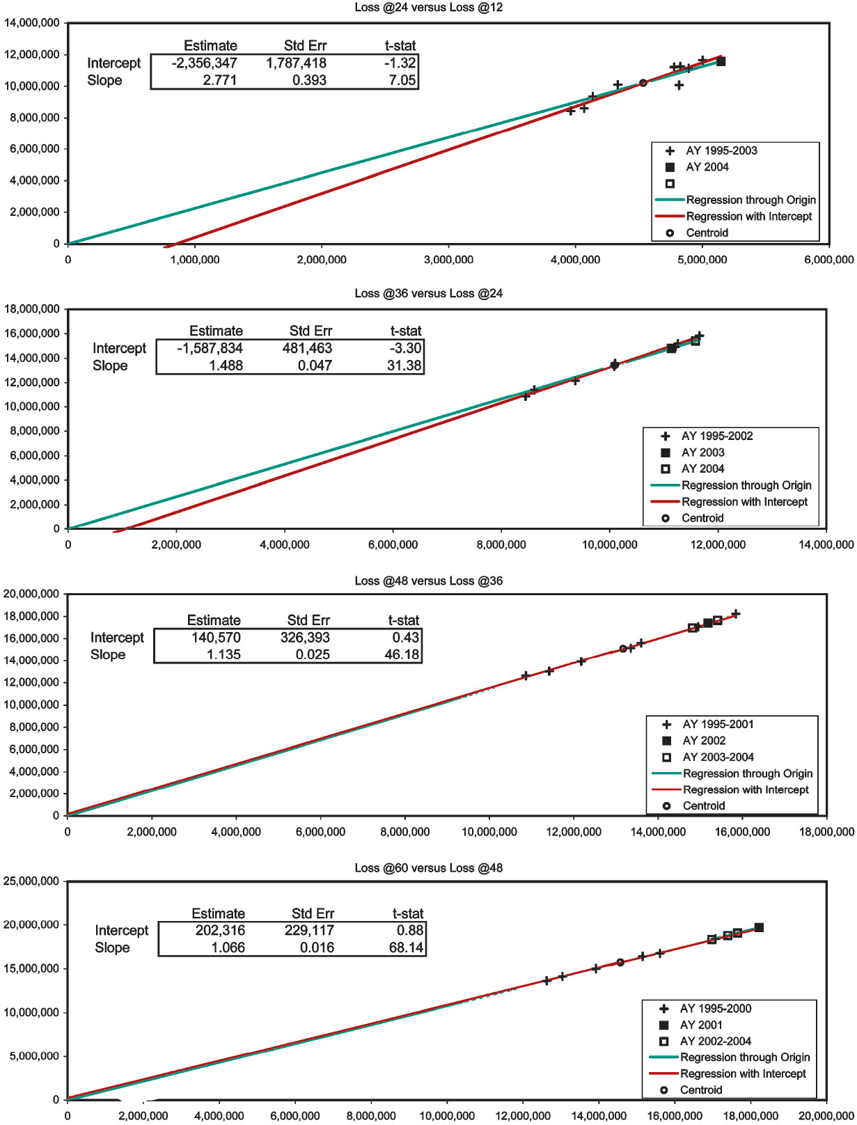
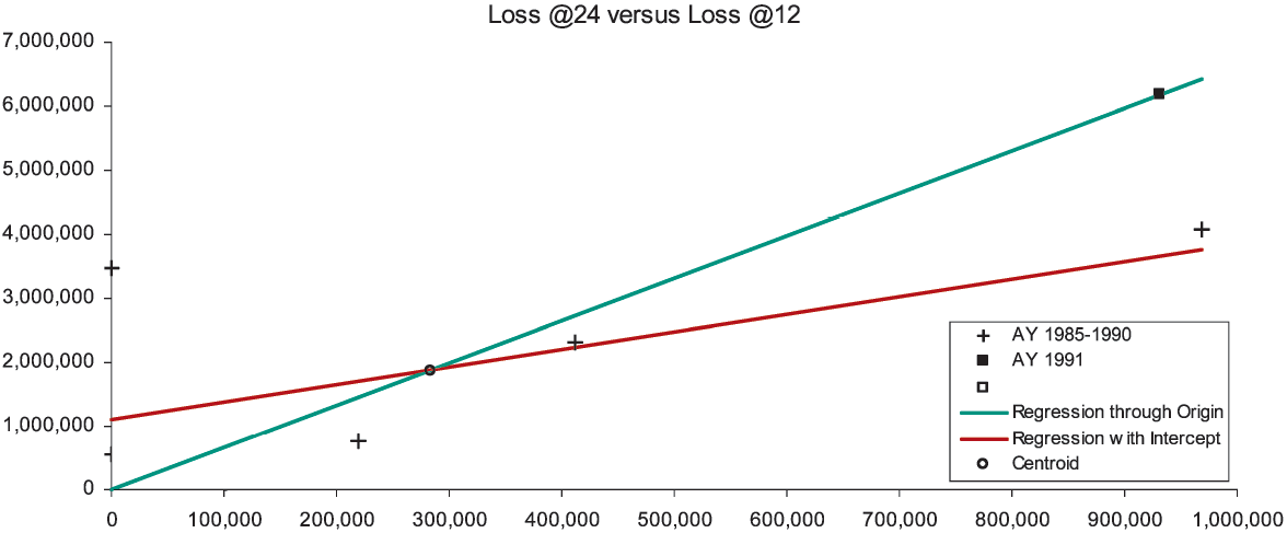
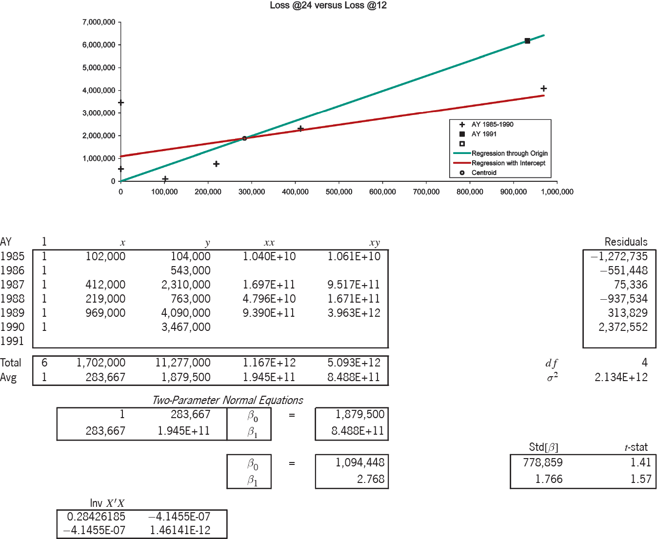
There are six observations of loss development from 12 to 24 months, which in Figure 1A are marked with the “+” symbol. The x-axis measures the loss at 12 months, the y-axis the loss at 24 months. We would like the observed points to lie close to a one-dimensional curve, viz., y ≈ ƒ(x). Then it would be a simple matter to develop AY (accident year) 1991 to 24 months as ƒ(932,000). For several reasons, but especially due to the scarcity of observations, we will consider only functions linear in x, i.e., y ≈ β₀ + β₁x. With a random error term, we make the formula exact, and arrive at a so-called “regression” model y = β₀ + β₁x + e. The expression “regression model” is unfortunate; a better name is “linear statistical model.” Appendix B details the theory of the linear statistical model.

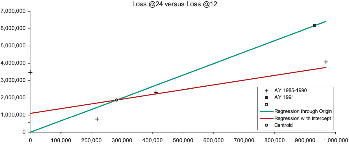
That the observations in Figure 1A do not line up well means that if the relation between E[y] and x is linear, it is obscured by an error term of significant variance. Nevertheless, the general line with intercept β₀ = $1,094,448 and slope β₁ = 2.768 (the red-colored line) must fit the observations better than the line constrained to pass through the origin (the green-colored line). This constrained line, with intercept zero and slope γ = 6.626 is the “regression-model” equivalent of the chain-ladder method. Appendix C specifies the variance assumptions of the two models (viz., the two-parameter is homoskedastic, the one-parameter is heteroskedastic), and proves that both lines must intersect at the centroid of the observations, i.e., at the average point (x, y). For all loss triangle applications the centroid will lie in the first quadrant of the Cartesian plane. Because the intercept of the general line is positive and the centroid lies in the first quadrant, to the left of the centroid the constrained line is below the general, and to the right of the centroid it is above.

Now our diagnosis rests on the following assumption: The general line is preferable to the constrained line. Our rationale is simple: For the purposes of diagnosing CL bias we have limited ourselves to linear functions, and the constrained line is a special case of the general. With the CL method we are, in effect, projecting along the constrained (green-colored) line, whereas we would be better off using the general (red-colored) line. So we develop AY 1991 as $932,000 × 6.626 = $6,175,184, which point on the constrained line is marked with the “◼” symbol. The point directly underneath on the general line would have a height of $3.7 million. On the basis of our assumptions, the CL method has considerably overpredicted.

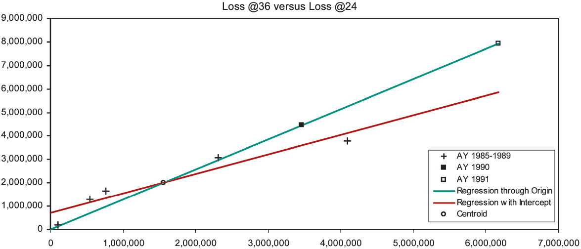
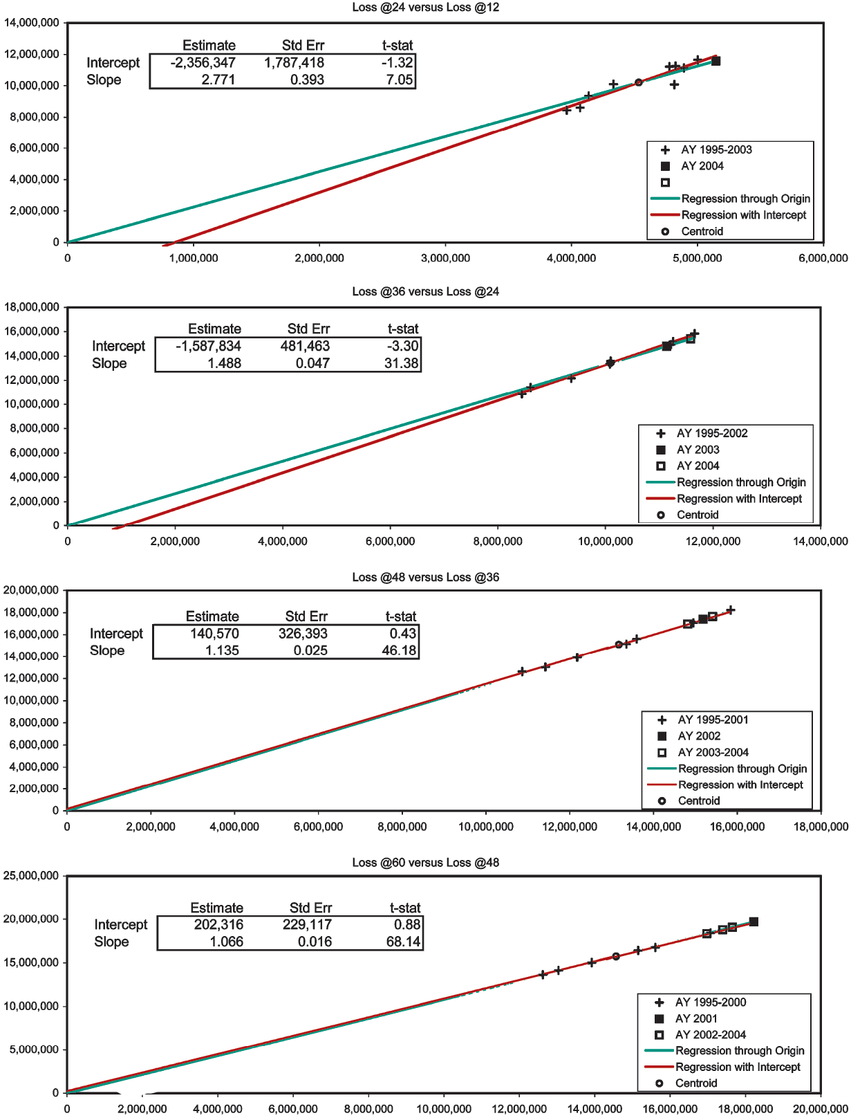
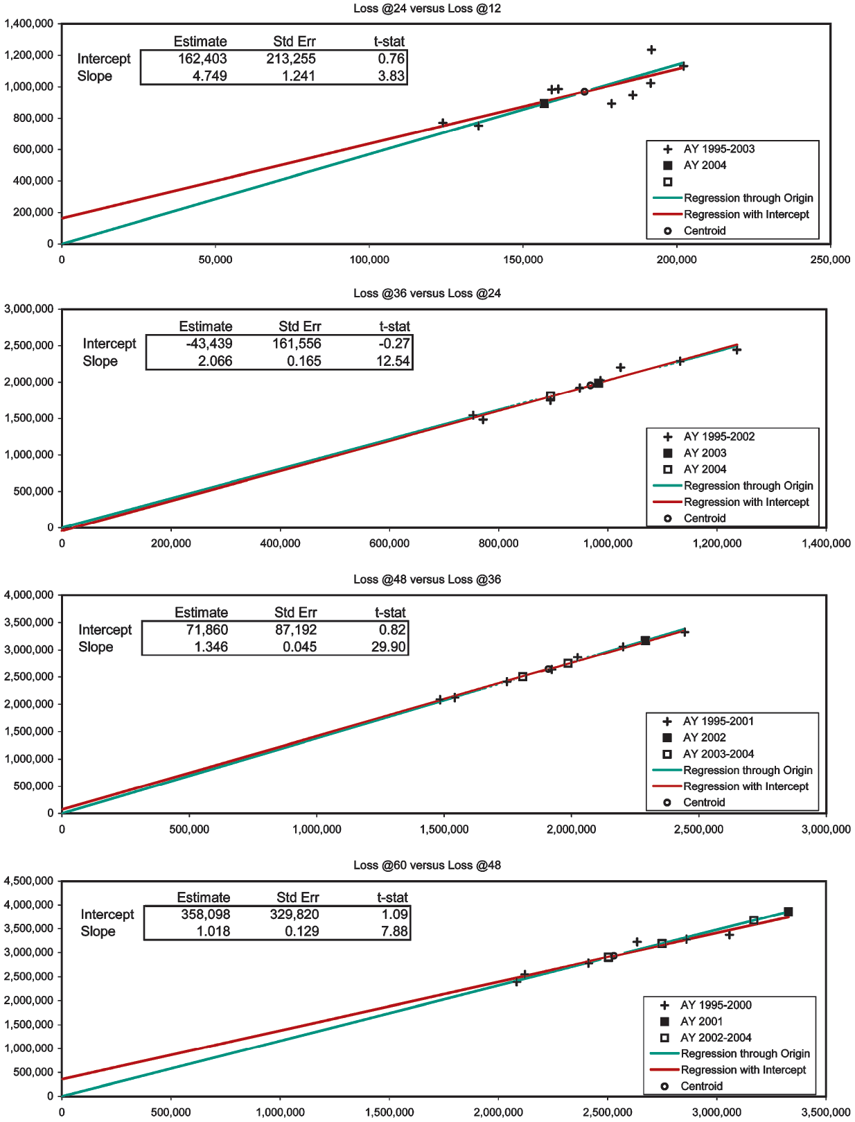
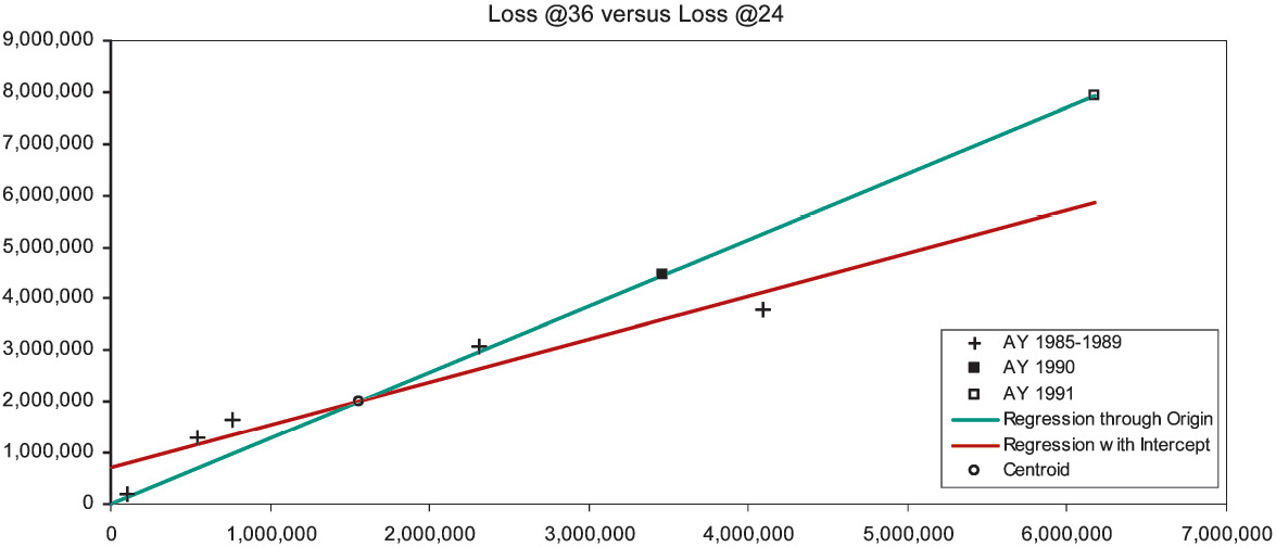
To diagnose the next link of the chain, the development from 24 to 36 months, we rely on Figure 1B. Now we are limited to five observations, which the figure shows as “+” signs. The general and the constrained lines are fitted, and their intersection is marked as the centroid. Again we find the intercept of the general line to be positive. Hence, according to our assumption, projections from x values to the left of the centroid will be too small, and projections to the right will be too large. AY 1990 at 24 months lies moderately to the right of the centroid and is moderately overpredicted. AY 1991 at 24 months, now marked with the “□” symbol, lies extremely to the right of the centroid and is much more overpredicted. In fact, the CL method has compounded the overprediction of AY 1991, since it first overpredicted its development from 12 to 24 months.

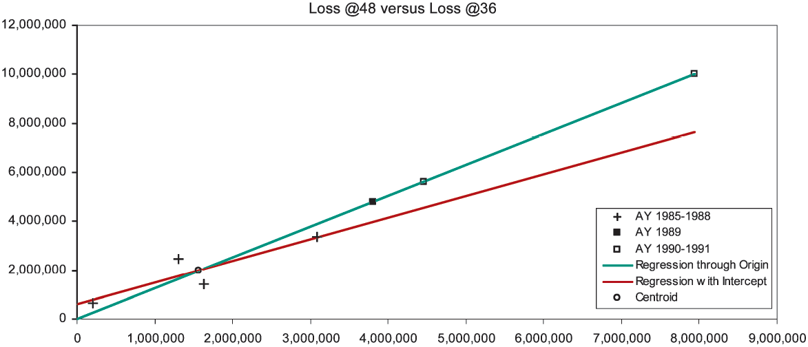
We repeat the diagnosis for the development from 36 to 48 months in Figure 1C. Although confidence in our lines is lessening, we still find the intercept to be positive; and all predictions are from x values to the right of the centroid. Therefore, we diagnose AY 1989 to be simply overpredicted, and AY 1990–1991 to be multiply overpredicted.

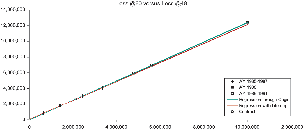
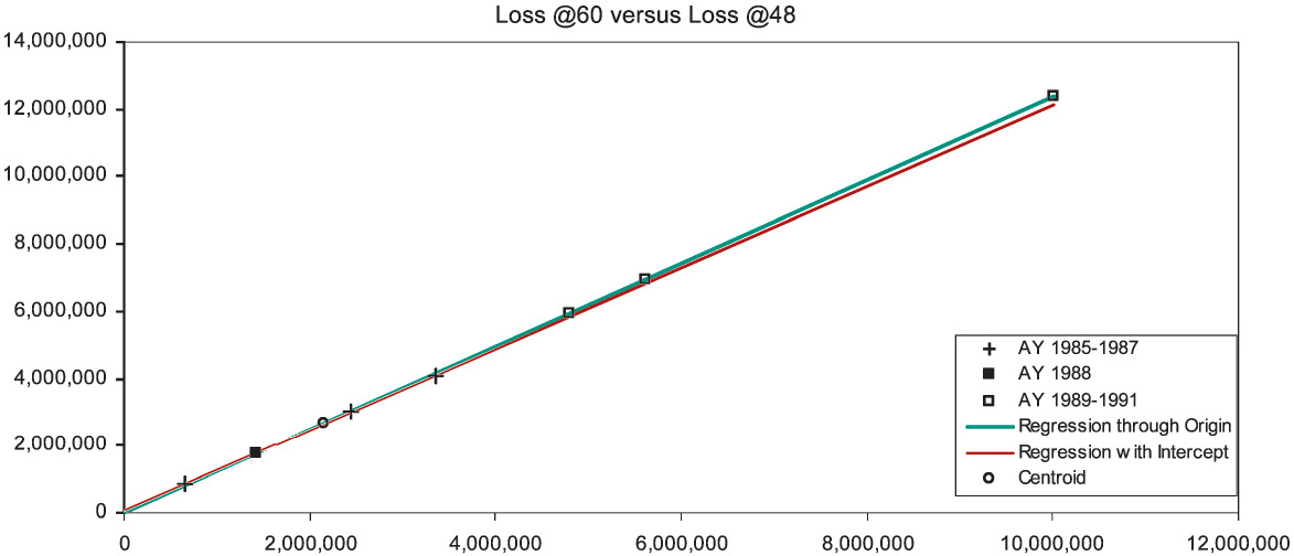
Finally, Figure 1D shows development from 48 to 60 months. At this stage the lines are nearly coincident; the CL method is trustworthy. Our final diagnosis rests on Table 2. AY 1988 at 60 months is fairly estimated as $1.76 million. The later accident years have been overestimated at 60 months, the overestimation compounding as the years advance. AY 1991 is overestimated to an uncharacteristically large 96% loss ratio.

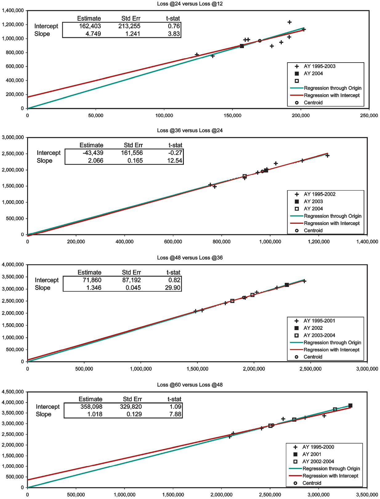
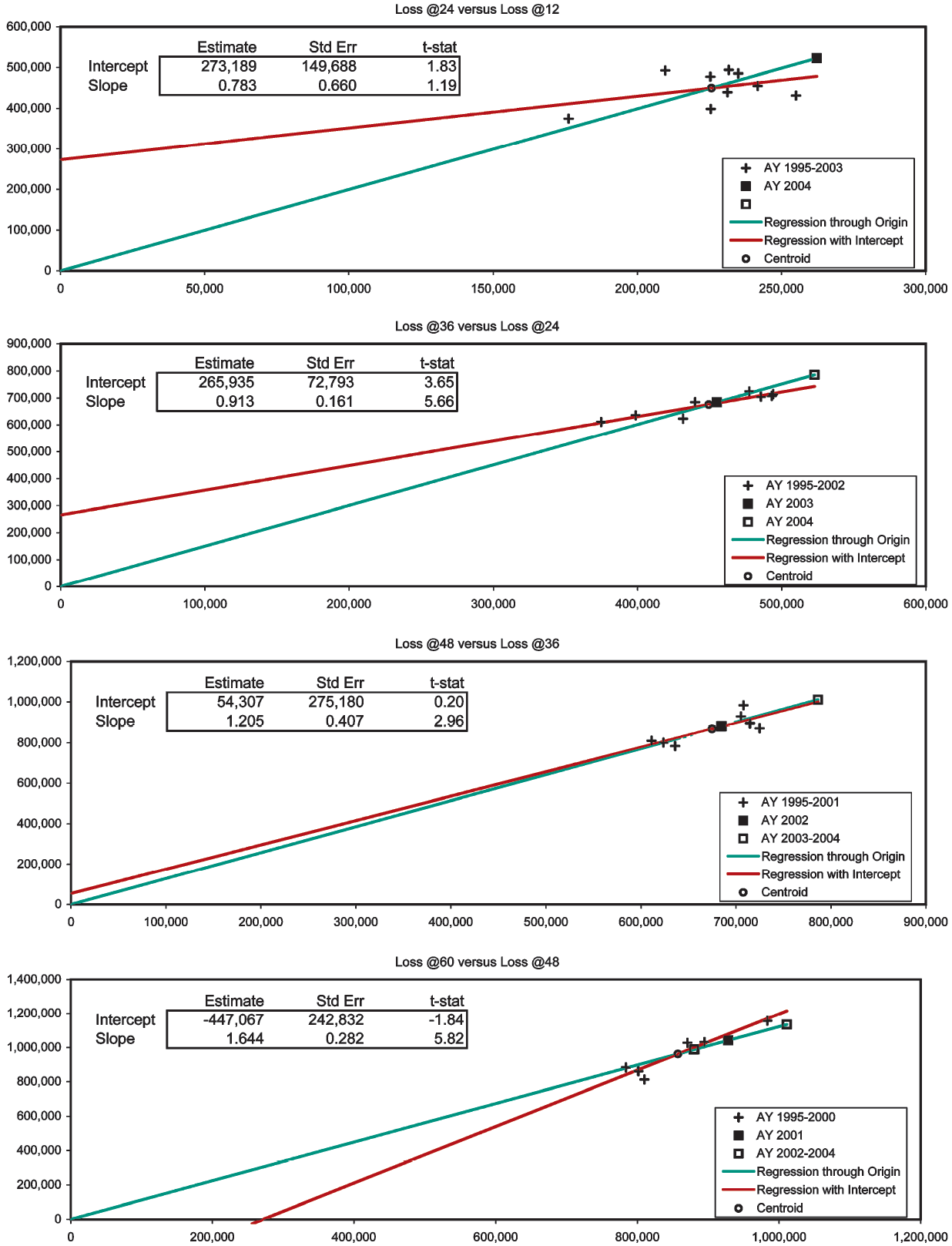
In Exhibits 2–4 we apply the diagnostic to consolidated Schedule-P triangles (Best’s Aggregates and Averages, Property/Casualty 2005, 199–213). These exhibits are more quantitative than Figures 1A–1D in that they contain the estimates, standard errors, and t statistics of the intercept and slope of the general lines.^[11] Since the t statistic equals the estimate divided by the standard error, the estimate is “t-stat” standard errors away from zero. If the error terms of the regression model are normally distributed, the t-stat will be t-distributed with n − 2 degrees of freedom, and a probabilistic significance can be assigned to it. Never assuming normally distributed error terms, we will simply abide by such qualitative standards as when the absolute value of the t statistic is greater than one the difference of the estimate from zero is fairly significant, when greater than two quite significant, and when greater than three very significant.

The first two development stages of the paid Workers’ Compensation triangle (Exhibit 2) show significant negative intercepts. Nevertheless, the CL-predictions are always close to their respective centroids. Development to 60 months is unexceptional. The paid Medical Malpractice triangle (Exhibit 3) displays mildly positive intercepts in the first and fourth development stages. We suspect AY 2001 to be slightly overpredicted. Exhibit 4 is the most interesting. To obtain this case-incurred triangle for Products Liability Occurrence we had to subtract the bulk + IBNR reserves (Schedule P, Part 4) from the incurred triangle (Schedule P, Part 2). The first two development stages have large positive intercepts, and the fourth has a large negative one. AY 2004 at 36 months has been twice overpredicted. Everything else stays close to the centroids, except for one underprediction from 48 to 60 months. This underprediction pertains to AY 2004, so at 60 months this AY has been twice overpredicted and once underpredicted, overall apparently netting a slight overprediction.

At each link or development stage, chain-ladder bias depends on the intercept of the general line. If it is positive, projections from less-than-average x values (to the left of the centroid) will underestimate, projections from greater-than-average x values (to the right of the centroid) will overestimate. The relation is reversed in the case of a negative intercept: projections to the right of the centroid underestimate, those to the left overestimate. CL bias becomes more serious as the intercept moves more significantly away from zero. The method is unbiased, if the regression lines coincide.

From this we venture to explain the anecdotes that the chain-ladder method overpredicts. First, in our experience with loss triangles, we have found significant positive intercepts more often than significant negative ones. Not having kept records, we cannot cite the proportions (significantly positive, significantly negative, not significantly different from zero). Certainly we do encounter intercepts significantly less than zero; here we found them in Exhibits 2 and 4. Nevertheless, not only are positive slopes more frequent than negative; they tend to be more statistically significant, as well.

Because the centroids are in the first quadrant, we can state the first empirical finding: Based on the preponderance of positive intercepts, more often than not the CL method will overpredict, or overdevelop, losses that are greater than average at any given maturity, i.e., losses to the right of the centroid. And second, as with the rest of the economy, it is normal for the insurance business to grow. In this condition exposures increase, and one expects the amounts down any column of a loss triangle to increase. Hence, the CL method commonly projects losses that lie to the right of the centroid. The combination of positive intercepts and business expansion makes for overprediction. The CL method would actually underpredict with the combination of positive intercepts and business contraction. The reverse would hold, if the intercepts were negative. In a triangle of mixed intercepts (i.e., some positive and some negative) conflicting forces would be at work; probably, however, forces at the earlier links would prevail at the overall level.

This explanation discredits appeals to “skewness,” i.e., to arguments that the upside of overprediction is unlimited, whereas the downside is limited to zero. For, indeed, the CL method is on average unbiased over the empirical distribution of the observed ordered pairs, and over any bivariate distribution that might be fitted to their moments. The observed (x,y) variables that average to the centroid may each have positive skewness. But the smaller number of large biases to the right of the centroid is offset by the larger number of small biases to the left. Of importance is the relation of the two lines over the domain of the x values that need to be developed.

4. Chain-ladder bias and the regression intercept

One might be tempted from the previous section to “fix” the chain-ladder method by projecting from the general line. At this point we are still within the framework of deterministic methods, i.e., methods that yield point estimates and provide no information about higher moments or probability distributions. Since the 1990s actuaries have advanced from methods to models in order to obtain probabilistic information. And within the modeling framework, this “fix” is tantamount to a movement from the Mack (Mack 1994, 107) model, E[y | x = x] = γx, to the Murphy (Murphy 1994, 187) model, y = β₀ + β₁x + e or E[y | x = x] = β₀ + β₁x (both models expressed in our notation).

But habits and paradigms are hard to identify, and hence to change. This can dispose one to read a model into, rather than out of, the data. Some have not pondered whether their models are truly reasonable and whether they really fit the data. As for a lack of fit, Barnett and Zehnwirth (Barnett and Zehnwirth 2000, 250) faults the Mack model: “It turns out that the assumption that, conditional on x(i), the “average” value of y(i) is bx(i), is rarely true for real loss development arrays.” And apart from the question of fitness, the Murphy-like addition of an intercept makes for an unreasonable model. For consider the general model of Figure 1A, whose parameters are estimated in Exhibit 5. The model for the six observations is y = $1,094,448 + 2.768x + e, where the standard deviation of the error term is \(\sqrt{2.134 \mathrm{E}+12}\) = $1,460,829. Above all, a model should be reasonable, and we fail to understand why the loss at 24 months should start from a base amount of $1,094,448. Accordingly, Gregory Alff (Alff 1984, 89) has written, “A constant does nothing to describe the underlying contributory causes of change in the dependent variable.” We can even imagine a condition in which an intercept must be rejected, namely, when one derives a negative intercept and projects from such a small x value that the projection itself is negative.

Furthermore, since the centroid is in the first quadrant, if the intercept is positive, the slope of the general line must be less than that of the constrained line. The flattened slope might well not differ significantly from unity.^[12] In such a situation it is not the ratio of the later loss to the earlier that is important, but the difference of the later loss from the earlier. If y − x is fairly constant, then it deserves modeling, not the quotient y/x.

Finally, the exposures of the six accident years range must vary widely. For the growth of premium from $4.3 to $12.0 million (and to $12.9 million in 1991) cannot be attributed to rate increases; exposure must be climbing over these years. If the exposure of one AY were twice that of another, perhaps its intercept should be twice.^[13] This reasonable thinking would lead the modeler to replace the constant with an exposure variable ξ: y = β₁x + β₂ξ + e. However, the earlier loss x and the exposure ξ usually compete, and one can be eliminated without much loss of explanatory power. The key to understanding this competition (“multicollinearity” in statistical parlance) is regression toward the mean, to which we now turn.

5. Regression toward the mean

The term “regression toward the mean” originated with Sir Francis Galton (1822–1911), who among other biological subjects applied it to the inheritance of height (Galton 1886). (See also [Wikipedia contributors, n.d.].) In this section we will simplify the excellent discussion in Chapter 12 “Regression and Correlation” of Bulmer (Bulmer 1979), and analogize from height inheritance to loss development.

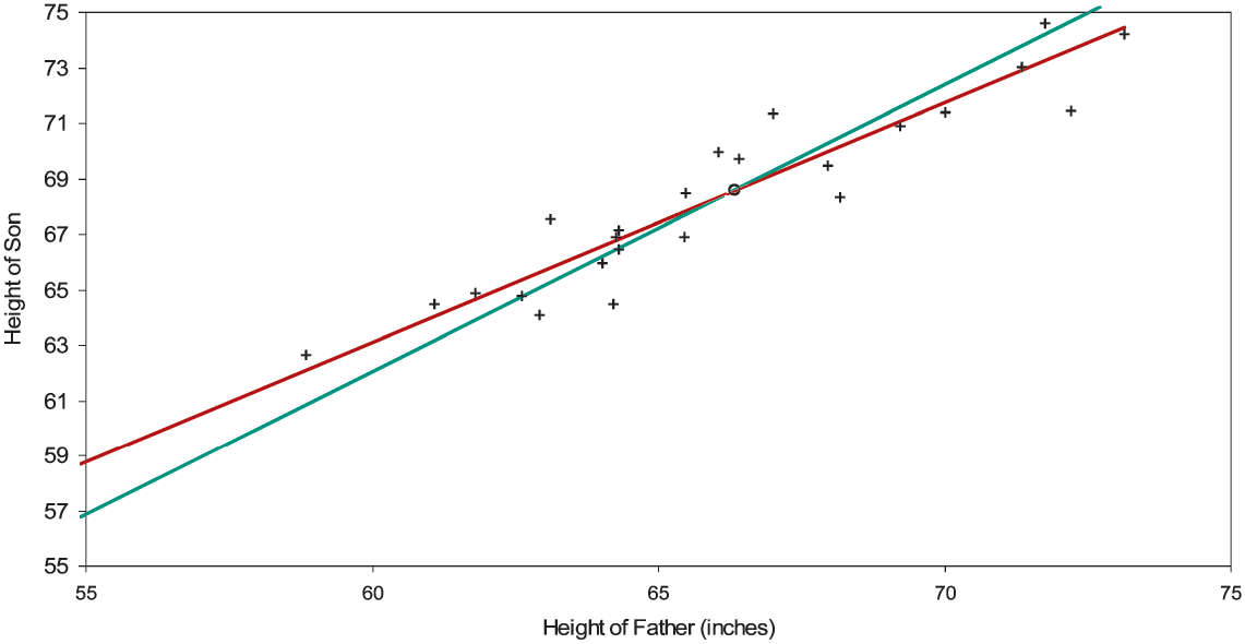
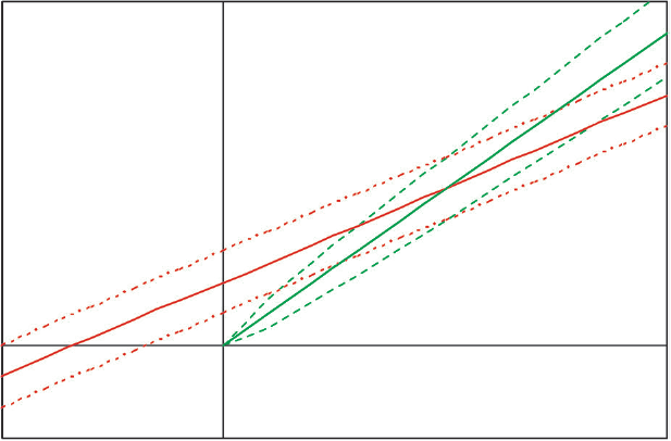
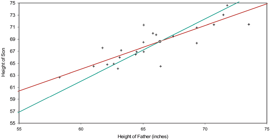
In Figure 2A are graphed 25 pairs of heights of fathers and sons, with their centroid and their best-fitting general and constrained lines. Although these points are simulated, they have all the verisimilitude of the data that Galton studied. To reveal up front our simulation mechanism would spoil the joy of repeating Galton’s discovery; we will discuss it shortly.

The centroid is (66.34, 68.60) inches. The intercept and the slope of the general line are 11.23 inches and 0.865; the slope of the constrained line is 1.034. We allowed for height “inflation” due to better care and nutrition: sons are on average about two inches taller than their fathers. One would like to regard a son’s height as proportional to his father’s; but the intercept of the general line with its standard error (11.23±4.32 inches) puts the intercept at a quite significant 2.60 standard errors away from zero. In other words, the data rebels against a line through the origin.

Data that regresses toward the mean is not to be confused with a process that reverts toward the mean. Figure 2A is a picture of regression toward the mean; the best-fitting line, though sharing the centroid of the constrained line, lies be-tween the constrained line and a horizontal line through the centroid. This implies that the intercept of the best line lies between zero and the ordinate of the centroid. A significant difference between the two lines means that somehow the data is defying proportionality.^[14]

Galton was convinced that the inheritance of height should be a proportion; there is no reason why nature should begin with 11.23 inches. So he drew the ingenious distinction between genetic height and empirical height. With a tape measure one records empirical height; but one’s empirical height is the sum of one’s genetic height and an environmental error term of mean zero. If one could peer into genetic height, one would see that that a son’s genetic height is proportional to his father’s. If one knew the genetic heights of fathers, the line that best fit the points of the fathers’ genetic heights and the sons’ empirical heights would pass through the origin. Hence, a best-fitting line regresses toward the mean because the independent variable actually used is a proxy (even though an unbiased proxy) for a better or truer variable.

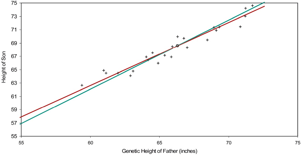
To a father 58.83 inches tall belongs the leftmost point in Figure 2A; to a father 73.13 inches tall the rightmost. Even though the mean of the environmental error term is zero, given that we are looking at a relatively short father, we infer that he is genetically taller than 58.83 inches, and that his error term is negative. So the short father is probably genetically less short than he is empirically. Similarly, the tall father is probably genetically less tall than he is empirically. And the more a father’s empirical height differs from the average (66.34 inches), the more his error term is expected to differ from zero. Lifting the veil from the fathers’ genetic heights (which we can do, since it’s a simulation), we have the result of Figure 2B. The centroid and the constrained line have not changed, but now the general line does not regress as much toward the mean. Its intercept and slope now are 5.96 inches and 0.945, which are not significantly different from the true values 0.00 inches and 1.030 (= 68/66). Switching the independent variable from empirical height to genetic contracts the x-axis toward the abscissa of the centroid and pivots counterclockwise the general line toward the constrained line.

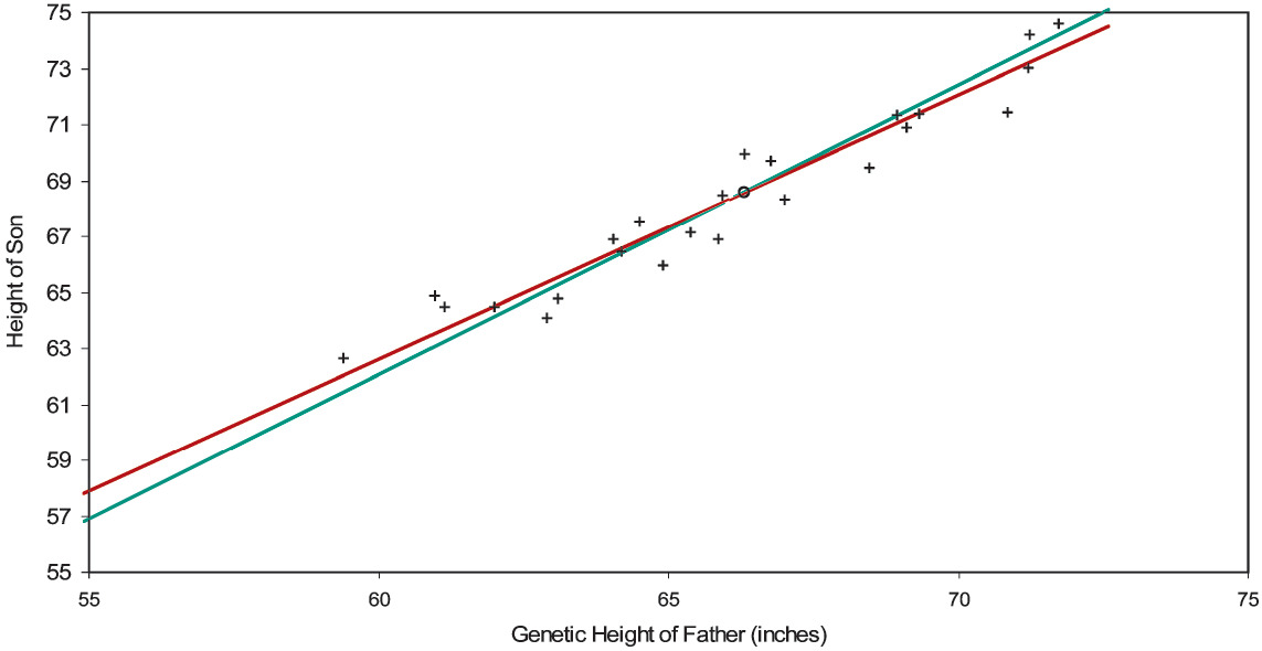
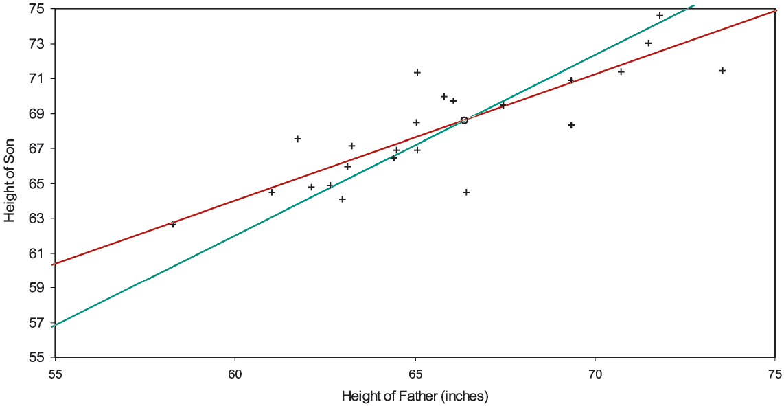
Moreover, the better a variable proxies for the true variable, the less the general line will regress toward the mean; the worse it proxies, the more the line regresses. As for our simulation mechanism, the genetic heights of the fathers were normally distributed as 66±4 inches. Then these values were multiplied by 68/66 to simulate the sons’ genetic heights. To both sets of heights were added normally distributed environmental terms whose mean and standard deviation were zero and one inch. So here the fathers’ genetic heights are relatively discernible; in actuarial parlance, the variance of the hypothetical means is (4 inches)² and the expectation of the process variance is (1 inch)². But in Figure 2C, starting with the same genetic heights and environmental errors, we’ve doubled the fathers’ environmental errors. This increases the regression toward the mean, the intercept and slope of the general line (with standard errors) now being 20.59±5.59 inches and 0.724±0.084. Environmental error weighs more heavily on genetic height; actuaries would say that the fathers’ heights are less credible.^[15] If the standard deviation of environmental error were many times the standard deviation of genetic height, a father’s empirical height would indicate little about his or his son’s genetic height, and the general line would be nearly flat—extreme regression toward the mean.^[16]

The analogy of Galton’s problem to loss development is straightforward. The father’s empirical height corresponds to the loss at the earlier stage of development, the son’s empirical height to the loss at the later stage. The common phenomenon of regression toward the mean indicates that the loss at the earlier stage is a proxy for something else. Without doubt, zero loss, as in Figure 1A, is a (misleading) proxy for a positive exposure.^[17] But this, we believe, is always the case. Even if a line that best fits the adjacent columns of a loss triangle passes tolerably close to the origin, it indicates only that the earlier loss is a tolerable proxy. In Figure 1D, losses at 48 months were a tolerable proxy for a variable truly predictive of losses at 60 months; in Figures 1A–C the earlier losses were not good proxies.

To take another example, Medical Malpractice is regarded as a volatile line of business; yet our diagnosis of its paid loss development to 60 months (Exhibit 3) showed that a chain-ladder projection would happen to be reliable. The regression toward the mean in the 12- to 24-month stage is rendered innocuous by the fact that the projection of AY 2004 is close to the centroid. Nevertheless, the earlier losses are still just proxies of something else. Sometimes proxies are good enough; but when they are not, we must expend the effort to recover the true variables.

In the previous section we mustered reasons why an intercept should make way for an exposure variable. Models that incorporate both earlier loss x and exposure ξ usually suffer from multicollinearity; the earlier loss usually has little of its own to say, merely mimicking exposure. So it will come as no surprise by now that the earlier loss is none other than a proxy of exposure.^[18] The loss triangle is a workhorse for the actuary, and will not be put out to pasture in the foreseeable future. But our diagnosis of triangles and our explanation of regression toward the mean together suggest that a column of exposures should be deemed an integral part of every loss triangle. The information really resides in the exposures—a fact obvious to ratemaking, but hardly less important to reserving.^[19]

6. Credibility and regression toward the mean

In the previous section we made passing reference to actuarial credibility theory. One actuary, Gary G. Venter (Venter 1987) related credibility theory to regression toward the mean; another, Eric Brosius (Brosius 1993) related it to loss development. But neither saw how significant regression toward the mean is to loss development, namely, that it indicates proxy variables. Furthermore, they both thought of credibility “forwards,” i.e., as applying to the dependent variable. Venter, for example, wrote, “Least squares credibility can be thought of as a least-squares regression estimate in which the dependent variable has not yet been observed.” (Venter 1987, 134). But the “backward” view to be presented here, applying credibility to the independent variable, will lend support to what we’ve just said about proxy variables.

Consider again the 12- to 24-month stage of the Brosius triangle, as modeled in Exhibit 5. The centroid of the six observations (x, y) equals ($283,667, $1,879,500). The slope of the constrained line is y/x = $1,879,500/$283,667 = 6.626 = γ, and we express this line in the functional form g(x) = γx = 6.626x. We express the general line in the form ƒ(x)= β₀ + β₁x = $1,094,448 + 2.768x. Since both lines intersect at the centroid, y = ƒ(x) = g(x). Therefore:

\[ \begin{aligned} f(x) & =0+f(x) \\ & =\bar{y}-f(\bar{x})+f(x) \\ & =\bar{y}-\beta_{0}-\beta_{1} \bar{x}+\beta_{0}+\beta_{1} x \\ & =\bar{y}+\beta_{1}(x-\bar{x}) \\ & =\bar{y}+\frac{\beta_{1}}{\gamma}(\gamma x-\gamma \bar{x}) \quad[\Rightarrow \gamma \neq 0] \\ & =\bar{y}+\frac{\beta_{1}}{\gamma}(g(x)-\bar{y}) \\ & =\left(1-\frac{\beta_{1}}{\gamma}\right) \bar{y}+\left(\frac{\beta_{1}}{\gamma}\right) g(x) \\ & =(1-Z) \bar{y}+Z g(x). \end{aligned} \]

The general line can be interpreted as a credibility-weighted average of the constrained line and the centroidal horizon. The credibility given to the chain-ladder projection, i.e., to g(x) = γx, is Z = (β₁/γ) = (β₁x/y), which in this case is 41.8%. The credibility of the CL projection is the ratio of the slopes, namely that of the general line to that of the constrained.^[20] The complement of the credibility applies to the “prior hypothesis” y.

Credibility-weighting the CL projection y = g(x) with y is what we call the “forward” view of credibility; credibility is applied to the dependent variable y. Even more interesting, and revealing of the proxy status of earlier losses, is what we will call the “backward” view of credibility. The backward view is like the switching in the previous section of the independent variable x, an attempt to peer behind the proxy into the true variable. We remarked that contracting the x-axis toward the abscissa of the centroid, pivots the general line counterclockwise into coincidence with the constrained line.

Credibility-weight each observed independent variable x with the average value, i.e., with the abscissa of the centroid x, to form the “contract-ed” variable w = (1 − Z)x + Zx. This does not disturb the centroid, because w = x. Because g is linear and invariant to Z, for any credibility Z:

\[ \begin{aligned} (1-Z) \bar{y}+Z g(x) & =(1-Z) g(\bar{x})+Z g(x) \\ & =g((1-Z) \bar{x}+Z x) \\ & =g(w). \end{aligned} \]

Consequently, credibility-weighting the CL-fitted dependent variables with y is equivalent to CL-fitting the credibility-weighted independent variables with x; in other words, credibility-weighting and CL-fitting (i.e., regressing through the origin) are commutative at any credibility.

But consider the regression of y against w according to the general line y = γ₀ + γ₁w. Using the formula of Appendix C and removing constants from the covariances, we derive:

\[ \begin{aligned} \gamma_{1} & =\frac{\operatorname{Cov}[w, y]}{\operatorname{Cov}[w, w]}=\frac{\operatorname{Cov}[(1-Z) \bar{x}+Z x, y]}{\operatorname{Cov}[(1-Z) \bar{x}+Z x,(1-Z) \bar{x}+Z x]} \\ & =\frac{\operatorname{Cov}[Z x, y]}{\operatorname{Cov}[Z x, Z x]}=\frac{1}{Z} \frac{\operatorname{Cov}[x, y]}{\operatorname{Cov}[x, x]} \\ & =\frac{1}{Z} \beta_{1} . \end{aligned} \]

Here β₁ is the slope estimator of the general line modeled on the uncontracted (or fully credible) independent variables. Desiring to unwind the regression toward the mean, we choose Z such that γ₀ = 0, or equivalently, γ₁ = y/w = y/x. Hence,

\[ Z=\frac{1}{\left(\frac{1}{Z}\right)}=\frac{\beta_{1}}{\left(\frac{1}{Z} \beta_{1}\right)}=\frac{\beta_{1}}{\gamma_{1}}=\frac{\beta_{1}}{\left(\frac{\bar{y}}{\bar{x}}\right)}=\frac{\beta_{1} \bar{x}}{\bar{y}}, \]

which is the credibility that we derived in the forward view. Though equivalent mathematically, the forward and backward views differ as to interpretation. Whereas the forward view faults the model while passing the data, the backward view faults the data while passing the model. Or, whereas the forward view shores up the outputs of the model, the backward view shores up the inputs. Recognizing this alternative viewpoint should open actuaries to consider earlier losses as exposure proxies. Just as tall fathers are genetically tall, but probably not quite as tall genetically as empirically, so too large losses conceal large relative exposures, but probably not quite as large relatively to the actual losses. Correspondingly, just as short fathers are genetically short, but probably not quite as short genetically as empirically, so too small losses conceal small relative exposures, but probably not quite as small relatively to the actual losses. Progress depends on piercing the veil.^[21]

7. Standard models of loss development

The standard models of loss development are all of the same form:

\[ \begin{aligned} \mathbf{y} & =(X) \beta+\mathbf{e}, \quad \operatorname{Var}[\mathbf{e}]=\sigma^{2} \Phi, \\ \mathbf{y}_{i j} & =\left(a_{i j} \xi_{i}\right) \beta_{j}+\mathbf{e}_{i j}, \quad \operatorname{Var}\left[e_{i j}\right]=\sigma^{2} \phi_{i j} . \end{aligned} \]

The dependent variable \(\mathbf{y}_{i j}\) is the incremental loss of the ith exposure period at the jth stage of development, i.e., the ijth cell of the loss rectangle.

As an example, Schedule P exhibits, apart from the “Prior” line, have 10 accident years (rows) and 10 development years (columns), which make for 10 × 10 = 100 cells. If the experience is complete, 55 cells are observed (when i + j ≤ 11) and 45 require prediction (i + j > 11). The vector y is then the 100 cells unraveled as a (100 × 1) column vector. The design matrix X has 100 rows; the number of its columns, which equals the number of parameters in β, depends on the model. The error term e, like y, is (100 × 1). The model requires the variance of e, a (100 × 100) matrix of the covariances of the elements of e.

Variance considerations lead us to incremental formulations. Because variance structures are on the order of n², it is desirable to keep them simple. The variances of these standard models are zero off the diagonal, but not necessarily constant (viz., unity) on the diagonal. In terms of the indices of the cells of the original rectangle:

\[ \operatorname{Cov}\left[\mathbf{e}_{\mathrm{ij}}, \mathbf{e}_{\mathrm{kl}}\right]=\sigma^{2}\left\{\begin{array}{ll} \phi_{i j} & \text { if } i=k \quad \text { and } \quad j=l \\ 0 & \text { otherwise } \end{array} .\right. \]

If all the ϕ_ij are equal, the variance structure is “homoskedastic”; otherwise it is “heteroskedastic.” Homoskedasticity is the sparsest variance structure, on the order of n⁰, or 1. Heteroskedasticity is a less sparse variance structure on the order of n; but it too asserts that no two cells of the rectangle covary. Non-covarying incremental losses within an exposure period imply covarying cumulative losses. For example, the covariance of cumulative losses at 48 months with those at 24 months in terms of 12-month incremental error terms is:

\[ \begin{array}{l} \operatorname{Cov}\left[\mathbf{e}_{12}+\mathbf{e}_{24}+\mathbf{e}_{36}+\mathbf{e}_{48}, \mathbf{e}_{12}+\mathbf{e}_{24}\right] \\ = \operatorname{Cov}\left[\mathbf{e}_{12}+\mathbf{e}_{24}, \mathbf{e}_{12}+\mathbf{e}_{24}\right] \\ +\operatorname{Cov}\left[\mathbf{e}_{36}+\mathbf{e}_{48}, \mathbf{e}_{12}+\mathbf{e}_{24}\right] \\ = \operatorname{Cov}\left[\mathbf{e}_{12}+\mathbf{e}_{24}, \mathbf{e}_{12}+\mathbf{e}_{24}\right]+0 \\ = \operatorname{Var}\left[\mathbf{e}_{12}+\mathbf{e}_{24}\right] . \end{array} \]

The covariance of two intraperiod cumulative losses equals the variance of the earlier cumulative loss. Devising a variance for incremental losses whose cumulative variance is zero off the diagonal is no more than a mathematical challenge; it is quite unrealistic. To avail ourselves of the simplicity of homo- and heteroskedastic models, we must model incremental losses, not cumulative. Incremental losses may indeed covary; but non-covariance will be our default assumption, an assumption that is testable.^[22]

The exposure of the ith exposure period is ξ_i, e.g., car-years, insured value, sales, or payroll. For the examples here, the a_ij factors will be unity; however, they allow the modeler to adjust, or to index, the exposures, much as Stanard (Stanard 1985, 128) did with Butsic’s inflation model. Perhaps the awareness that losses as proxies impound a simple accident-date inflation lent credence to the CL model. However, this benefit does not validate the use of a proxy when the true variable is available; nor is this a benefit in the more complicated situations. Actuaries have done their homework when they explicitly calculate and apply the adjustments—not only to the observed part of the triangle, but also and especially to the future part.

Considerable thought should be given to the variance relativities ϕ_ij. Most basically, they should be proportional to exposure. But they should be quadratic to the adjustment factors. Moreover, though our examples will ignore it, models should recognize that, per unit of exposure, some development stages are more volatile than others. If υ_j denotes the variance in stage j per unit of exposure, a reasonable formula is \(\phi_{i j}=a_{i j}^2 \xi_i v_j\). Fortunately, however, less depends on the variance structure than on the design; an inexact or even an improper variance structure detracts from the optimality (“bestness”—the “B” in BLUE^[23]) of the predictions, but not from the unbiasedness.

The equation \(\mathbf{y}_{i j}=\left(a_{i j} \xi_i\right) \beta_j+\mathbf{e}_{i j}\) specifies the additive model, the fourth of Stanard’s models. The parameter \(\beta_j\) represents the pure premium of the \(j\) th development stage. This would be the raw input to pricing a policy that covered the portion of incurred loss that emerges in the \(j\) th development stage. Perhaps not a marketable idea, it has theoretical value inasmuch as an ordinary policy could be synthesized from non-overlapping policies that cover all the time after inception.

The additive method is the most flexible of the standard methods; it presumes the least information about the loss development and hence has the greatest parameter variance. But if one knew what fraction of loss developed at each stage ( \(f_j\), which sum to unity),^[24] one could express \(\beta_j\) as \(f_j \beta\). The model would then be \(\mathbf{y}_{i j}= \left(a_{i j} \xi_i f_j\right) \beta+\mathbf{e}_{i j}\), and only one parameter, \(\beta\), the whole pure premium, would be estimated. This statistical model corresponds to the StanardBühlmann, or Cape-Cod, method, the third of Stanard’s methods.^[25] Presuming more knowledge of the loss development and consequently reducing the number of parameters to just one, this model’s parameter variance is less than that of the additive model.

If one knows not only the relativities of the loss-development pattern (i.e., the \(f_j\) factors), but also the magnitude of it (i.e., the whole pure premium \(\beta\)),^[26] one reduces to the Born-huetter-Ferguson model \(\mathbf{y}_{i j}=\left(a_{i j} \xi_i \beta_j\right) \cdot 1+\mathbf{e}_{i j}= \left(a_{i j} \xi_i f_j \beta\right) \cdot 1+\mathbf{e}_{i j}\), Stanard’s second method. This is a “high-information” model in which no parameters are estimated; hence, its predictions have no parameter variance. At most, one estimates the variance magnitude \(\sigma^2\), and derives the process variances \(\hat{\sigma}^2 \phi_{i j}\).

Table 3 shows the continuity of these three models in descending order of parameter complexity. The descending complexity appears in the leftward movement of variables from the parameter vector (β) to the design matrix (X). Finally, we will illustrate these models on the Brosius triangle.

8. Standard models of the Brosius triangle

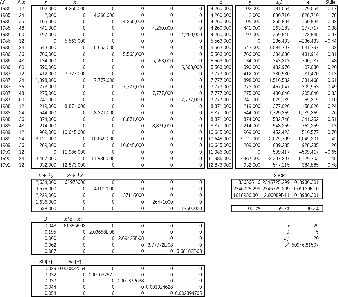
In Exhibit 6 we have readied the information for the three models. The Brosius triangle has seven accident years and five development stages for a total of 35 cells. The observations form an upper-left trapezoid of 25 cells; the predictions form a lower-right triangle of 10 cells. These two regions are the two boxes of the exhibit, whose rows are indexed by AY and Age. For lack of anything better, earned premium will serve as our exposure \(\xi_i\). Losses \(\mathbf{y}_{i j}\) are here incrementalized from the cumulative format of Exhibit 1. As mentioned in the previous section, all exposure and variance-relativity adjustments, \(a_{i j}\) and \(v_j\), are unity for the sake of simplicity. The next column contains the adjusted exposures \(a_{i j} \xi_i\), which form the design matrix of the additive model. The following column equals \(\phi_{i j}=a_{i j}^2 \xi_i v_j\), which we above claimed as a reasonable formula for variance relativity. These relativities will be used in all three models. The rightmost two columns contain the elements of the design matrices of the Stanard-Bühlmann and Bornhuetter-Ferguson models, as per the formulas of Table 3. However, the \(f_j\) factors and the overall “pure premium” (more accurately here, “loss ratio”) \(\beta\), were borrowed from the additive solution \(\boldsymbol{\beta}\) in Exhibit 7A. Therefore, the predictions from all three models must be the same; only the prediction-error variances will differ.

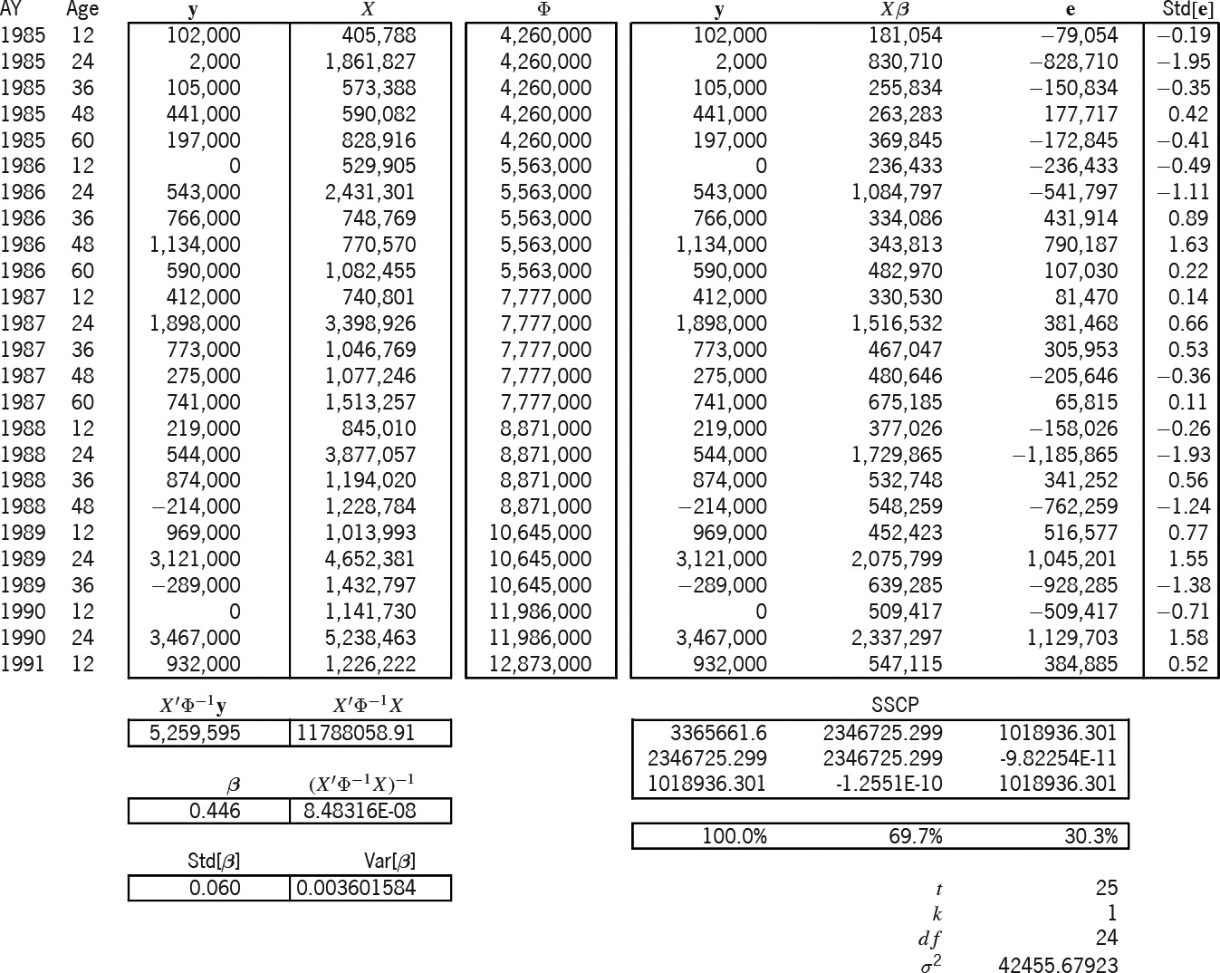
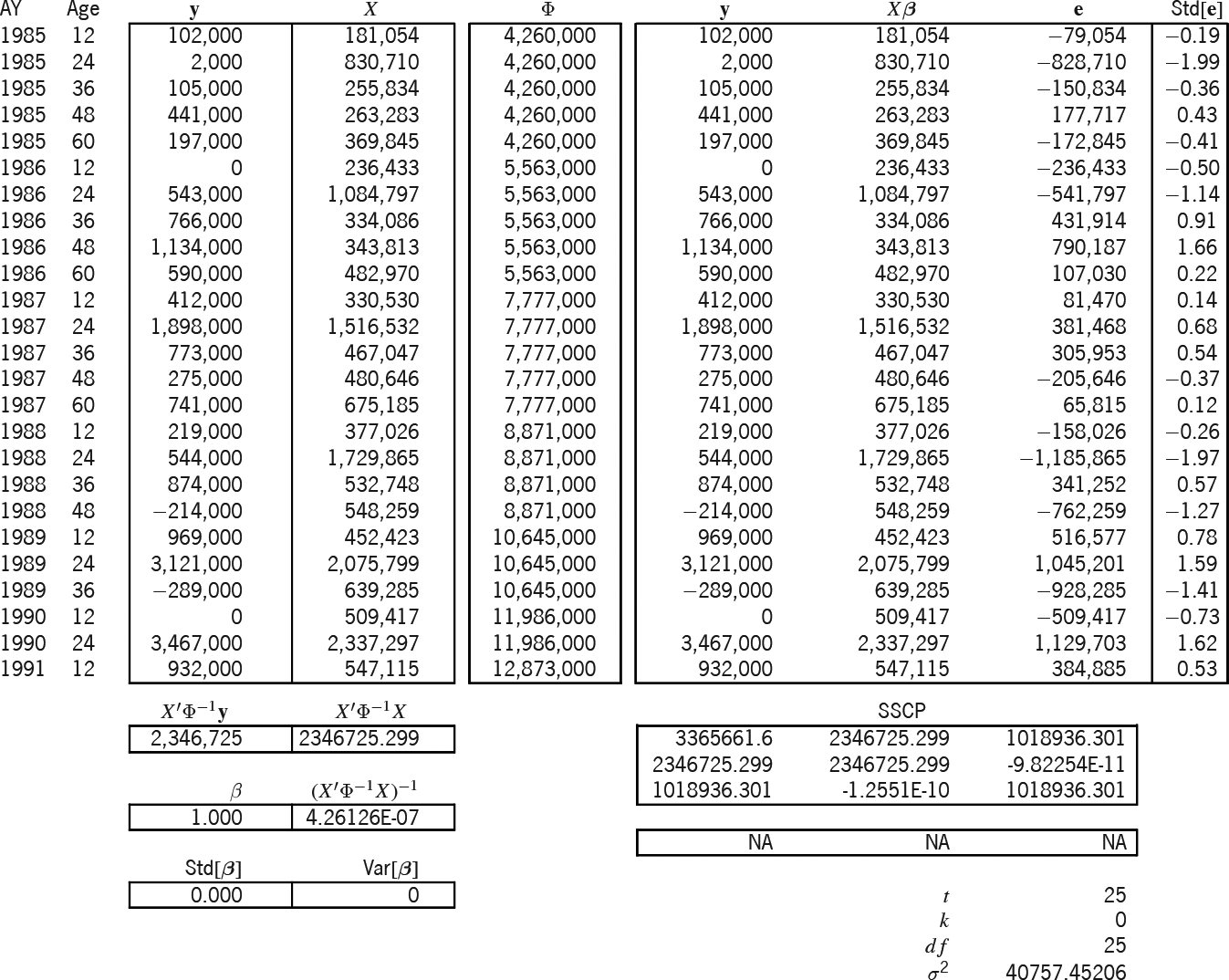
Exhibit 7A models the 25 observations (y) according to the additive design (X). Because the additive model has five parameters, the additive entries of Exhibit 6 must be slotted into the proper columns, as determined by the Age index (i.e., [0–]12 months slots into the first column, [12–]24 months into the second, etc.). The “Φ” column is the main diagonal of a (25 × 25) matrix of variance relativities; but in Excel it is just easier to treat it as a column and to multiply element-wise instead of matrix-wise.

Below these matrices are intermediate calculations that lead to the estimator \(\hat{\boldsymbol{\beta}}=\left(X^{\prime} \Phi^{-1} X\right)^{-1} \cdot X^{\prime} \Phi^{-1} \mathbf{y}\). This is the estimator of Appendix B, but it has been modified for heteroskedasticity (i.e., \(\Phi \neq I\) ). Appendix C shows a particular instance of this modification. The formula for " \(\operatorname{Var}[\boldsymbol{\beta}]\) " is \(\sigma^2\left(X^{\prime} \Phi^{-1} X\right)^{-1}\), the square root of whose diagonal is " \(\operatorname{Std}[\boldsymbol{\beta}]\)." Thus we estimate probabilistically \(\beta_{12}\) as \(0.043 \pm 0.029\).

Let \(M\) be the \((25 \times 3)\) matrix whose columns are \(\mathbf{y}, X \boldsymbol{\beta}\), and \(\mathbf{e}\) (the observed, fitted, and residual values). The “sums-of-squares-and-crossproducts” (SSCP) matrix is \(M^{\prime} \Phi^{-1} M\). If a parameter is fit, the diagonal elements of this matrix satisfy the equation \(m_{11}=m_{22}+m_{33}\). A rhosquare statistic (without intercept) based on this equation allows us to say that this model explains \(69.7 \%\) of what was observed. Finally,

\[ \hat{\sigma}^{2}=\frac{m_{33}}{t-k}=\frac{(\mathbf{y}-X \hat{\boldsymbol{\beta}})^{\prime} \Phi^{-1}(\mathbf{y}-X \hat{\boldsymbol{\beta}})}{t-k} \]

is the estimator for the scale of the variances; it is just the formula of Appendix B adjusted for heteroskedasticity (Φ⁻¹). The formula for the standardized residuals, Std[e],^[27] is e/\(\sqrt{\sigma^{2} \Phi}\). Standardized results outside the range [−2,2] may indicate model deficiencies.

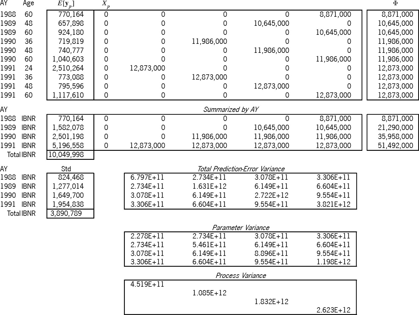
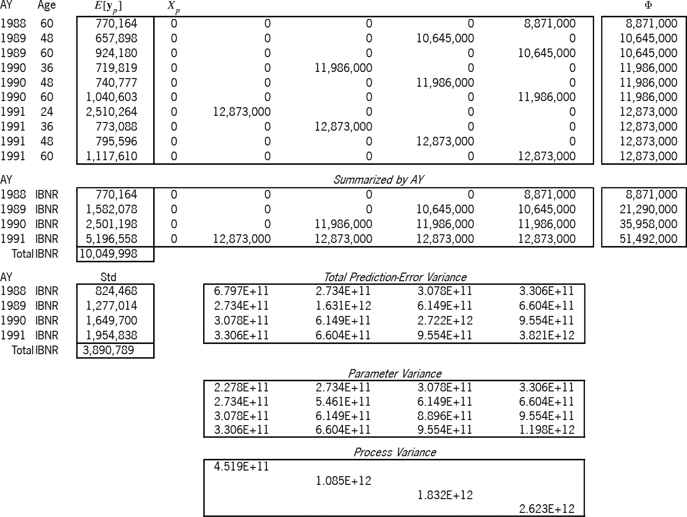
Exhibit 7B applies this solution to the prediction of the 10 cells of the lower-right triangle. The design of the prediction is the ( \(10 \times 5\) ) matrix \(X_p\). The expectation of the prediction is \(E\left[\mathbf{y}_p\right]=X_p \hat{\boldsymbol{\beta}}\). Again, the " \(\Phi\) " column is the main diagonal of a ( \(10 \times 10\) ) matrix of variance relativities. The formula for the prediction-error variance, i.e., for \(\operatorname{Var}\left[\mathbf{y}_p-E\left[\mathbf{y}_p\right]\right]\), is \(X_p \operatorname{Var}[\hat{\boldsymbol{\beta}}] X_p^{\prime}+ \sigma^2 \Phi\), whose two terms respectively are the parameter and the process variance. We summarized the \(X_p\) matrix by accident year, since the exhibit more easily accommodates ( \(4 \times 4\) ) matrices than ( \(10 \times 10\) ). All future “Age” values in the summarization are labeled “IBNR.”

A powerful feature of the linear statistical model is that the best linear unbiased estimator (BLUE) of a linear combination of a random vector is the linear combination of the BLUE of the vector, i.e., \(\operatorname{BLUE}[A \mathbf{y}]=A \operatorname{BLUE}[\mathbf{y}]\). So the formula \(X_p \operatorname{Var}[\hat{\boldsymbol{\beta}}] X_p^{\prime}+\sigma^2 \Phi\) holds true, whether \(X_p\) and \(\Phi\) are summarized or not. Both parts of the total prediction-error variance utilize the estimator \(\hat{\sigma}^2\). The square root of the diagonal of this variance matrix (the “Std” column) is the prediction-error standard deviation by accident year. Hence, this method probabilistically estimates AY 1991 IBNR as $5,196,558 \(\pm\) $ 1,954,838. The variance of the AY 1988-1991 total prediction-error variance; hence the total IBNR is $10,049,998±$3,890,789.

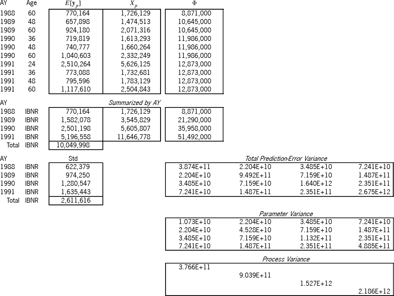
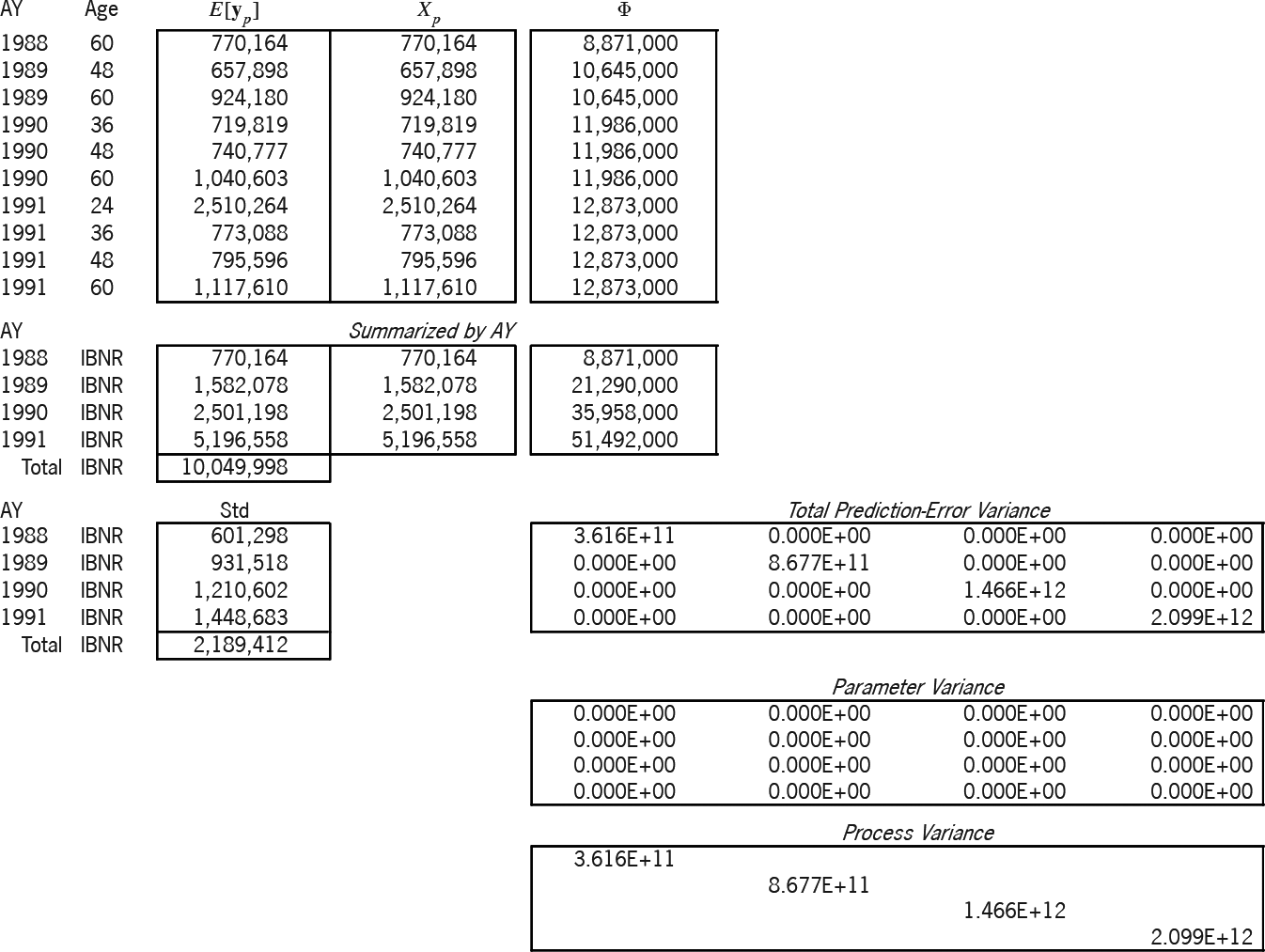
Exhibits 8A and 8B solve and predict according to the Stanard-Bühlmann model. This model has only one parameter; hence, the “SB” column of Exhibit 6 is the (25 × 1) design matrix X. The Bornhuetter-Ferguson (BF) model of Exhibits 9A and 9B seems to have one parameter; but in reality, it is set to unity, which is why the betas of Exhibit 9A are not in the bold font indicative of random variables, why the rho-square statistic is not applicable,^[28] and why the variance of the parameter is zero. Hence, the BF parameter variance in Exhibit 9B is zero.

Table 4 compares the accident-year IBNR results of the three models. As mentioned above, because the ƒ_j factors and the overall β were borrowed from the additive solution β, the models yield the same expected results. But the table illustrates the increasing prediction-error variance, primarily due to the progression of parameters from zero, to one, and then to five.^[29]

9. Conclusion

Is the chain-ladder method biased? In Section 2 we found the pioneering work of James Stanard suggestive of an answer, but not conclusive. In the next two sections we created a diagnostic tool and learned how the CL method behaves when regression lines refuse to pass through the origin. We discovered that regression toward the mean, coupled with business expansion, biases the CL method to overpredict. Next, in Section 5, Galton showed us that regression toward the mean is symptomatic of proxy variables. The following section reinforced this insight from the actuarial perspective of credibility. From all this we conclude that the chain-ladder method is biased. The bias most commonly takes the form of regression toward the mean, which indicates that earlier losses are serving as proxies for exposure—and the poorer the proxy, the more biased the method. The lesson to be learned from chain-ladder bias, or its meaning for us, is that loss-development models, in addition to being reasonable and empirically tested, should be free of proxy variables as much as possible. In Sections 7 and 8 we reformulated the Bornhuetter-Ferguson, Stanard-Bühlmann, and additive methods as a continuum of exposure-based loss-development models. It was because of this well-chosen base that Stanard found their performance superior to that of the chain-ladder method.