The Common Shock Model for Correlated Insurance Losses

1. Introduction

In the study of insurer enterprise risk management, “correlation” has been an important but elusive phenomenon. Those who have tried to model insurer risk assuming independence have almost always understated the variability that is observed in publicly available data. Most actuaries would agree that correlation is the major missing link in the realistic modeling of insurance losses.

This paper discusses an approach to the correlation problem in which losses from different lines of insurance are linked by a common variation (or shock) in the parameters of each line’s loss model. Here is an outline of what is to follow.

• A simple common shock model will graphically illustrate the effect of the magnitude of the shocks on correlation.

• The paper will describe some more general common shock models that involve common shocks to both the claim count and claim severity distributions. The paper will derive formulas for the correlation between lines of insurance in terms of the magnitude of the common shocks and the parameters of the underlying claim count and claim severity distributions.

• Finally, we will see how to estimate the magnitude of the common shocks. A feature of this estimation is that it uses the data from several insurers.

One should note that the common shock model is a kind of a “dependency” that causes correlation. It is possible for highly dependent random variables to be uncorrelated.

2. A simple common shock model

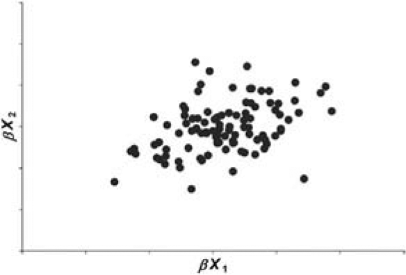
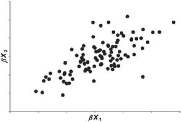
Let X₁ and X₂ be independent positive random variables. Also let β, which is independent of X₁ and X₂, be a positive random variable with mean 1 and variance b. If b > 0, the random variables βX₁ and βX₂ tend to be larger when β is large, and tend to be smaller when β is small. Hence the random variables βX₁ and βX₂ are correlated. Figures 1 through 4 illustrate this graphically for the case in which X₁ and X₂ follow a gamma distribution.

Figure 1.$X_1$ and $X_2$ are independently drawn random variables with a coefficient of variation (CV) equal to $0.1 . \beta$ is drawn from a distribution with $b=\operatorname{Var}[\beta]=0$. Thus $\rho=0.00$

Figure 2.$X_1$ and $X_2$ are independently drawn random variables with $C V=0.1 . \beta$ was drawn from a distribution with $b=\operatorname{Var}[\beta]=0.005$. Thus $\rho=0.33$

Figure 3.$X_1$ and $X_2$ are independently drawn random variables with $C V=0.1 . \beta$ was drawn from a distribution with $b=\operatorname{Var}[\beta]=0.020$. Thus $\rho=0.66$

Figure 4.$X_1$ and $X_2$ are independently drawn random variables with $C V=0.2$. $\beta$ was drawn from a distribution with $b=\operatorname{Var}[\beta]=0.020$. Thus $\rho=0.33$

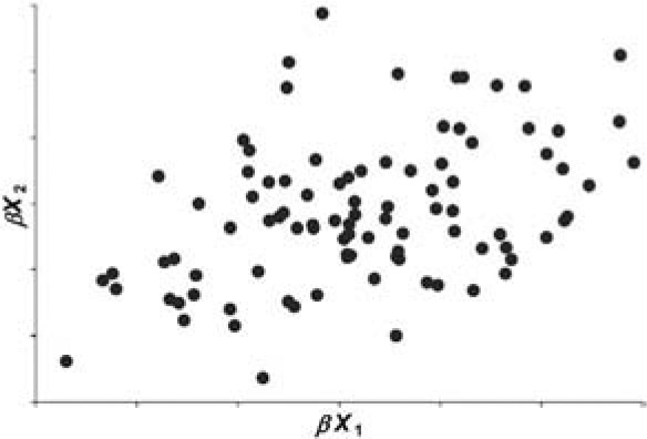
Let us refer to β as the “common shock” and refer to b as the magnitude of the common shock. Figures 1 through 4 illustrate graphically that the coefficient of correlation depends upon b and the volatility of the gamma distributed random variables X₁ and X₂.

We now turn to deriving formulas for the coefficient of correlation between the random variables βX₁ and βX₂. This derivation will be detailed. It is worth the reader’s time to master these details in order to appreciate much of what is to follow.

Let us begin with the derivation of two general equations from which to derive much of what follows. These equations calculate the global covariance (or variance) in terms of the covariances (or variances) that are given conditionally on a parameter θ.

$$\begin{aligned} \operatorname{Cov}[X, Y] & \\ = & \mathrm{E}[X \cdot Y]-\mathrm{E}[X] \cdot \mathrm{E}[Y] \\ = & \mathrm{E}_{\theta}[\mathrm{E}[X \cdot Y \mid \theta]]-\mathrm{E}_{\theta}[\mathrm{E}[X \mid \theta]] \cdot \mathrm{E}_{\theta}[\mathrm{E}[Y \mid \theta]] \\ = & \mathrm{E}_{\theta}[\mathrm{E}[X \cdot Y \mid \theta]]-\mathrm{E}_{\theta}[\mathrm{E}[X \mid \theta] \cdot \mathrm{E}[Y \mid \theta]] \\ & +\mathrm{E}_{\theta}[\mathrm{E}[X \mid \theta] \cdot \mathrm{E}[Y \mid \theta]] \\ & -\mathrm{E}_{\theta}[\mathrm{E}[X \mid \theta]] \cdot \mathrm{E}_{\theta}[\mathrm{E}[Y \mid \theta]] \\ = & \mathrm{E}_{\theta}[\operatorname{Cov}[X, Y \mid \theta]]+\operatorname{Cov}_{\theta}[\mathrm{E}[X \mid \theta], \mathrm{E}[Y \mid \theta]] . \end{aligned} \tag{2.1}$$

An important special case of this equation occurs when X = Y.

$$\operatorname{Var}[X]=\mathrm{E}_{\theta}[\operatorname{Var}[X \mid \theta]]+\operatorname{Var}_{\theta}[\mathrm{E}[X \mid \theta]] . \tag{2.2}$$

Now let us apply Equations (2.1) and (2.2) to the common shock model given at the beginning of this section.

$$\begin{aligned} \operatorname{Cov}\left[\beta X_{1}, \beta X_{2}\right]= & \mathrm{E}_{\beta}\left[\operatorname{Cov}\left[\beta X_{1}, \beta X_{2} \mid \beta\right]\right] \\ & +\operatorname{Cov}_{\beta}\left[\mathrm{E}\left[\beta X_{1} \mid \beta\right], \mathrm{E}\left[\beta X_{2} \mid \beta\right]\right] \\ = & \mathrm{E}_{\beta}\left[\beta^{2} \operatorname{Cov}\left[X_{1}, X_{2} \mid \beta\right]\right] \\ & +\operatorname{Cov}_{\beta}\left[\beta \mathrm{E}\left[X_{1}\right], \beta \mathrm{E}\left[X_{2}\right]\right] \\ = & \mathrm{E}_{\beta}\left[\beta^{2} \cdot 0\right]+\mathrm{E}\left[X_{1}\right] \cdot \mathrm{E}\left[X_{2}\right] \\ & \cdot \operatorname{Cov}_{\beta}[\beta, \beta] \\ = & \mathrm{E}\left[X_{1}\right] \cdot \mathrm{E}\left[X_{2}\right] \cdot b. \end{aligned} \tag{2.3}$$

$$\begin{aligned} \operatorname{Var}\left[\beta X_{1}\right] & =\mathrm{E}_{\beta}\left[\operatorname{Var}\left[\beta X_{1} \mid \beta\right]\right]+\operatorname{Var}_{\beta}\left[\mathrm{E}\left[\beta X_{1} \mid \beta\right]\right] \\ & =\mathrm{E}_{\beta}\left[\beta^{2} \cdot \operatorname{Var}\left[X_{1}\right]\right]+\operatorname{Var}_{\beta}\left[\beta \cdot \mathrm{E}\left[X_{1}\right]\right] \\ & =\operatorname{Var}\left[X_{1}\right] \cdot \mathrm{E}_{\beta}\left[\beta^{2}\right]+\mathrm{E}\left[X_{1}\right]^{2} \cdot \operatorname{Var}_{\beta}[\beta] \\ & =\operatorname{Var}\left[X_{1}\right] \cdot(1+b)+\mathrm{E}\left[X_{1}\right]^{2} \cdot b. \end{aligned} \tag{2.4}$$

Similarly:

$$\operatorname{Var}\left[\beta X_{2}\right]=\operatorname{Var}\left[X_{2}\right] \cdot(1+b)+\mathrm{E}\left[X_{2}\right]^{2} \cdot b . \tag{2.5}$$

The following equation defines the coefficient of correlation of two random variables, βX₁ and βX₂.

$$\rho\left[\beta X_{1}, \beta X_{2}\right]=\frac{\operatorname{Cov}\left[\beta X_{1}, \beta X_{2}\right]}{\sqrt{\left.\operatorname{Var}\left[\beta X_{1}\right] \cdot \operatorname{Var}\left[\beta X_{2}\right]\right]}}. \tag{2.6}$$

Combining Equations (2.3) through (2.5) with Equation (2.6) yields a simple expression for the correlation coefficient of βX₁ and βX₂ if we give X₁ and X₂ identical distributions with a common coefficient of variation, CV.

$$\rho\left[\beta X_{1}, \beta X_{2}\right]=\frac{b}{(C V)^{2} \cdot(1+b)+b} .\tag{2.7}$$

The coefficients of correlation given in Figures 1 through 4 were calculated using Equation (2.7).

At this point we can observe that the common shock model, as formulated above, implies that the coefficient of correlation depends not only on the magnitude of the shocks, but also on the volatility of the distributions that receive the effect of the random shocks.

3. The collective risk model

The collective risk model describes the distribution of total losses arising from a two-step process where: (1) the number of claims is random; and (2) for each claim, the claim severity is random. This section specifies a particular version of the collective risk model. The next section subjects both the claim count and claim severity distributions to common shocks across different lines of insurance and calculates the correlations implied by this model.

It will be helpful to think of the “common shocks” as either inflation or judicial trends that affect two or more lines of insurance simultaneously. The more severe shocks such as those caused by natural catastrophes are not the focus of this paper.

Let’s begin by considering a Poisson distribution with mean λ and variance λ for the claim count random variable N. Let χ be a random variable with mean 1 and variance c. The claim count distribution^[1] for this version of the collective risk model will be defined by the two-step process where (1) χ is selected at random; and (2) the claim count is selected at random from a Poisson distribution with mean χλ. The mean of this distribution is λ. Let’s refer to the parameter c as the contagion parameter.

Using Equation (2.2), one calculates the variance of N as:

$$\begin{aligned} \operatorname{Var}[N] & =\mathrm{E}_{\chi}[\operatorname{Var}[N \mid \chi]]+\operatorname{Var}_{\chi}[\mathrm{E}[N \mid \chi]] \\ & =\mathrm{E}_{\chi}[\chi \lambda]+\operatorname{Var}_{\chi}[\chi \lambda] \\ & =\lambda+c \cdot \lambda^{2}. \end{aligned} \tag{3.1}$$

Let $Z_i$ be a random variable for claim severity for the $i$ th claim. We will assume that each $Z_i$ is identically distributed with mean $\mu$ and variance $\sigma^2$. For random claim count, $N$, let:

$$X=Z_{1}+\cdots+Z_{N} .$$

The mean of X is λμ. Using Equation (2.2) we calculate the variance of X as:

$$\begin{aligned} \operatorname{Var}[X] & =\mathrm{E}_{N}[\operatorname{Var}[X \mid N]]+\operatorname{Var}_{N}[\mathrm{E}[X \mid N]] \\ & =\mathrm{E}_{N}\left[N \cdot \sigma^{2}\right]+\operatorname{Var}_{N}[N \cdot \mu] \\ & =\lambda \cdot \sigma^{2}+\mu^{2} \cdot\left(\lambda+c \cdot \lambda^{2}\right) \\ & =\lambda \cdot\left(\sigma^{2}+\mu^{2}\right)+c \cdot \lambda^{2} \cdot \mu^{2}. \end{aligned} \tag{3.2}$$

In this paper, let us define the size of risk as the expected loss of the risk. Let us also define the following assumptions on how the parameters of this model change with risk size.

1. The size of the risk is proportional to the expected claim count, λ.

2. The parameters of the claim severity distribution, μ and σ, are the same for all risk sizes. Note that this implies that the size of risk will be proportional to the expected claim count.

3. The contagion parameter, c, is the same for all risk sizes.

I believe that this is appropriate in the context of an insurer considering its volume in a particular line of business. It would not be appropriate in other contexts, such as property insurance where increasing the size of an insured building will expose the insurer to a potentially larger insurance claim.

I believe these assumptions are applicable in the context of this paper, which is enterprise risk management. As an insurer increases the number of risks that it insures, its total expected claim count, λ, increases. If each additional risk that it insures is similar to its existing risks, it is reasonable to expect that μ and σ will not change. One way to think of the contagion parameter, c, is as a measure of the uncertainty in the claim frequency. I believe it is reasonable to think this uncertainty applies to all risks simultaneously.

While a set of assumptions may sound reasonable, ultimately one should empirically test the predictions of such a model. Such a test will be documented later in this paper.

Let us define the normalized loss ratio as the ratio of the random loss X to its expected loss E[X] = λ · μ. Defining it this way allows us to remove the cyclic effects of premium in the usual loss ratio. It is also worth noting that I did not normalize the loss ratio with respect to standard deviation.

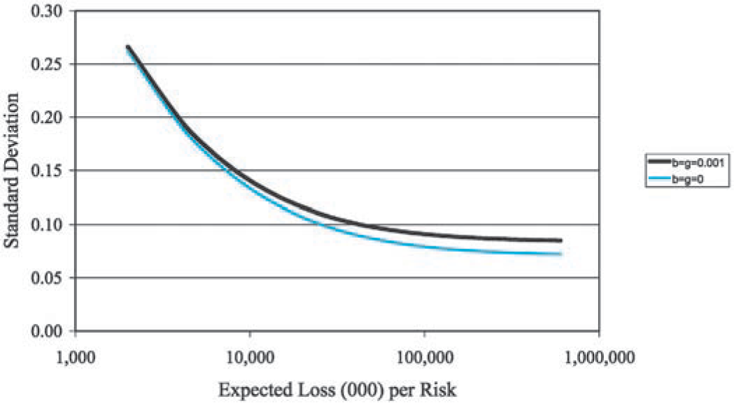
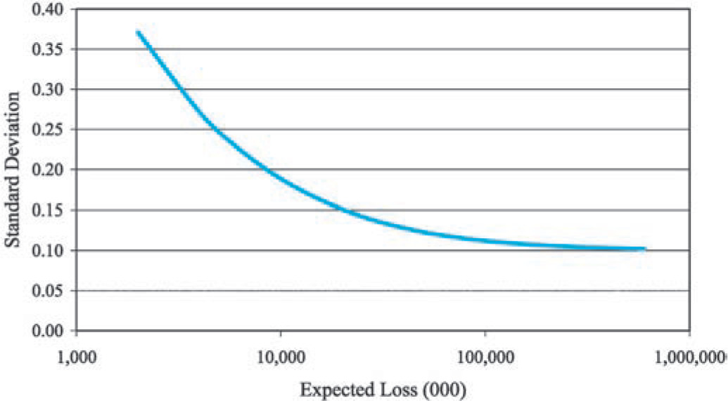
Equation (3.3) shows that the standard deviation of the normalized loss ratio, R = X/E[X] decreases asymptotically to $\sqrt{c}$ as we increase the size of the risk. Figure 5 illustrates this graphically.

$$\begin{array}{l} \text { Standard Deviation }[R]=\\ \frac{\sqrt{\lambda \cdot\left(\sigma^{2}+\mu^{2}\right)+c \cdot \lambda^{2} \cdot \mu^{2}}}{\lambda \cdot \mu} \underset{\lambda \rightarrow \infty}{\longrightarrow} \sqrt{c} . \end{array} \tag{3.3}$$

Figure 5.Standard deviation of normalized loss ratios for the collective risk model $\mu=15,000 \sigma=60,000$ $c=0.01$

4. Common shocks in the collective risk model

This section applies the ideas underlying the common shock model described in Section 2 to the collective risk model described in Section 3. Let us start with the claim count distributions.

Let $N_1$ and $N_2$ be two claim count random variables with $\mathrm{E}\left[N_i\right]=\lambda_i$ and $\operatorname{Var}\left[N_i\right]=\lambda_i+c_i$. $\lambda_i^2$ for $i=1$ and 2.

Let α be a random variable, which is independent of N₁ and N₂ with E[α] = 1 and Var[α] = g.

Let us now introduce common shocks into the joint distribution of N₁ and N₂ by selecting N₁ and N₂ from claim count distributions with means α · λ₁ and α · λ₂ and variances α · λ₁ + c₁ · (α · λ₁)² and α · λ₂ + c₂ · (α · λ₂)², respectively Let’s calculate the covariance matrix for N₁ and N₂.

Using Equation (2.2) to calculate the diagonal elements yields:

$$\begin{aligned} \operatorname{Var}\left[N_{i}\right] & =\mathrm{E}_{\alpha}\left[\operatorname{Var}\left[N_{i} \mid \alpha\right]\right]+\operatorname{Var}_{\alpha}\left[\mathrm{E}\left[N_{i} \mid \alpha\right]\right] \\ & =\mathrm{E}_{\alpha}\left[\alpha \cdot \lambda_{i}+c_{i} \cdot \alpha^{2} \cdot \lambda_{i}^{2}\right]+\operatorname{Var}_{\alpha}\left[\alpha \cdot \lambda_{i}\right] \\ & =\lambda_{i}+c_{i} \cdot \lambda_{i}^{2} \cdot(1+g)+\lambda_{i}^{2} \cdot g \\ & =\lambda_{i}+\lambda_{i}^{2} \cdot\left(c_{i}+g+c_{i} \cdot g\right). \end{aligned} \tag{4.1}$$

Using Equation (2.1) to calculate the off-diagonal elements yields:

$$\begin{aligned} \operatorname{Cov}\left[N_{1}, N_{2}\right]= & \mathrm{E}_{\alpha}\left[\operatorname{Cov}\left[N_{1}, N_{2} \mid \alpha\right]\right] \\ & +\operatorname{Cov}_{\alpha}\left[\mathrm{E}\left[N_{1} \mid \alpha\right], \mathrm{E}\left[N_{2} \mid \alpha\right]\right] \\ = & \mathrm{E}_{\alpha}[0]+\operatorname{Cov}_{\alpha}\left[\alpha \cdot \lambda_{1}, \alpha \cdot \lambda_{2}\right] \\ = & g \cdot \lambda_{1} \cdot \lambda_{2}. \end{aligned} \tag{4.2}$$

Now let’s add independent random claim severities, Z₁ and Z₂ to our common shock model. Here are the calculations for the elements of the covariance matrix for the total loss random variables X₁ and X₂:

$$\begin{aligned} \operatorname{Var}\left[X_{i}\right] & =\mathrm{E}_{N_{i}}\left[\operatorname{Var}\left[X_{i} \mid N_{i}\right]\right]+\operatorname{Var}_{N_{i}}\left[\mathrm{E}\left[X_{i} \mid N_{i}\right]\right] \\ & =\mathrm{E}_{N_{i}}\left[N_{i} \cdot \sigma_{i}^{2}\right]+\operatorname{Var}_{N_{i}}\left[N_{i} \cdot \mu_{i}\right] \\ & =\lambda_{i} \cdot \sigma_{i}^{2}+\mu_{i}^{2} \cdot\left(\lambda_{i}+\lambda_{i}^{2} \cdot\left(c_{i}+g+c_{i} \cdot g\right)\right) \\ & =\lambda_{i} \cdot\left(\sigma_{i}^{2}+\mu_{i}^{2}\right)+\lambda_{i}^{2} \cdot \mu_{i}^{2} \cdot\left(c_{i}+g+c_{i} \cdot g\right) . \end{aligned} \tag{4.3}$$

$$\begin{aligned} \operatorname{Cov}\left[X_{1}, X_{2}\right]= & \mathrm{E}_{\alpha}\left[\operatorname{Cov}\left[X_{1}, X_{2} \mid \alpha\right]\right] \\ & +\operatorname{Cov}_{\alpha}\left[\mathrm{E}\left[X_{1} \mid \alpha\right], \mathrm{E}\left[X_{2} \mid \alpha\right]\right] \\ = & \mathrm{E}_{\alpha}[0]+\operatorname{Cov}_{\alpha}\left[\alpha \cdot \lambda_{1} \cdot \mu_{1}, \alpha \cdot \lambda_{2} \cdot \mu_{2}\right] \\ = & g \cdot \lambda_{1} \cdot \mu_{1} \cdot \lambda_{2} \cdot \mu_{2}. \end{aligned} \tag{4.4}$$

Finally, let us multiply the claim severity random variables, Z₁ and Z₂, by a random variable, β with E[β] = 1 and Var[β] = b. Here are the calculations for the elements of the covariance matrix for the total loss random variables X₁ and X₂:

$$\begin{aligned} \operatorname{Var}\left[X_{i}\right]= & \mathrm{E}_{\beta}\left[\operatorname{Var}\left[X_{i} \mid \beta\right]\right]+\operatorname{Var}_{\beta}\left[\mathrm{E}\left[X_{i} \mid \beta\right]\right] \\ = & \mathrm{E}_{\beta}\left[\lambda_{i} \cdot \beta^{2} \cdot\left(\sigma_{i}^{2}+\mu_{i}^{2}\right)+\lambda_{i}^{2} \cdot \beta^{2} \cdot \mu_{i}^{2}\right. \\ & \left.\cdot\left(c_{i}+g+c_{i} \cdot g\right)\right]+\operatorname{Var}_{\beta}\left[\lambda_{i} \cdot \beta \cdot \mu_{i}\right] \\ = & \left(\lambda_{i} \cdot\left(\sigma_{i}^{2}+\mu_{i}^{2}\right)+\lambda_{i}^{2} \cdot \mu_{i}^{2} \cdot\left(c_{i}+g+c_{i} \cdot g\right)\right) \\ & \cdot \mathrm{E}\left[\beta^{2}\right]+\lambda_{i}^{2} \cdot \mu_{i}^{2} \cdot \operatorname{Var}[\beta] \\ = & \lambda_{i} \cdot\left(\mu_{i}^{2}+\sigma_{i}^{2}\right) \cdot(1+b)+\lambda_{i}^{2} \cdot \mu_{i}^{2} \\ & \cdot\left(c_{i}+g+b+c_{i} \cdot g+c_{i} \cdot b+g \cdot b\right. \\ & \left.+c_{i} \cdot g \cdot b\right). \end{aligned} \tag{4.5}$$

$$\begin{aligned} \operatorname{Cov}\left[X_{1}, X_{2}\right]= & \mathrm{E}_{\beta}\left[\operatorname{Cov}\left[X_{1}, X_{2} \mid \beta\right]\right] \\ & +\operatorname{Cov}_{\beta}\left[\mathrm{E}\left[X_{1} \mid \beta\right], \mathrm{E}\left[X_{2} \mid \beta\right]\right] \\ = & \mathrm{E}_{\beta}\left[g \cdot \lambda_{1} \cdot \beta \cdot \mu_{1} \cdot \lambda_{2} \cdot \beta \cdot \mu_{2}\right] \\ & +\operatorname{Cov}_{\beta}\left[\lambda_{1} \cdot \beta \cdot \mu_{1}, \lambda_{2} \cdot \beta \cdot \mu_{2}\right] \\ = & g \cdot \lambda_{1} \cdot \mu_{1} \cdot \lambda_{2} \cdot \mu_{2} \cdot \mathrm{E}\left[\beta^{2}\right] \\ & +\lambda_{1} \cdot \mu_{1} \cdot \lambda_{2} \cdot \mu_{2} \cdot \operatorname{Var}[\beta] \\ = & \lambda_{1} \cdot \mu_{1} \cdot \lambda_{2} \cdot \mu_{2} \cdot(b+g+b \cdot g) . \end{aligned} \tag{4.6}$$

The description of this version of the collective risk model can be completed with the following two assumptions:

1. b and g are the same for all risk sizes.

2. b and g are the same for all lines of insurance.

The parameters b and g represent parameter uncertainty that applies across lines of insurance, and it seems reasonable to assume that this uncertainty is independent of the size of risk. The second assumption keeps the math simple without sacrificing the main themes of this paper. Admittedly, there are many other assumptions one could make that are equally plausible. For example, the bs and gs could vary by line of insurance. In practice I have allowed g to vary by line of insurance. It is left as an exercise to the reader to show that you can replace g in Equations (4.4) and (4.6) with $\sqrt{g_{1} \cdot g_{2}}$ when the coefficient of correlation between α₁ and α₂ is equal to one.

The following example illustrates the implications of this model for normalized loss ratios as we vary the size of risk. The example will assume that μ = 16,000, σ = 60,000, and c = 0.010 for each line of insurance. The additional parameters will be b = g = 0.001. The final sections will show that these are reasonable choices of the parameters.

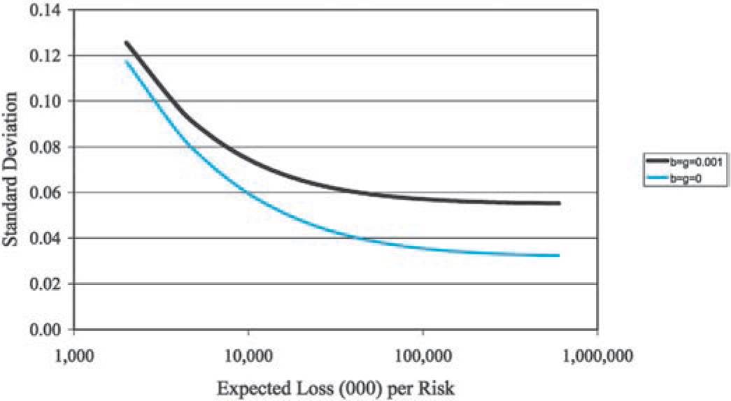
First let us note that since b and g are small compared to c, the introduction of b and g into the model has little effect on the standard deviation of the normalized loss ratio, although what effect there is increases with the size of the risk. This is illustrated by Figure 6.

Figure 6.Standard deviation of normalized loss ratios for the collective risk model $\mu=15,000 \sigma=60,000 c=0.01$

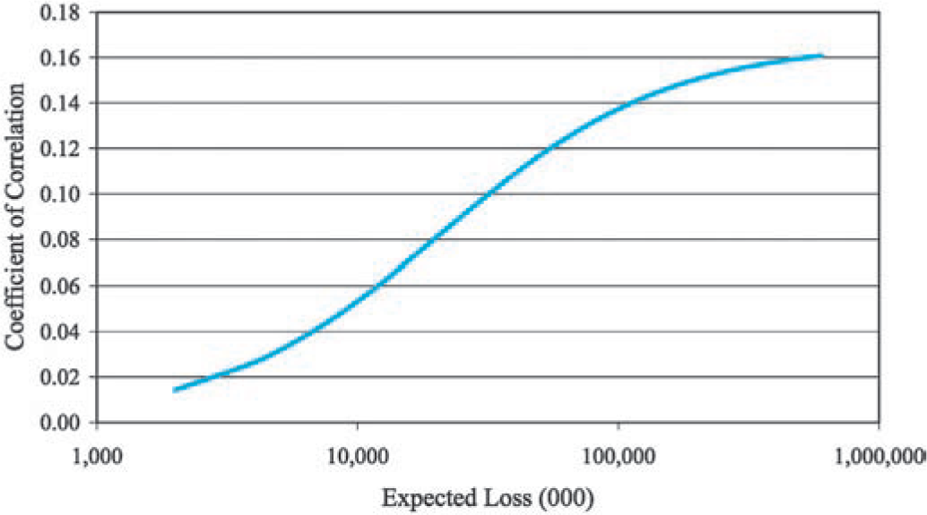
However, the coefficient of correlation between normalized loss ratios R₁ and R₂, as defined by

$$\rho\left[R_{1}, R_{2}\right]=\frac{\operatorname{Cov}\left[R_{1}, R_{2}\right]}{\sqrt{\operatorname{Var}\left[R_{1}\right] \cdot \operatorname{Var}\left[R_{2}\right]}},$$

increases significantly as you increase the size of the risk. In Figure 7, it is negligible for small risks.

Figure 7.Coefficient of correlation between normalized loss ratios of two equally sized risks for the collective risk model $\mu=15,000 \sigma=60,000 c=0.01 b=g=0.001$

Actuaries often find that their expectations of the coefficients of correlations are much higher. My best rationale for these expectations is that most expect a positive number between 0 and 1, and 0.5 seems like a good choice.

Even so, these (perhaps) seemingly small correlations can have a significant effect for a multiline insurer seeking to manage its risk as the following shall now illustrate.

Let us consider the covariance matrix for an insurer writing n lines of business:

$$\left(\begin{array}{cccc} \operatorname{Var}\left[X_{1}\right] & \operatorname{Cov}\left[X_{1}, X_{2}\right] & \cdots & \operatorname{Cov}\left[X_{1}, X_{n}\right] \\ \operatorname{Cov}\left[X_{2}, X_{1}\right] & \operatorname{Var}\left[X_{2}\right] & \cdots & \operatorname{Cov}\left[X_{2}, X_{n}\right] \\ \ldots & \ldots & \ldots & \ldots \\ \operatorname{Cov}\left[X_{n}, X_{1}\right] & \operatorname{Cov}\left[X_{n}, X_{2}\right] & \ldots & \operatorname{Var}\left[X_{n}\right] \end{array}\right)$$

The standard deviation of the insurer’s total losses, $X_1+\cdots+X_n$, is the square root of the sum of the elements of the covariance matrix. If $b=$ $g=0$, this sum consists of the $n$ variances along the diagonal. If $b$ or $g \neq 0$, then there are $n^2-n$ off-diagonal covariances included in the sum. As $n$ increases, so does the effect of even a “small” correlation. This is illustrated in Figures 8 and 9.

Figure 8.Standard deviation of normalized loss ratios for the collective risk model for the sum of two equally sized risks $\mu=15,000 \sigma=60,000 c=0.01$

Figure 9.Standard deviation of normalized loss ratios for the collective risk model for the sum of 10 equally sized risks $\mu=15,000 \sigma=60,000 c=0.01$

5. An empirical test of the model

The collective risk model, as defined above, makes predictions about how the volatility and correlation statistics of normalized loss ratios vary with insurer characteristics. These predictions should, at least in principle, be observable when one looks at a sizeable collection of insurance companies. This section will demonstrate that data that is publicly available from Schedule P is consistent with the major predictions of this model.

Data in Schedule P includes net losses, reported to date, and net premium by major line of insurance over a 10-year period. With Schedule P data for several insurers, various statistics such as standard deviations and coefficients of correlation between lines of insurance were calculated. Testing the model consisted of comparing these statistics with available information about each insurer.

Schedule P data presents several difficulties. The discussion that follows describes ways that Meyers, Klinker, and Lalonde (2003) dealt with these issues.

Schedule P premiums and reserves vary in largely predictable ways due to conditions that are present in the insurance market. These conditions are often referred to as the underwriting cycle. The underwriting cycle contributes an artificial volatility to underwriting results that lies outside the statistical realm of insurance risk. The measures insurance managers take to deal with the statistical realm of insurance risk, i.e., reinsurance and diversification, are different than those measures they take to deal with the underwriting cycle.

We dealt with the additional volatility caused by the underwriting cycle by using paid, rather than incurred, losses and estimating the ultimate incurred losses with industrywide paid loss development factors. We also attempted to smooth out differences in loss ratios that we deemed “predictable.” Appendix A in Meyers, Klinker, and Lalonde (2003)describes this process in greater detail.

After making the above adjustments, two other difficulties remain. First, the use of industrywide loss development factors removes the volatility that takes place after the report date of the loss. As such, we should expect the volatilities we measure to understate the ultimate volatility. To see this mathematically, consider Equation (2.2) with θ as a random variable representing future development. If we assume that the current loss estimates equal the expected ultimate loss, the second term in Equation (2.2) is the current variance, and the sum of the two terms is what we expect to be the ultimate variance.

Second, Schedule P losses are reported net of reinsurance. In addition, policy limits are not reported. Rather than incorporate this information directly into our estimation, we did sensitivity tests of our model, varying limits and reinsurance provisions within realistic scenarios. See Figures 10 and 11.

Figure 10.Commercial auto normalized loss ratios actual—Schedule P HiLim and LowLim from the collective risk model

Figure 11.Commercial auto normalized loss ratios simulated from collective risk model

This example presents results for commercial automobile liability insurance. I feel this is a good choice because: (1) it is a shorter tailed line than general liability and the underestimation of volatility will not be as great; (2) the use of reinsurance is not as great as it is in the general liability lines of insurance; and (3) commercial auto is not as prone to catastrophes as the property lines of insurance.

5.1. Standard deviation of normalized loss ratios vs. size of insurer

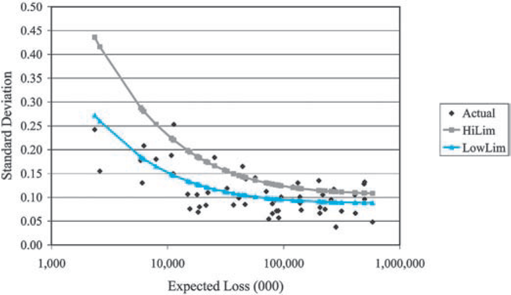
As illustrated in Figure 5, the collective risk model predicts that the standard deviation of insurer normalized loss ratios should decrease as the size of the insurer increases. In Figure 10 we can see that this prediction is consistent with the observed standard deviations calculated from the Schedule P data described above. In this figure we plotted the empirical standard deviation of 55 commercial auto insurers against the average (over the 10 years of reported data) expected loss for the insurer.^[2]

Figure 10 also includes the standard deviations predicted by the collective risk model. The series “LowLim” used claim severity distribution parameters taken from a countrywide ISO claim severity distributions evaluated at the $300,000 occurrence limit. In this series, c = 0.007, g = 0.0005, and b = 0, were selected judgmentally. See Section 6 for commentary on selecting b and g.

Now we (at ISO) know from data reported to us that, depending on the subline (e.g., light and medium trucks or long-haul trucks), typically 65% to 90% of all commercial auto insurance policies are written at the $1 million policy limit. But since I also believed that the Schedule P data understates the true volatility of the normalized loss ratios, I selected the $300,000 policy limit for the test.

For the sake of comparison, the series “HiLim” represents a judgmental adjustment that one might use to account for problems with the Schedule P data. Claim severity distribution parameters were taken from countrywide ISO claim severity distributions evaluated at the $1 million occurrence limit. In this series c = 0.010, g = 0.0010, and b = 0 were selected judgmentally.

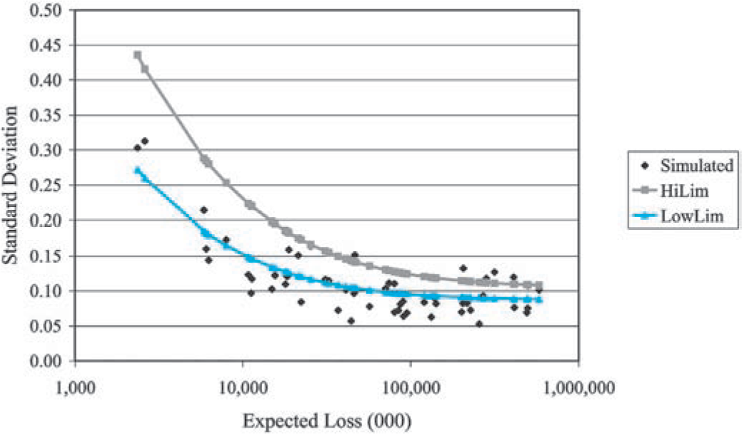
Figures 10 and 11 also provide a comparable plot of normalized loss ratios simulated from a collective risk model, one per insurer, using the same parameters used for the “LowLim” and “HiLim” series. The two plots suggest that the Schedule P data is well represented by the collective risk model—for an individual line of insurance.

5.2. Coefficients of correlation vs. the size of the insurer

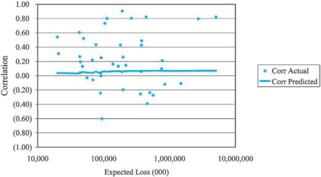
As Figure 7 illustrates, a second prediction of the collective risk model is that the coefficients of correlation will increase with the size of the insurer. In Figure 12, we plotted the empirical coefficients of correlation between commercial auto and personal auto for 38 insurers of both lines against the average (over 10 years of experience reported for the two lines of insurance) expected loss. A comparable plot based on simulated data from the underlying model is in Figure 13.^[3]

Figure 12.Commercial auto and personal auto normalized loss ratios actual—Schedule P, predicted—collective risk model

Figure 13.Commercial auto and personal auto normalized loss ratios simulated and predicted from the collective risk model

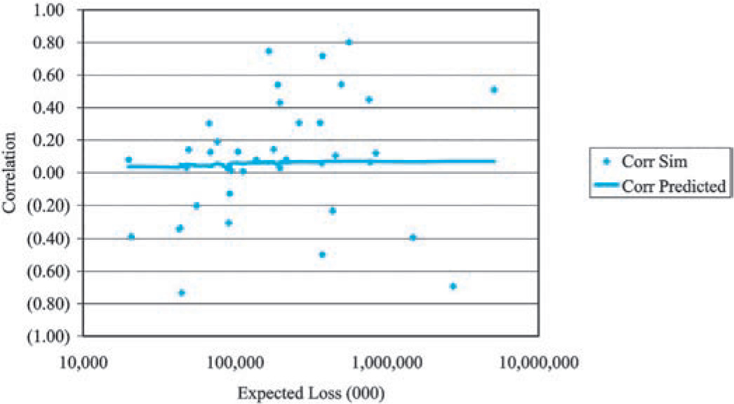
We observe that the coefficient of correlation is a very volatile statistic for both the empirical data and the simulated data which has a built-in assumption consistent with our hypothesis. This serves to illustrate the difficulty in measuring the effect of correlation in insurance data.

To provide a deeper analysis of the correlation problem, assume that the common shock random variables α and β operate on all insurers simultaneously. For random normalized loss ratios R₁ and R₂ the covariance is calculated as

$$\mathrm{E}\left[\left(R_{1}-1\right) \cdot\left(R_{2}-1\right)\right]=\frac{\operatorname{Cov}\left[X_{1}, X_{2}\right]}{\lambda_{1} \cdot \mu_{1} \cdot \lambda_{2} \cdot \mu_{2}}=b+g+b \cdot g ;\tag{5.1}$$

which is derived from Equation (4.5).

Now as already established, the standard deviation of the normalized loss ratios decreases with the size of the insurer. Thus the denominator of:

$$\rho\left[R_{1}, R_{2}\right]=\frac{\mathrm{E}\left[\left(R_{1}-1\right) \cdot\left(R_{2}-1\right)\right]}{\operatorname{Std}\left[R_{1}\right] \cdot \operatorname{Std}\left[R_{2}\right]}$$

should decrease. If we can demonstrate with the Schedule P data that the numerator does not decrease, we can conclude that the prediction that coefficients of correlation will increase is consistent with the Schedule P data. It is to this demonstration that we now turn.

In the test that (R₁ − 1) · (R₂ − 1) was independent of insurer size the data consisted of all 15,790 possible pairs of r₁ and r₂, and the associated expected losses, taken from the same year and different insurers. The line^[4] fit to the ordered pairs

$$\text { (Average Size of the Insurer, }\left(r_{1}-1\right) \cdot\left(r_{2}-1\right) \text { ) }$$

produced a slope of +1.95 × 10⁻¹⁰. This slightly positive slope means that an increasing coefficient of correlation is consistent with the Schedule P data.

Equation (5.1) also provides us with a way to estimate the quantity b + g + b · g. One simply has to calculate the weighted average of the 15,790 products of (r₁ − 1) · (r₂ − 1) = 0.00054. Since the 15,790 observations are not independent, the usual tests of statistical significance do not apply. To test the statistical significance of this result, 200 weighted averages were simulated using the “LowLim” parameters (except that b = g = 0) with the result that the highest weighted average was 0.000318. Since the final weighted average of 0.00054 is greater than all the simulations generated under the null hypothesis that b + g + b · g = 0, the result is statistically significant.

One final simulation with the “LowLim” parameters (except that b = 0 and g = 0.00054) calculated 200 slopes results in a slope of 1.95 × 10⁻¹⁰, which was just below the 49th highest. Thus the fitted slope would not be unusual if the collective risk model is the correct model.

6. The role of judgment in selecting final parameters

Historically, most actuaries have resorted to judgment in the quantification of correlation. This paper was written in the hope of supplying some objectivity to this quantification. ISO has worked on quantifying this correlation. ISO has conducted analyses similar to the one described above for several lines of business using both Schedule P data and individual insurer data reported to ISO. In the end, no data set is perfect for the job, and some judgments must be made. Here are some of the considerations made in selecting the final models. Comments are always welcome.

• First of all, the selection of the model itself is subject to judgment. As noted above, there are other ways of introducing the “common shock idea” that are very likely to be consistent with the data.

• We have reason to believe that the data we observe understates the ultimate variability since there are some claims that have yet to be settled. As a result we judgmentally increased the c, b, and g parameters in the final model.

• Since the estimation procedure described provides an estimate of b + g + b · g, it is impossible to distinguish between the claim frequency common shocks as quantified by g, and the claim severity common shocks as quantified by b. A lot of work has been done with claim severity and claim frequency trend, and one can look to uncertainties in these trends when selecting the final parameters.

Accounting data such as Schedule P may not be the best source for such analyses, but if we cannot see the effect of correlation in the accounting data, I would ask, do we need to worry about correlation? I believe that the analysis in this paper demonstrates that we do need to consider correlation between lines of insurance.