On the Subadditivity of Tail Value at Risk: An Investigation with Copulas

1. Introduction

Assume that the loss incurred by an insurance company is given by the realization of a random variable X, defined on a probability space (Ω,𝓕,ℙ). To protect the insured, regulators demand that the insurance company hold an amount of money large enough to be able to compensate the policyholders with a high probability. Obviously, a fraction of that amount is provided by the premiums paid by the policyholders. The missing amount is provided by the shareholders who put money at risk in the insurance company. They demand a certain return on this capital.

In this paper, we will concentrate on measures to calculate the required solvency level. Because this has obvious connections with the right tail of the random variable representing the loss, a risk measure based on quantiles seems to be adequate. Quantiles have been called Value at Risk (VaR) by bankers for a long time and we will follow this terminology here. The VaR at the level p is given by:

\[ \operatorname{VaR}_{p}[X]=\inf \left\{x \in \mathbb{R} \mid F_{X}(x) \geq p\right\}, \quad 0<p<1, \]

where F_X(x) = ℙ[X ≤ x] is the cumulative density function of X. More generally, we will resort to risk measures to determine the required solvency level. Therefore, let (Ω,𝓕,ℙ) be a probability space and let Γ be a nonempty set of 𝓕-measurable random variables. A risk measure ρ is a functional:

\[ \rho: \Gamma \rightarrow \mathbb{R} \cup\{\infty\} . \]

Let us now analyze the situation when we merge two risks X₁ and X₂. The regulator wants to minimize the shortfall risk:

\[ (X-\rho[X])_{+}=\max (0, X-\rho[X]) . \]

For a merger, the following inequality holds with probability one (Dhaene et al. 2008):

\[ \begin{array}{l} \left(X_{1}+X_{2}-\rho\left[X_{1}\right]-\rho\left[X_{2}\right]\right)_{+} \\ \quad \leq\left(X_{1}-\rho\left[X_{1}\right]\right)_{+}+\left(X_{2}-\rho\left[X_{2}\right]\right)_{+} . \end{array} \tag{1.1} \]

Therefore, from the viewpoint of avoiding shortfall, the aggregation of risk is to be preferred in the sense that the shortfall decreases. The underlying reason is that within the merger, the shortfall of one of the entities can be compensated by potentially better results for the other.

However, when investors have an amount of capital ρ[X₁] + ρ[X₂], they will prefer investing in two separate companies because the following inequality holds with probability one:

\[ \begin{array}{l} \left(\rho\left[X_{1}\right]+\rho\left[X_{2}\right]-X_{1}-X_{2}\right)_{+} \\ \quad \leq\left(\rho\left[X_{1}\right]-X_{1}\right)_{+}+\left(\rho\left[X_{2}\right]-X_{2}\right)_{+} . \end{array} \]

Investors will get a higher return by investing in two separate companies due to the firewalls that exist between X₁ and X₂. Indeed, if for one of the separate companies X₁ − ρ[X₁] > 0, this will not affect Company 2. For a merger, however, if ρ[X₂] − X₂ > 0 and X₁ − ρ[X₁] > 0, a part of the capital invested in Company 2 will be used to compensate the bad results for Company 1. Investors may have incentives to invest in the merger once:

\[ \rho\left[X_{1}+X_{2}\right] \leq \rho\left[X_{1}\right]+\rho\left[X_{2}\right] . \tag{1.2} \]

A risk measure ρ that conforms to (1.2) for all X₁,X₂ ∈ Γ is said to be subadditive. On the other hand, a risk measure is superadditive when for all X₁,X₂ ∈ Γ:

\[ \rho\left[X_{1}+X_{2}\right] \geq \rho\left[X_{1}\right]+\rho\left[X_{2}\right] . \]

It is well known that the VaR is not subadditive. Therefore, we will look for other risk measures that are subadditive. For such a risk measure, we do not necessarily have that

\[ \begin{aligned} \left(X_{1}+\right. & \left.X_{2}-\rho\left[X_{1}+X_{2}\right]\right)_{+} \\ & \leq\left(X_{1}-\rho\left[X_{1}\right]\right)_{+}+\left(X_{2}-\rho\left[X_{2}\right]\right)_{+} \end{aligned} \tag{1.3} \]

for all outcomes of X₁ and X₂. Of course, when ρ is superadditive, (1.3) is fulfilled for all outcomes of X₁ and X₂. However, for the reasons given above, superadditive risk measures will not motivate investors.

As mentioned in Dhaene et al. (2008), if for a given random couple (X₁,X₂) we have that ℙ[X₁ > ρ[X₁],X₂ > ρ[X₂]] > 0 and that equation (1.3) is satisfied for all outcomes of X₁ and X₂, then we need to have that ρ[X₁ + X₂] ≥ ρ[X₁] + ρ[X₂]. Therefore, a subadditive risk measure satisfying (1.3) for every outcome of all random couples (X₁,X₂) needs to be additive for all random couples for which ℙ[X₁ > ρ[X₁],X₂ > ρ[X₂]] > 0. Only for random couples with ℙ[X₁ > ρ[X₁],X₂ > ρ[X₂]] = 0, could a credit be given for the capital requirement of the merger. Hence, condition (1.3) limits the range of possible risk measures considerably.

Dhaene et al. (2008) analyzed the effect of weakening the condition that ρ should satisfy inequality (1.3) for any outcome of all random couples (X₁,X₂) to the requirement that couples on average satisfy (1.3)

\[ \begin{aligned} \mathbb{E}\left(X_{1}\right. & \left.+X_{2}-\rho\left[X_{1}+X_{2}\right]\right)_{+} \\ & \leq \mathbb{E}\left(X_{1}-\rho\left[X_{1}\right]\right)_{+}+\mathbb{E}\left(X_{2}-\rho\left[X_{2}\right]\right)_{+} \end{aligned} \tag{1.4} \]

for all random couples (X₁,X₂). They showed that all translation invariant and positively homogeneous risk measures satisfy condition (1.4) for every bivariate normal distribution and more generally, for every bivariate elliptical distribution. A risk measure is said to be translation invariant if for all b ∈ ℝ and for each random variable X ∈ Γ we have that ρ[X + b] = ρ[X] + b. A positively homogeneous risk measure satisfies ρ[aX] = aρ[X] for all a > 0 and X ∈ Γ. Now suppose a risk measure is translation invariant, positively homogeneous and subadditive. If it also satisfies the property that for all X₁,X₂ ∈ Γ with ℙ[X₁ ≤ X₂] = 1 we have that ρ[X₁] ≤ ρ[X₂] (monotonicity), it is said to be coherent in the sense of Artzner et al. (1999).

Although there exist several coherent risk measures, we will focus in the present paper on the TVaR only. This is undoubtedly the most popular coherent risk measure in practice. The TVaR of a random variable X is defined as

\[ \operatorname{TVaR}_{p}[X]=\frac{1}{1-p} \int_{p}^{1} \operatorname{VaR}_{q}[X] d q, \quad 0<p<1 \]

where p is a given confidence level. TVaR at a level p is equal to the average of all quantiles of X above the p-quantile. This gives it, just like the VaR, a nice intuitive interpretation. The TVaR, as we define it, is related to the expected shortfall as defined in Acerbi and Tasche (2002). These authors see losses as a negative outcome of a random variable and hence look at the left-hand side of the distribution. For continuous random variables, the TVaR is equal to the conditional tail expectation (CTE), which is defined as

\[ \mathrm{CTE}_{p}[X]=\mathbb{E}\left[X \mid X>\operatorname{VaR}_{p}[X]\right], \quad 0<p<1 . \]

The CTE is not subadditive (see Dhaene et al. 2008). As shown in Dhaene et al. (2008), examples can be constructed for which (1.4) does not hold for the TVaR. Hence, TVaR can be too subadditive in the sense of condition (1.4).

The purpose of this paper is twofold. On the one hand, we want to show that the TVaR is able to deal in an appropriate fashion with the diversification benefit of a merger under a wide range of dependence structures and margins. In our examples, we will observe that the TVaR only gives a credit for diversification when appropriate, thereby providing a framework for compromise between the expectations of the investors and those of the regulator. On the other hand, by taking a practical approach based on copulas to describe the dependence structure between the margins, we want to learn more about the behavior of different copulas with respect to the diversification benefit. Copulas have been gaining a lot of interest in insurance applications [e.g., Frees and Valdez (1998), Venter (2001), and Blum, Dias, and Embrechts (2002)] and in other research areas. This has been the cause for some warnings and discussion lately [Mikosch (2006) and the subsequent discussion papers].

The rest of the paper is organized as follows. In Section 2, we define some measures to compare the residual risk of a conglomerate and of standalone companies. We illustrate the effect of merging independently and identically distributed exponential subsidiaries on these measures when TVaR is used as a risk measure. In Section 3, we define the concept of a copula and the copulas which are used in this paper. Some well-known dependence measures are defined in Section 4, where we also make a graphical analysis of some copulas. In Section 5, we then analyze the residual risk of a conglomerate and a group of standalone companies based on a simulation study. We again use TVaR to determine the required solvency level. We conclude in Section 6.

2. Residual risk of conglomerate and standalones

Assume the risks X_i with i ∈ {1, . . . ,K}. For the conglomerate \(X=\sum_{i=1}^K X_i\), we will compute the mean, the variance, the skewness, and the kurtosis of the residual risk RR_X = (X − ρ[X])₊:

\[ \begin{aligned} \mathbb{E}\left[R R_{X}\right]= & \int_{\rho[X]}^{+\infty}(x-\rho[X]) f_{X}(x) d x, \\ \operatorname{Var}\left[R R_{X}\right]= & \sigma^{2}\left[R R_{X}\right] \\ = & \int_{0}^{+\infty}\left((x-\rho[X])_{+}-\mathbb{E}\left[R R_{X}\right]\right)^{2} \\ & \times f_{X}(x) d x, \\ \gamma\left[R R_{X}\right]= & \frac{1}{\mathbb{V a r}\left[R R_{X}\right]^{3 / 2}} \int_{0}^{+\infty} \\ & \times\left((x-\rho[X])_{+}-\mathbb{E}\left[R R_{X}\right]\right)^{3} f_{X}(x) d x, \\ \kappa\left[R R_{X}\right]= & \frac{1}{\mathbb{V a r}\left[R R_{X}\right]^{2}} \int_{0}^{+\infty} \\ & \times\left((x-\rho[X])_{+}-\mathbb{E}\left[R R_{X}\right]\right)^{4} f_{X}(x) d x . \end{aligned} \]

For each of the entities X_i looked at as standalones, we assume we use the same risk measure ρ to determine the solvency level. Hence, we can write the mean, variance, skewness, and kurtosis of the residual risk \(R R_{X_i}=\left(X_i-\rho\left[X_i\right]\right)_{+}\) as

\[ \begin{aligned} \mathbb{E}\left[R R_{X_{i}}\right]= & \int_{\rho\left[X_{i}\right]}^{+\infty}\left(x-\rho\left[X_{i}\right]\right) f_{X_{i}}(x) d x \\ \operatorname{Var}\left[R R_{X_{i}}\right]= & \sigma^{2}\left[R R_{X_{i}}\right] \\ = & \int_{0}^{+\infty}\left(\left(x-\rho\left[X_{i}\right]\right)_{+}-\mathbb{E}\left[R R_{X_{i}}\right]\right)^{2} \\ & \times f_{X_{i}}(x) d x \\ \gamma\left[R R_{X_{i}}\right]= & \frac{1}{\mathbb{V a r}\left[R R_{X_{i}}\right]^{3 / 2}} \int_{0}^{+\infty} \\ & \times\left(\left(x-\rho\left[X_{i}\right]\right)_{+}-\mathbb{E}\left[R R_{X_{i}}\right]\right)^{3} \\ & \times f_{X_{i}}(x) d x \\ \kappa\left[R R_{X_{i}}\right]= & \frac{1}{\mathbb{V a r}\left[R R_{X_{i}}\right]^{2}} \int_{0}^{+\infty} \\ & \times\left(\left(x-\rho\left[X_{i}\right]\right)_{+}-\mathbb{E}\left[R R_{X_{i}}\right]\right)^{4} \\ & \times f_{X_{i}}(x) d x \end{aligned} \]

We denote

\[ \begin{aligned} \mu_{3}\left[R R_{X_{i}}\right]= & \int_{0}^{+\infty}\left(\left(x-\rho\left[X_{i}\right]\right)_{+}-\mathbb{E}\left[R R_{X_{i}}\right]\right)^{3} \\ & \times f_{X_{i}}(x) d x \end{aligned} \]

and

\[ \begin{aligned} \mu_{4}\left[R R_{X_{i}}\right]= & \int_{0}^{+\infty}\left(\left(x-\rho\left[X_{i}\right]\right)_{+}-\mathbb{E}\left[R R_{X_{i}}\right]\right)^{4} \\ & \times f_{X_{i}}(x) d x \end{aligned} \]

In the case that the risks X_i are identically and independently distributed, the mean, variance, skewness, and kurtosis of the sum of the residual risk of the separate entities, \(R R_{X_{1 ; K}}=\) Σ^K_i=1 \(\sum_{i=1}^K\left(X_i-\rho\left[X_i\right]\right)_{+}\), can be written as follows:

\[ \begin{aligned} \mathbb{E}\left[R R_{X_{1 ; K}}\right] & =\sum_{i=1}^{K} \mathbb{E}\left[R R_{X_{i}}\right] \\ \operatorname{Var}\left[R R_{X_{1 ; K}}\right] & =\sigma^{2}\left[R R_{X_{1 ; K}}\right]=\sum_{i=1}^{K} \operatorname{Var}\left[R R_{X_{i}}\right] \\ \gamma\left[R R_{X_{1 ; K}}\right] & =\frac{\sum_{i=1}^{K} \mu_{3}\left[R R_{X_{i}}\right]}{\operatorname{Var}\left[R R_{X_{1 ; K}}\right]^{3 / 2}} \\ \kappa\left[R R_{X_{1 ; K}}\right] & =\frac{\sum_{i=1}^{K} \mu_{4}\left[R R_{X_{i}}\right]}{\operatorname{Var}\left[R R_{X_{1 ; K}}\right]^{2}} \end{aligned} \]

In the more general case, the variance, skewness, and kurtosis of the sum of the residual risk of the separate entities and the distribution of the loss of the merger depend on the dependence structure and the marginal distributions of each of the entities. In such cases, we will use a simulation model. As a basis for comparison for the results generated through simulation, we first assume the subsidiaries are all identically and independently exponentially distributed, since this allows us to use explicit formulas and numerical approximation methods.

If \(X_{i} \stackrel{\mathrm{iid}}{\sim} \operatorname{Expo}(\lambda)\) for i ∈ {1,2}, i.e.,

\[ F_{X_{i}}(x)=1-e^{-\lambda x}, \quad \text { for } \quad x>0 \quad \text { and } \quad \lambda>0, \]

then it is well known that 𝔼[X_i] = σ[X_i] = 1/λ and that X = X₁ + X₂ ~ Gamma(α = 2, β = λ), where the distribution function of a Gamma(α,β)-distributed random variable X is given by

\[ \begin{array}{l} F_{X}(x)=\int_{0}^{x} \frac{\beta^{\alpha}}{\Gamma(\alpha)} y^{\alpha-1} e^{-\beta y} d y\\ \text { for } \quad x>0, \quad \alpha>0 \quad \text { and } \quad \beta>0 \text {, } \end{array} \]

where Γ(α) denotes the Gamma-function. Because the α-parameter is an integer, we in fact have the Erlang Distribution.

The VaR and TVaR for an exponential distribution are given by

\[ \begin{aligned} \operatorname{VaR}_{p}\left[X_{i}\right] & =-\frac{\ln (1-p)}{\lambda}, \\ \operatorname{TVaR}_{p}\left[X_{i}\right] & =\frac{1}{\lambda}+\operatorname{VaR}_{p}\left[X_{i}\right]=\frac{1}{\lambda}(1-\ln (1-p)) . \end{aligned} \]

In general, the VaR for the gamma distribution has no closed form but good numerical approximations are available in a lot of statistical software packages. As shown in Landsman and Valdez (2004), if X ~ Gamma(α,β), we have that

\[ \operatorname{TVaR}_{p}[X]=\frac{\alpha\left(1-F_{Y}\left(\operatorname{VaR}_{p}[X]\right)\right)}{\beta(1-p)} \]

where Y ~ Gamma(α + 1,β).

Now assume that X₁ and X₂ are i.i.d. according to the exponential distribution with parameter λ = 1/50. Then we have that TVaR_0.95[X_i] = 200, for i ∈ {1,2}, and TVaR_0.95[X] = 296 and that TVaR_0.99[X_i] = 280, for i ∈ {1,2}, and TVaR_0.99[X] = 388. For the residual risk, when taking the TVaR at a 95% and 99% level, we find the risk measures as summarized in Table 1.

Both at the 95% and 99% level, we observe that even though the TVaR for the conglomerate is considerably lower than the sum of the solvency levels of the two separate entities, the mean and the standard deviation of the residual risk of the conglomerate are considerably lower than for the sum of the separate entities. The skewness and the kurtosis of the residual risk for the merger are larger than for the two separate entities. The probability of default for the merger is considerably lower. This illustrates that due to the diversification benefit given by Equation (1.1) and allowing for the subadditivity implicit to the TVaR, the conglomerate performs better both with respect to the mean and the standard deviation of the residual risk.

We make the same exercise at a 99% confidence level for a merger of 5 and of 10 independent risks with Expo(1/50)-distribution margins. We then have TVaR_0.99[Σ⁵_i=1 X_i] = 650 and TVaR_0.99[Σ¹⁰_i=1X_i] = 1024. The results are given in Table 2.

In Table 2, we observe that for the conglomerate, the expectation and standard deviation of the residual risk increase about 20% when the number of subsidiaries is increased from 5 to 10. For the separate entities, however, these measures increase 100% and 41%, respectively. This example shows the interest in merging risks and that the TVaR is not too subadditive, if we are interested in these measures of the residual risk. Of course, the probability that at least one of the subsidiaries defaults increases when the number of subsidiaries increases. For the conglomerate, however, this probability remains (nearly) constant, showing that the subadditivity of the TVaR does not increase the default probability for the merger in this example. The skewness and kurtosis for the merger decrease only slowly when moving from 5 to 10 dimensions. These risk measures are significantly larger when the companies are separated. This is, however, a simple consequence of the fact that the distribution of the residual risk for the merger has a probability of being zero, which is a lot more important. Therefore, this should not be a reason to conclude that the TVaR is too subadditive.

In what follows, we use the average residual risk and the probability that the residual risk is zero to assess whether the subadditivity of the TVaR is acceptable. We also assess what happens with the standard deviation of the residual risk for the merger and the sum of the standalones.

3. Copulas

3.1. Definition and existence

The notion of copula was introduced by Sklar (1956). We define a d-dimensional copula.

Definition 1 (Multivariate Copula). A d-dimensional copula C is a nondecreasing right-continuous function from the unit cube [0,1]^d to the unit interval [0,1] which satisfies the following properties:

1. C(u₁, . . . ,u_i−1,0,u_i+1, . . . ,u_d) = 0 for i ∈ {1, . . . ,d},

2. C(1, . . . ,1,u_i,1, . . . ,1) = u_i for i ∈ {1, . . . ,d},

3. For all (a₁, . . . ,a_d) and (b₁, . . . ,b_d) in [0,1]^d with a_i < b_i for i ∈ {1, . . . ,d}:

   \[ \begin{array}{l} \Delta_{a_{1}, b_{1}} \ldots \Delta_{a_{d}, b_{d}} C\left(u_{1}, \ldots, u_{d}\right) \geq 0\\ \text { for all }\left(u_{1}, \ldots, u_{d}\right) \in[0,1]^{d}, \end{array} \tag{3.1} \]

   where

   \[ \begin{array}{l} \Delta_{a_{i}, b_{i}} C\left(u_{1}, \ldots, u_{d}\right)= \\ \quad C\left(u_{1}, \ldots, u_{i-1}, b_{i}, u_{i+1}, \ldots, u_{d}\right) \\ \quad-C\left(u_{1}, \ldots, u_{i-1}, a_{i}, u_{i+1}, \ldots, u_{d}\right) . \end{array} \]

A copula can be interpreted as the joint distribution function of a random vector on the unit cube. Note that condition (3.1) in Definition 1 ensures that

\[ \mathbb{P}\left[a_{1} \leq U_{1} \leq b_{1}, \ldots, a_{d} \leq U_{d} \leq b_{d}\right] \geq 0 \]

for all (a₁, . . . ,a_d) and (b₁, . . . ,b_d) in [0,1]^d with a_i < b_i for i ∈ {1, . . . ,d} and where (U₁, . . . ,U_d) denotes a d-dimensional uniform random vector with copula C.

It follows from the next theorem that the joint distribution function of a continuous random vector can be written as a function of its margins and a unique copula.

Theorem 1 (Sklar’s Theorem in d-dimensions). Let F be a d-dimensional distribution function with marginal distribution functions F₁, . . . ,F_d. Then there is a d-dimensional copula C such that for all x ∈ ℝ^d

\[ F\left(x_{1}, \ldots, x_{d}\right)=C\left(F_{1}\left(x_{1}\right), \ldots, F_{d}\left(x_{d}\right)\right) . \tag{3.2} \]

If F₁, . . . ,F_d are all continuous, then C is unique. Conversely, if C is a d-dimensional copula, and F₁, . . . ,F_d are distribution functions, then F defined by (3.2) is a d-dimensional distribution with margins F₁, . . . ,F_d.

See Nelsen (1999) for a proof.

3.2. Examples of copulas

Every d-dimensional copula C satisfies the inequality

\[ \begin{aligned} \max & \left\{0, \sum_{i=1}^{d} u_{i}-(n-1)\right\} \leq C\left(u_{1}, \ldots, u_{d}\right) \\ & \leq \min \left\{u_{1}, \ldots, u_{d}\right\} \\ & \text { for all }\left(u_{1}, \ldots, u_{d}\right) \in[0,1]^{d} \end{aligned} \tag{3.3} \]

For d ≥ 3, the left-hand side of (3.3) does not satisfy the condition for being a copula [see Denuit et al. (2005) for an explanation]. In dimension 2, the left-hand side of (3.3) is called the Fréchet lower bound copula, which we denote with C_L. Random couples with this copula are said to be countermonotonic. The right-hand side of (3.3) is the d-dimensional Fréchet upper bound copula, which we denote with C_U. Random vectors with this copula are said to be comonotonic. Comonotonicity is the strongest possible dependence.

Below, we define some other well known copulas:

• The independence copula

  For d independent random variables X₁, . . . ,X_d with respective distribution functions F₁, . . . ,F_d, the joint distribution function is equal to Π^d_i=1F_i(x_i). Therefore, the copula underlying independent risks is given by \[\begin{aligned}C_{I}\left(u_{1}, \ldots, u_{d}\right)= & \prod_{i=1}^{d} u_{i} \\ & \text { for all }\left(u_{1}, \ldots, u_{d}\right) \in[0,1]^{d} . \end{aligned}\]

• The survival copula or flipped copula

  Let C be a d-dimensional copula and let (U₁, . . . ,U_d) be a uniform random vector on [0,1]^d with copula C. The survival function is defined and denoted with \[\begin{aligned} C_{S}\left(u_{1}, \ldots, u_{d}\right)= & \mathbb{P}\left[U_{1}>u_{1}, \ldots, U_{d}>u_{d}\right] \\ & \text { for all }\left(u_{1}, \ldots, u_{d}\right) \in[0,1]^{d} .\end{aligned}\]

  C_S is not a copula since C_S(0, . . . ,0) = 1. However, \[\begin{aligned} \bar{C}\left(u_{1}, \ldots, u_{d}\right)= & C_{S}\left(1-u_{1}, \ldots, 1 u_{d}\right) \\ & \text { for all }\left(u_{1}, \ldots, u_{d}\right) \in[0,1]^{d} \end{aligned}\]

  is a copula, which we call the survival copula or the flipped copula of the copula C. If (U₁, . . . ,U_d) is a uniform random vector on [0,1]^d with copula C, then (1 − U₁, . . . ,1 − U_d) is a uniform random vector on [0,1]^d with copula C̅.

• The normal copula

  The d-dimensional random vector X = (X₁, . . . , X_d)^t has a multivariate normal distribution with mean vector μ = (μ₁, . . . ,μ_d) and positive-definite dispersion matrix Σ if its distribution function is given by \[\begin{aligned} \nu_{\mu, \Sigma}(\mathbf{x})= & \int_{-\infty}^{x_{1}} \cdots \int_{-\infty}^{x_{d}} \frac{1}{\sqrt{(2 \pi)^{d}|\Sigma|}} \\ & \times \exp \left(-\frac{1}{2}(\boldsymbol{\epsilon} \boldsymbol{\mu})^{t} \Sigma^{-1}(\boldsymbol{\epsilon}-\boldsymbol{\mu})\right) d \epsilon_{1} \ldots d \epsilon_{d} \end{aligned} \]

  where ε = (ε₁, . . . , ε_d)^t and x = (x₁, . . . ,x_d)^t. Note that for the normal distribution, Σ = ℂov[X], where ℂov [X] denotes the variance-covariance matrix of X. It follows from Sklar’s theorem that this multivariate distribution gives rise to a unique copula. The copula of a random vector is invariant under strictly increasing transformations of the random vector (Nelsen 1999). Therefore, the copula of a v_μ,Σ-distribution is identical to that of a v ₀,_P-distribution, where P is the correlation matrix implied by the dispersion matrix Σ. In what follows, we will implicitly assume that Σ refers to the correlation matrix and we will work with the standardized version of the multivariate normal distribution, denoted with v_Σ. The d-dimensional normal copula with correlation matrix Σ is then defined and denoted by \[\begin{aligned} C_{\Sigma}\left(u_{1}, \ldots, u_{d}\right)= & \nu_{\Sigma}\left(\Phi^{-1}\left(u_{1}\right), \ldots, \Phi^{-1}\left(u_{d}\right)\right) \\ & \text { for all }\left(u_{1}, \ldots, u_{d}\right) \in[0,1]^{d} \end{aligned} \]

  where Φ denotes the distribution function of the univariate standard normal distribution. A simulation algorithm for the normal copula can be found in Wang (1999) or in Embrechts, Lindskog, and McNeil (2003).

• The Student copula

  The d-dimensional random vector X = (X₁, . . . ,X_d)^t has a (nonsingular) multivariate Student distribution with m degrees of freedom (m > 0), mean vector μ, and positive-definite dispersion matrix Σ if its distribution function is given by \[\begin{aligned} & t_{m, \mu, \Sigma}(\mathbf{x}) \\ & =\int_{-\infty}^{x_1} \cdots \int_{-\infty}^{x_d} \frac{\Gamma\left(\frac{m+d}{2}\right)|\Sigma|^{-1 / 2}}{\Gamma\left(\frac{m}{2}\right)(m \pi)^{d / 2}} \\ & \quad \times\left[1+\frac{1}{m}(\epsilon-\mu)^t \Sigma^{-1}(\epsilon-\mu)\right]^{-(m+d) / 2} d \epsilon_1 \ldots d \epsilon_d \end{aligned} \]

  where ε = (ε₁, . . . , ε_d)^t and x = (x₁, . . . ,x_d)^t. The multivariate Student distribution with m = 1 is also called the multivariate Cauchy distribution. Note that for the Student distribution with m degrees of freedom (m > 2), we have Σ = (m/(m − 2))ℂov[X] [see Demarta and McNeil (2005) and references therein]. The covariance matrix is only defined for m > 2. As for the normal copula, in what follows, we will implicitly assume that Σ refers to the correlation matrix and denote the standardized version of the multivariate Student distribution with m degrees of freedom with t_m,Σ. The Student copula with m degrees of freedom and correlation matrix Σ is then defined and denoted by \[\begin{aligned} C_{m, \Sigma}\left(u_{1}, \ldots, u_{d}\right)= & t_{m, \Sigma}\left(t_{m}^{-1}\left(u_{1}\right), \ldots, t_{m}^{-1}\left(u_{d}\right)\right), \\ & \text { for all }\left(u_{1}, \ldots, u_{d}\right) \in[0,1]^{d} . \end{aligned}\]

  A simulation algorithm for the Student copula can be found in Embrechts, Lindskog, and McNeil (2003).

The normal copula is certainly one of the most popular copulas in practice. The dependence structure between different risks can be taken into account by means of a correlation matrix. It is symmetric (in the sense that it is equal to its survival copula) and has no tail dependence (see Section 4.3), making it not sufficiently flexible for contexts where extreme outcomes of the margins may be more correlated. The Student copula exhibits tail dependence (again see Section 4.3), which makes it more flexible than the normal copula. However, it remains symmetric.

3.3. Archimedean copulas

A popular class of copulas are the so-called Archimedean copulas, which were described in Genest and MacKay (1986a) and Genest and MacKay (1986b). Let φ : [0,1] → [0,+∞[ be some continuous, strictly decreasing, and convex function for which φ(1) = 0. Every such function φ generates a bivariate copula C_φ:

\[ \begin{array}{l} C_{\varphi}\left(u_{1}, u_{2}\right) \\ \quad=\left\{\begin{array}{ll} \varphi^{-1}\left[\varphi\left(u_{1}\right)+\varphi\left(u_{2}\right)\right] \\ 0 & \text { if } \varphi\left(u_{1}\right)+\varphi\left(u_{2}\right) \geq \varphi(0), \\ 0 & \text { otherwise } . \end{array}\right. \end{array} \tag{3.4} \]

φ is called the generator of the Archimedean copula C_φ. The independence copula is Archimedean with generator φ(t) = −c ln(t), where c is an arbitrary constant in ]0,+∞[.

It is possible to create multivariate Archimedean copulas from the bivariate version. Therefore, assume a bivariate Archimedean copula with generator φ. Now define the function C_φ^[d] by the following iteration for d ≥ 3:

\[ \begin{aligned} C_{\varphi}^{[d]}\left(u_{1}, \ldots, u_{d}\right)= & C_{\varphi}\left(C_{\varphi}^{[d-1]}\left(u_{1}, \ldots, u_{d-1}\right), u_{d}\right) \\ & \text { for all }\left(u_{1}, \ldots, u_{d}\right) \in[0,1]^{d} . \end{aligned} \tag{3.5} \]

C_φ^[d] 'is a copula for all d ≥ 2 if and only if φ⁻¹ is completely monotonic in ℝ⁺ (Kimberling 1974). A function g is said to be completely monotonic on the interval J if it is continuous and has derivatives of all orders which alternate in sign, i.e.,

\[ \begin{array}{ll} (-1)^{k} \frac{d^{k}}{d t^{k}} g(t) \geq 0 & \text { for all } t \in J \\ & \text { and } \quad k \in\{0,1,2, \ldots\} \end{array} \tag{3.6} \]

If the generator φ(t) is the inverse of the Laplace transform of a distribution function G on ℝ⁺ satisfying G(0) = 0, the following procedure can be used to simulate the Archimedean copula defined by

\[ \begin{aligned} C_{\varphi}\left(u_{1}, \ldots, u_{d}\right) & =\varphi^{-1}\left(\varphi\left(u_{1}\right)+\cdots+\varphi\left(u_{d}\right)\right), \\ \quad\left(u_{1}, \ldots, u_{d}\right) & \in[0,1]^{d} \end{aligned} \]

(Marshall and Olkin 1988):

• Generate S with distribution function G such that the Laplace transform of G is φ⁻¹.

• Generate a d-dimensional uniform random vector (U₁, . . . ,U_d) on [0,1]^d such that all U_i, for i ∈ {1, . . . ,d}, are independent.

• Then V_i = φ⁻¹(−ln(U_i)/S), i ∈ {1, . . . ,d}, is a uniform random vector on [0,1]^d with copula C_φ.

For an extensive list of one-parameter bivariate families of Archimedean copulas, we refer to Nelsen (1999). Three popular Archimedean copulas are the Clayton, the Frank, and the Gumbel-Hougaard copulas. These copulas have been given different names by different authors. We again refer to Nelsen (1999) for an overview.

• Clayton’s copula

  For any α > 0, the d-dimensional Clayton copula is defined and denoted by \[\begin{aligned} C_{C, \alpha}\left(u_{1}, \ldots, u_{d}\right)= & \left(u_{1}^{-\alpha}+\cdots+u_{d}^{-\alpha}-d+1\right)^{-1 / \alpha}, \\ & \text { for all }\left(u_{1}, \ldots, u_{d}\right) \in[0,1]^{d} . \end{aligned}\]

  The generator of Clayton’s copula is \[\begin{array}{ll} \varphi_{C, \alpha}(t)=\frac{1}{\alpha}\left(t^{-\alpha}-1\right), & \text { where } t \in[0,1] \\ & \text { and } \alpha>0 . \end{array}\]

  Its inverse is the Laplace transform of a Gamma random variable S ~ Gamma(1/α,1).

• Frank’s copula

  For any α > 0, the Frank copula can be defined in general dimensions d ≥ 2 (Nelsen 1999). It is defined and denoted by \[\begin{array}{l} \begin{array}{l} C_{F, \alpha}\left(u_{1}, \ldots, u_{d}\right) \\ \quad=-\frac{1}{\alpha} \ln \left(1+\frac{\prod_{i=1}^{d}\left(\exp \left(-\alpha u_{i}\right)-1\right)}{\exp (-\alpha)-1}\right), \end{array}\\ \text { for all }\left(u_{1}, \ldots, u_{d}\right) \in[0,1]^{d} \text {. } \end{array} \tag{3.7}\]

  The generator of Frank’s copula is \[\begin{aligned}\varphi_{F, \alpha}(t)=-\ln \left[\frac{e^{-\alpha t}-1}{e^{-\alpha}-1}\right] & \text { where } t \in[0,1] \\ & \text { and } \alpha>0 . \end{aligned}\]

  Its inverse is equal to the Laplace transformation of a discrete distribution S with a probability density function given by \[\mathbb{P}[S=s]=\frac{\left(1-e^{-\alpha}\right)^{s}}{s \alpha}, \quad \text { for } \quad s \in\{1,2, \ldots\} \tag{3.8}\]

  In the bivariate case, definition (3.7) also gives rise to a copula for α < 0. In Frank (1979), it is shown that this copula is the only Archimedean copula satisfying C(u₁,u₂) = C̅ (u₁,u₂) for all (u₁,u₂) ∈ [0,1]².

• Gumbel-Hougaard copula

  For any α ≥ 1, the Gumbel-Hougaard copula can be defined in general dimensions d ≥ 2 (Nelsen 1999). It is defined and denoted by \[\begin{array}{l} C_{G, \alpha}\left(u_{1}, \ldots, u_{d}\right) \\ \quad=\exp \left[-\left[\left(-\ln \left(u_{1}\right)\right)^{\alpha}+\cdots+\left(-\ln \left(u_{d}\right)\right)^{\alpha}\right]^{1 / \alpha}\right] \\ \quad \text { for all }\left(u_{1}, \ldots, u_{d}\right) \in[0,1]^{d} . \end{array}\]

  The generator of the Gumbel-Hougaard copula is \[\begin{array}{ll} \varphi_{G, \alpha}(t)=(-\ln (t))^{\alpha} & \text { where } t \in[0,1] \\ & \text { and } \quad \alpha \geq 1 . \end{array}\]

  Its inverse is equal to the Laplace transform of a positive stable random variable S ~ St(1/α,1,γ,0) with \[\gamma=\left(\cos \left(\frac{\pi}{2 \alpha}\right)\right)^{\alpha}\]

  and α > 1. In order to generate a Stable random variable S ~ St(α,β,γ,δ) with α ∈ (0,2]\{1} and β ∈ [−1,1], one can use the following procedure (Weron 1996):

  • Generate V ~ 𝒰[−π/2,π/2] and W ~ Expo (1).

  • Set \[\begin{array}{l} B_{\alpha, \beta}=\frac{\arctan (\beta \tan (\pi \alpha / 2))}{\alpha} \quad \text { and } \\ S_{\alpha, \beta}=\left[1+\beta^{2} \tan ^{2}(\pi \alpha / 2)\right]^{1 /(2 \alpha)} . \end{array}\]

  • Compute S ~ St(α,β,γ,δ) as: \[\begin{array}{l} X=S_{\alpha, \beta} \frac{\sin \left(\alpha\left(V+B_{\alpha, \beta}\right)\right)}{(\cos (V))^{1 / \alpha}}\left[\frac{\cos \left(V-\alpha\left(V+B_{\alpha, \beta}\right)\right)}{W}\right]^{(1-\alpha) / \alpha} \\ S=\gamma X+\delta . \end{array} \]

  Note that this procedure is not valid for α = 1, which is not relevant within the context of simulating a Gumbel copula.

We refer to Nelsen (1999) for some limiting and special cases for the Archimedean copulas defined above. For each of the three examples, the parameter α can be interpreted as a measure for the strength of the dependence. Archimedean copulas are more flexible than the normal and Student copula in the sense that they are not necessarily symmetric and can exhibit either upper or lower tail dependence (see Section 4.3). For multidimensional problems, they may be less flexible since the dependence structure is based on solely one parameter, implying the same dependence structure between all margins.

4. Measures of dependence

In this section, we focus on three well-known dependence measures. Kendall’s tau and the measures of tail dependence of a random couple can be defined as a function of their copula.

4.1. Pearson’s correlation

Consider two random variables X₁ and X₂ with finite variance. Pearson’s correlation coefficient is then defined and denoted by

\[ \rho_{P}\left(X_{1}, X_{2}\right)=\frac{\operatorname{Cov}\left[X_{1}, X_{2}\right]}{\sqrt{\operatorname{Var}\left[X_{1}\right] \mathbb{V a r}\left[X_{2}\right]}} \tag{4.1} \]

ρ_P(X₁,X₂) is a measure of the degree of linear relationship between X₁ and X₂. A substantial drawback of Pearson’s correlation is that it is not invariant under strictly increasing transformations t₁ and t₂. That is, in general, ρ_P(t₁(X₁), t₂(X₂)) is not equal to ρ_P(X₁,X₂). It follows from the Cauchy-Schwartz inequality that ρ_P(X₁,X₂) is always in [−1,1]. If X₁ and X₂ are independent, then ρ_P(X₁,X₂) = 0. As explained in Embrechts, McNeil, and Straumann (2002), it is possible to construct a random couple with almost zero correlation for which the components are co- or countermonotonic. This contradicts the intuition that small correlation implies weak dependence.

4.2. Kendall’s rank correlation

Consider two random variables, X₁ and X₂, and let Y₁ and Y₂ denote two other random variables with the same joint distribution but independent of X₁ and X₂. Kendall’s tau is defined as

\[ \begin{aligned} \rho_{\tau}\left(X_{1}, X_{2}\right)= & \mathbb{E}\left[\operatorname{sign}\left[\left(X_{1}-Y_{1}\right)\left(X_{2}-Y_{2}\right)\right]\right] \\ = & \mathbb{P}\left[\left(X_{1}-Y_{1}\right)\left(X_{2}-Y_{2}\right)>0\right] \\ & -\mathbb{P}\left[\left(X_{1}-Y_{1}\right)\left(X_{2}-Y_{2}\right)<0\right] . \end{aligned} \]

Hence, if ρ_τ(X₁,X₂) is positive, there is a higher probability of having an upward slope in the relation between X₁ and X₂ and conversely if ρ_τ(X₁,X₂) is negative. If ρ_τ(X₁,X₂) = 0, we intuitively expect upward slopes with the same probability as downward slopes. Kendall’s tau is invariant under strictly monotone transformations. This implies that ρ_τ(X₁,X₂) only depends on the copula of (X₁,X₂). It can easily be verified that Kendall’s tau for a flipped copula is the same as for the original copula.

4.3. Tail dependence

The coefficient of upper and lower tail dependence of a random couple (X₁, X₂) with marginal distribution functions F₁ and F₂ are respectively defined and denoted by

\[ \begin{aligned} \lambda_{U} & =\lim _{v \rightarrow 0} \mathbb{P}\left[X_{1}>\bar{F}_{1}^{-1}(v) \mid X_{2}>\bar{F}_{2}^{-1}(v)\right] \\ \lambda_{L} & =\lim _{v \rightarrow 0} \mathbb{P}\left[X_{1} \leq F_{1}^{-1}(v) \mid X_{2} \leq F_{2}^{-1}(v)\right], \end{aligned} \]

where F̅_i(x) = 1 − F_i(x) for i ∈ {1, 2}. As explained in Denuit et al. (2005), if F₁ and F₂ are continuous, the tail dependence coefficients can be written as

\[ \begin{aligned} \lambda_{U}^{C} & =\lim _{v \rightarrow 1} \frac{1-2 v+C(v, v)}{1-v} \\ \lambda_{L}^{C} & =\lim _{v \rightarrow 0} \frac{C(v, v)}{v} \end{aligned} \]

where C denotes the copula of the random couple (X₁, X₂).

4.4. Examples

In Table 3, we summarize the Kendall’s tau and the coefficients of tail dependence for the copulas defined in Section 3. Note that C_α and C_m,α repectively denote the 2-dimensional normal copula with correlation α and the 2-dimensional Student copula with m degrees of freedom (m > 0) and correlation α.

For Kendall’s tau, see Lindskog, McNeil, and Schmock (2003) for proofs for the normal and Student copula and Nelsen (1999) for the other examples. For the tail dependence, see Embrechts, McNeil, and Straumann (2002) or Demarta and McNeil (2005) for proofs regarding the Student and the normal copula. The Clayton copula exhibits lower but no upper tail dependence. For applications with asymptotic dependence in the upper tail, it may be interesting to work with the flipped Clayton copula. This copula has also been called the heavy right tail copula (Venter 2001).

Below, we plot simulations for some of the copulas defined in Section 3. In order to make the copulas comparable in some way, we ensure that they all have a Kendall’s tau of 0.5. This implies that the copulas have parameters and tail dependence as specified in Table 4. For the Student copula, we choose four degrees of freedom.

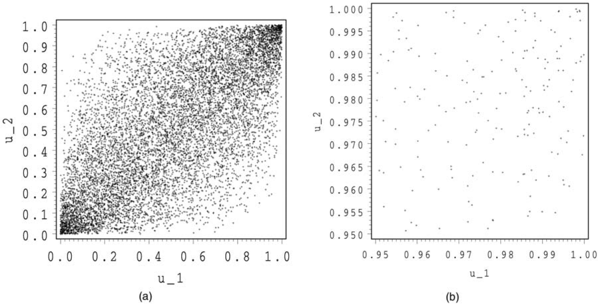
In Figures 1 and 2, we show 10,000 simulations for the normal and the Student copula. For both copulas, we make a zoom at (1,1).

Figure 1.C_0.707-copula

Figure 2.C_4,0.707-copula

We see that the Student and the normal copula have a rather similar shape. For the Student copula, there are some points around (1,0) and (0,1), whereas for the normal copula, these regions are almost empty. In the zooms, we observe a stronger concentration of points around (1,1) for the Student than for the normal copula. This illustrates the tail dependence.

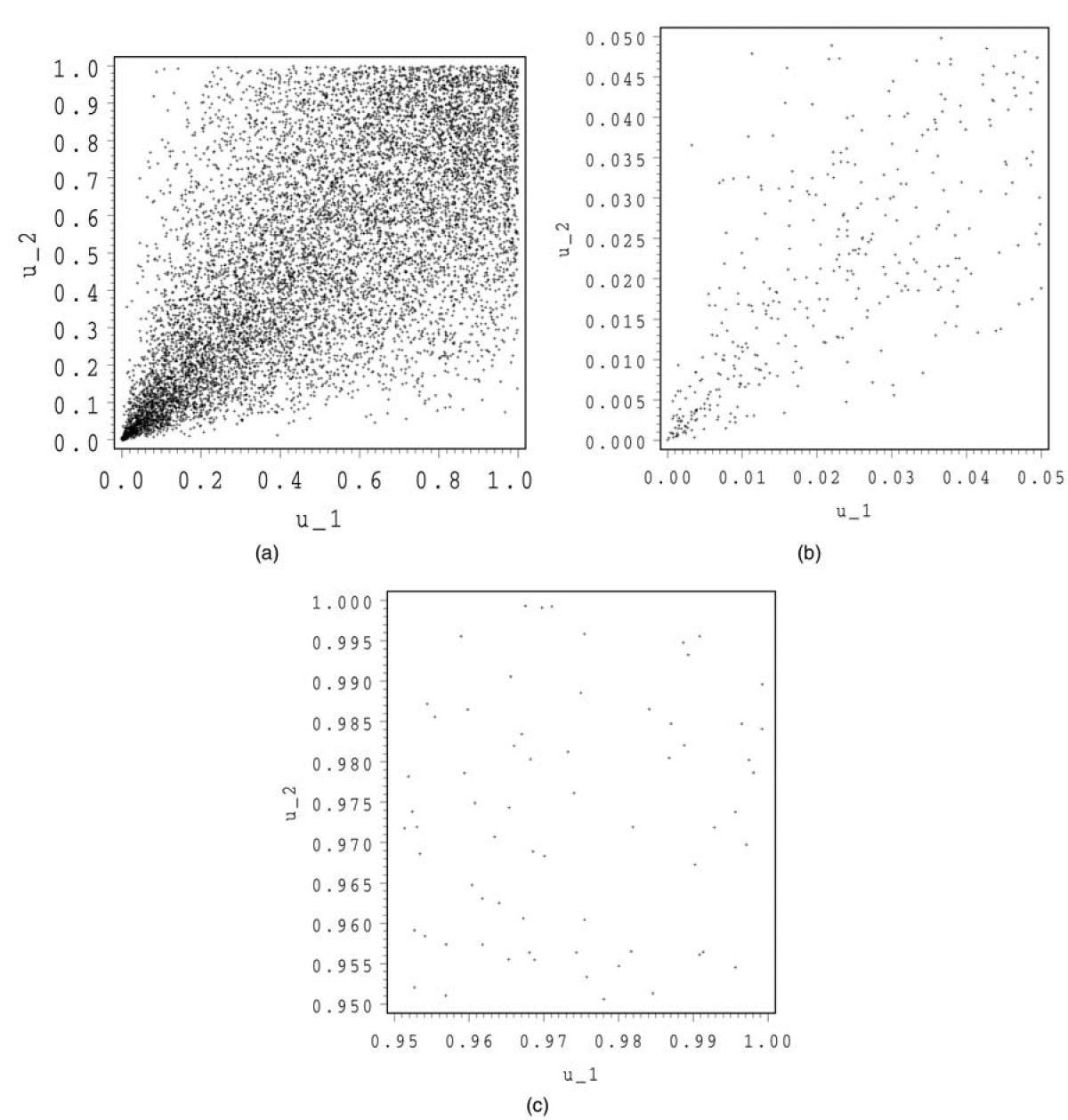
In Figure 3, we show 10,000 simulations for a Clayton copula. We make a zoom both around (0,0) and (1,1).

Figure 3.C_C,2-copula

The shape of this copula is totally different than the normal and the Student copula. In the tails, we detect a totally different behavior. The zoom at (1,1) looks more or less like an independent copula, whereas the zoom at (0,0) exhibits some kind of conic shape with a strong concentration around the origin.

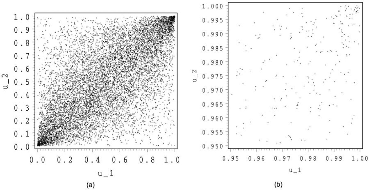
In Figures 4 and 5, we show 10,000 simulations for a Frank and a Gumbel-Hougaard copula. For both copulas, we make a zoom around (1,1).

Figure 4.C_F,5.736-copula

Figure 5.C_G,2-copula

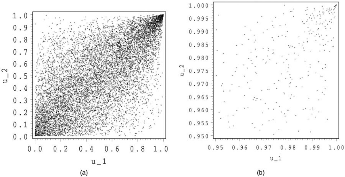
In Figure 4, we detect the symmetry for the Frank copula. The shape, however, is very different from that of the normal and the Student copula. Above the first bisector, the normal and Student copula seem to exhibit a concave shape, whereas that of the Frank copula looks more convex. The zoom of the Frank copula around (1,1) again looks like the independent copula, whereas the zoom for the Gumbel-Hougaard copula shows a concentration around (1,1).

5. Analysis of residual risk using TVaR

For every analysis we make in this section, we assume that all margins are identical. This allows comparisons between 2- and 5-dimensional results and creates some symmetry which makes interpretation more straightforward. A similar analysis can of course be made if margins are different. We look at exponential and lognormal margins. The results for exponential margins will verify the accuracy of the simulations with the results obtained in Section 2. X has a lognormal distribution with parameters μ and σ² (σ > 0) if it has the probability density function as specified by (5.1):

\[ f_{X}(x)=\frac{1}{x \sigma \sqrt{2 \pi}} e^{-(\ln (x)-\mu)^{2} / 2 \sigma^{2}} \quad \text { for all } \quad x>0 . \tag{5.1} \]

It is well known that if X ~ LN(µ,σ²),

\[ \mathbb{E}[X]=e^{\mu+\sigma^{2} / 2} \quad \text { and } \tag{5.2} \]

\[ \operatorname{Var}[X]=e^{2 \mu+2 \sigma^{2}}-e^{2 \mu+\sigma^{2}} \tag{5.3} \]

In order to work with margins that are comparable, we will fix their mean and variance. It follows easily from (5.2) and (5.3) that in order to have a lognormal distribution with mean and variance 1/λ, we need the following parameters:

\[ \begin{array}{l} \mu=-\frac{1}{2} \ln \left(2 \lambda^{2}\right) \quad \text { and } \\ \sigma=\sqrt{\ln \left(2 \lambda^{2}\right)-2 \ln (\lambda)} \end{array} \tag{5.4} \]

The same analysis can of course be made for all kinds of margins which can be simulated.

5.1. Merger of two identical companies

In Table 5, we give summary statistics for the residual risk for the merger and for the sum of the separate subsidiaries for exponential margins with parameter λ = 1/50. The results are based on 1,000,000 simulations. In order to make the results comparable, the parameters of the copulas are chosen to obtain a Kendall’s tau of 0.5, except for the comonotonic, countermonotonic, and independent copula, of course. The subscripts .95 and .99 in Table 5 indicate the level of the TVaR. The columns ℙ_.95 and ℙ_.99 give the estimated probabilities that the residual risk is 0 when a TVaR at level 0.95 or 0.99 is used as a solvency level. The numerical accuracy of the results in the independent case can be compared with Table 1. Except for the comonotonic case, the simulations for the margins are not necessarily the same. The comparison of the results for the mean residual risk and the sum of the TVaRs for the separate subsidiaries gives an idea about their numerical variability.

In Table 5, we observe that among all dependence structures, there is a maximum diversification benefit on the TVaR for the merger of about 41% on the 0.95-level and 44% on the 0.99-level in the countermonotonic case. When we compare the normal and the Student copula, we observe that the Student copula requires more capital due to the tail dependence, but it should be noted that the difference, certainly at a 0.95-level, is small. The difference is larger if the solvency level increases. For a higher probability level, we detect a smaller difference between the average residual risk for the merger and the standalones for the Student copula, whereas for the normal copula it is nearly constant. We also see a clear influence of the strong tail dependence for the flipped Clayton and the Gumbel-Hougaard copula. There is almost no diversification effect in such an environment. Increasing the solvency level makes the effect on the capital even smaller. This is opposed to the situation for the Frank, the Clayton, and to a lower extent also for the flipped Gumbel-Hougaard copula. These copulas exhibit a clear diversification benefit both on the capital requirement and on the mean of the residual risk, which increases with the solvency level. We observe that when looking at capital requirements, it is very important to correctly take into account the stochastic dependence in the tails. Our simulations illustrate that if strong tail dependence is present but is not taken into account, the required capital can be substantially underestimated. With respect to the standard deviation of the residual risk, we note for most of the cases with a Kendall’s tau of 0.5 an increase for the merger. Only for the Clayton and the Frank copula does this statistic decrease. Note that the level of dependence we chose may be fairly high for practical considerations. Still, the increase when compared to the standalone scenario is never larger than 10%. The probability of default can be substantially decreased by merging the risks, mainly in situations where tail dependence is low.

In Table 7, we give the same results as in Table 5 but now for two identical lognormal margins with mean and standard deviation equal to 50 and for a Kendall’s tau of 0.25. It follows from (5.4) that the margins have parameters µ = 3.565 and σ = 0.8326. The choice for Kendall’s tau implies that the copulas have parameters and tail dependence as specified in Table 6.

In Table 6, we see that the lower tail dependence for the Clayton copula is, just as for a Kendall’s tau of 0.5, larger than the upper tail dependence for the Gumbel-Hougaard and the tail dependence for Student copula.

In Table 7, we observe that among all dependence structures, there is a maximum diversification benefit on the TVaR for the merger of about 36% on the 0.95-level and 40% on the 0.99-level. If we exclude the comonotonic case, we again have a minimum diversification benefit for the flipped Clayton copula, which is about 9% both at a 0.95 and 0.99 probability level. For the Gumbel-Hougaard copula, the diversification benefit on the TVaR now also remains nearly constant in function of the probability level, whereas for the Student copula, it now even increases with the probability level. However, for each of the latter three copulas, the average residual risk still shows a lower relative diversification benefit when increasing the probability level. We see a clear influence of the fatter tails for the lognormal marginals both on the TVaR and on the risk measures of the residual risk. The subadditivity of the TVaR is never such that it increases the average residual risk of the merger. However, in cases with (strong) positive tail dependence, the diversification benefit on the residual risk remains small if we compare with the independent situation and with the situations without tail dependence. The probabilities of default are slightly larger than for the exponential margins, which have less fat tails.

5.2. Merger of five identical companies

In Table 8, we give the results of the same simulations as in Table 5 but in five dimensions. Note that for the normal and the Student copula, all elements in the correlation matrix, apart from those on the diagonal, are equal to the value specified in Table 4. This may in practice, of course, not be very realistic, but we make this choice in order to use copulas which are comparable with respect to their Kendall’s tau. It is clear that for the normal and Student copulas, it is possible to use different dependence structures between the margins (if we look at them 2 by 2), whereas for multivariate Archimedean copulas, the dependence structure between the margins (2 by 2) is always the same and based on solely one parameter.

As we could expect, the diversification benefit on the TVaR and the default probability is now always larger than in the two-dimensional situation. For the average residual risk, we have a higher diversification benefit as well. From our list of copulas, the independent situation now leads to the highest diversification benefit. For the rest, the same conclusions hold as in two dimensions. In cases where the volatility of the residual risk of the merger increased compared to the standalone situation, it now increases more and vice versa if it decreased. If our main interest is the average residual risk or the default probability, in these examples, the TVaR is never too subadditive.

In Table 9, we give the same results as in Table 7 but for five identical lognormal risks.

In the case the risks are independent, we again observe a very substantial benefit on the required capital. For all copulas, the relative decrease of the TVaR and of the average residual risk is again more important than when we compare with the two-dimensional case. Just as we observed by comparing Table 5 and 8, if in two dimensions, the standard deviation of the residual risk of the merger increased compared to that of the sum of the standalone companies, it now increases more and vice versa if it decreased.

In Table 10, we give the same results as in Table 9 but for five identical lognormal risks with mean 50 and a coefficient of variation (COV) of 25%. This means that we use the parameters µ = 3.882 and σ = 0.2462 for the margins. This may correspond better to the shape of aggregate distributions for different lines of business.

In this setting, the tail is substantially smaller than for a COV of 100%. Therefore, the TVaR is reduced importantly. The relative diversification benefit on the TVaR for the merger varies between 52% of the value in Table 9 for the independent copula and 38% for the Gumbel copula (both at a 99% level). At a 95% level, the relative diversification benefit on the average residual risk for the mergers is reduced most importantly for the Gumbel and the flipped Clayton copula (resp. 4% and 26% of the diversification benefit in Table 9). For the other copulas, it varies between 63% of the level in Table 9 for the Student copula and 93% of this level for the independent copula. A comparable conclusion can be drawn at a 99% level. For all simulations, the diversification “benefit” on the standard deviation of the residual risk is lower than in Table 9. The probabilities that the residual risk is zero are slightly lower than in Table 9. The differences between the default probabilities for the merger and the standalones increase about 10% in these scenarios.

In all five-dimensional examples, the TVaR seems to give an acceptable benefit to the diversification for the merger. The subadditivity of the TVaR is never such that the average residual risk and the probability of default of the merger increase compared to the situation of the standalones.

6. Conclusion

Our examples have clearly demonstrated the possible diversification benefit when risks are being merged. This benefit plays not only on the required capital but also on the residual risk after capital allocation and on the default probability. If the TVaR is used as a risk measure, merging risks can be in the interest both of the shareholders and of the regulator defending the interests of the policyholders. When using the average residual risk as a benchmark, our examples demonstrate that the TVaR is not too subadditive under a wide range of dependence structures. The same holds when the default probability is considered. The standard deviation of the residual risk for the merger can be both larger and smaller than the standard deviation of the sum of the residual risk for the standalone companies, depending on the strength of the (tail) dependence. These results make us believe that the TVaR is a very valid candidate for a risk measure providing, in itself, a basis for compromise between the interests of the shareholders and the regulator.

Based on a simulation model taking various copulas for describing the dependence structure between the margins, we have seen that results for copulas which all have the same Kendall’s tau may be very different. This clearly illustrates the importance of the tails in general and the effect of tail dependence in particular for capital calculation purposes. If possible tail dependence in the data is being neglected, this may lead to a capital relief for a merger which is too large.

In case of positive upper tail dependence and a high value for Kendall’s tau, the diversification benefit on the capital relatively decreases if we increase the solvency level. If Kendall’s tau and the strength of the upper tail dependence decrease, this is not necessarily true. When there is no upper tail dependence, a higher solvency level leads to a higher relative diversification benefit, both for higher and lower values for Kendall’s tau.

In a multidimensional setting, Archimedean copulas based on one parameter may lack flexibility to effectively capture the dependence structure. The normal and Student copulas are more flexible in this sense, since they allow the user to work with more parameters based on a correlation matrix. The normal copula has the drawback that is does not allow the user to model tail dependence. We have seen that the tail dependence for the Student copula drives the results for the normal and Student copula further apart for higher probability levels. Further analysis based on real-life data should be made to see whether the Student copula is flexible enough to capture the tail dependence in an appropriate manner.

Acknowledgments

The authors are grateful to the review team for valuable comments that have led to a better presentation of the paper.