


1. The essence
In the usual collective risk model, actuaries ask how many events there are in a time period. This is followed by asking how big each event is. In a timeline formulation, we ask how long it is until the next event, followed by how big the event will be. This change of focus is the subject of this paper.[1]
With a timeline formulation the emphasis is on the instantaneous frequency—the propensity to generate a claim of some type at any point in time. The number of claims in a time period emerges as a counting exercise. This is a mathematically equivalent formulation for all the commonly used distributions. Furthermore, the notion of frequency, rather than count, is what claims people and actuaries are really thinking about. A statement like “the frequency of fender-benders goes up in the winter” is intuitively clear and goes to the heart of the matter, whereas “the number of fender-benders in a specified time period smaller than a season goes up in the winter” just sounds awkward.
Why have actuaries used collective risk models? Some contributing factors are that the data we see is arranged by period, such as accident year or quarter; that we can calculate interesting properties such as the moments of the aggregate distribution; that the implicit assumption of the independence of frequency and severity is empirically often acceptable; and that the available computing power limits the calculation.
The next section will discuss the general properties of a timeline formulation; Section 3 is dedicated to theory and may be skipped on first reading; Section 4 describes the operational practice of doing simulations; and Section 5 has examples taken from the companion spreadsheet.
2. Consequences of and motivation for a timeline formulation
Most obviously, a timeline formulation is more real than collective risk because events in the real world actually do happen at points in time and in a definite order. Typical events under consideration might be the occurrence of a claim, payments on a claim, reinsurance recoveries and premiums, and so on. In any type of simulation model, there are a number of random variables. By a realization we mean that each of the relevant variables has taken on a value, yielding a numerical result. A large number of realizations together, often referred to as a simulation set, gives information about the probabilities of various results. In a collective risk model, a realization typically proceeds by first generating some number of events and then generating severities. Contrary to a timeline model, there is no notion of when or in what order the events occur. In reinsurance work a contract can cover several lines of business and have an aggregate limit. If all the claims from line A are applied first and exhaust the limit, then the model will suggest that line A really gets all the ceded losses. In order to avoid this, models will randomize the order of application of losses to the contract to get a better feel for which lines really get what share of the losses. If line B is seasonal and line A is not, then the randomization needs to take this into account. In fact, what is needed is to assign a time-appropriate order of occurrence. At least one model does this internally, but does not report it out. In a timeline formulation, seasonality, trend, and calendar year influences have a natural implementation.
A related property is that the results on a timeline are perfectly transparent. You can look at any individual realization and see exactly which claims hit which contracts in what order and see how the contracts responded, depending on what happened before. For example, you can see what caused an aggregate limit to be filled and a backup contract to be invoked. Any individual realization is easy to understand because all the information is explicitly available in an intuitive form.
Further, since events are often influenced by prior events, truly causal relationships can be modeled explicitly. Exposure as a random variable can simultaneously drive the frequency of large losses in a line, the severity of bulk[2] losses, and the written premium. A change in inflation can affect auto parts prices; a change in the unemployment rate can affect workers compensation claims, and so on. Discounting, even with time varying discount rates, can be done on an individual payment basis. Since we are working one event at a time, we can ask for all of the influences on the event’s instantaneous frequency and severity. The whole prior history is available for each event. The challenge becomes deciding what to model and then actually modeling the effects.
Since we are working with instantaneous frequency, we do not need to assume that frequency and severity are independent, provided we have some sensible model that connects them, such as a quantification of “successful large claims engender more of the same.” The success of a new theory of liability (think toxic mold) can produce this, as can a changing court climate.
Also, the generation of simulated events is separated from the reporting on events. In a collective risk model, a change in the reporting interval requires a change in the frequency parameterizations. In a timeline formulation there are no parameter changes, and going from annual to quarterly reporting looks at the same events on a timeline and only changes the relevant time intervals. Accident year, report year, and policy year reports are just summaries of different subsets of the same events on a timeline, so consistency is automatic.
Management decision rules based on periodic or even instantaneous reports can be implemented. If we can state the decision rules, then we can model their effects. For example, “cut writings in line A by 20% if the midyear claim count is 75% of last year’s total” gives a complete-enough algorithm to implement in a timeline formulation. Or, “We just had four hurricanes this year in Florida. Let’s get out of there.”
Whereas a timeline formulation allows any collective risk model to be implemented, it also allows many kinds of calculations to be done exactly rather than by hopeful approximation. For example, collective risk model formulations will often assume that everything happens in midyear, and inflation and discounting are taken at those values. Not everything actually does happen at midyear. On the other hand, the European index clause in its various forms actually requires indexation by a possibly random index at the random times of occurrence and payment(s). This can easily be done in a timeline formulation. Approximations must also be made if there are a variable number of multiple payments, or their number or amount is not determined at the time of occurrence, or there is an exotic pattern such as a number of small ALAE payments whether followed by a big loss or not.
Perhaps most importantly, a timeline formulation encourages a different way of thinking that leads to new kinds of simple models. For example, it is often said that larger claims usually close later than smaller claims. The intuition is that large claims are more worth defending in court than small claims. In a collective risk model, you would have to have separate payout patterns by claim size, with a great many parameters. In a timeline formulation, one possible simple model would generate a loss size, and then a time to payment with the mean time proportional to the size of loss.[3] This example illustrates the ease of creating a simple model which generates count and dollar triangles that can be compared to data. In fact, claims departments have the actual dates—occurrence and payment—that could be used to create and validate (or invalidate) models. We actuaries have just never looked at the data that way, because we always have worked with aggregated data.
Conversely, there are many claims that sit at small values for a long time and then become very large just before closing. Perhaps a simple model would have the mean severity depend nonlinearly on the time to closure. A reinsurance cancellation on treaties with seasonal effects can and probably should be done pro rata on exposure (via the frequency changes) rather than on time.[4] Finally, a new graduation technique for payment patterns from accident period data has emerged,[5] creating a continuous payment distribution of time from occurrence.
3. Theory
The reader who wants to know immediately how all this works in practice and to work with the spreadsheet is encouraged to skip this section, perhaps for later perusal. The two most salient facts are that a Poisson process is a constant instantaneous frequency, and that a negative binomial is a gamma-mixed instantaneous frequency.
The formulation is done in terms of continuous time, and the derivations in this section have no doubt appeared in various works of probability and statistics.[6] The author has tried to keep everything self-contained here so that no outside references are needed. The calculus is minimal, but the fundamental relation for probabilities is a first-order differential equation. Those for whom calculus is a long time ago, in a galaxy far far away, may wish to just trust the derivations and use the results. Section 4 gives the algorithms actually used, and the theoretical framework is only intended to justify the algorithms and give some sense for the notion of instantaneous frequency. Although the framework and algorithms are simple, because of the housekeeping involved, the implementation in code is tedious but straightforward.
We begin with a definition of instantaneous frequency and a derivation of the general time-dependent probability equation, followed by Poisson and negative binomial examples. In the second part of this section we address the question of mixing distributions, revisiting the negative binomial and introducing a new distribution. If for no reason other than parameter uncertainty, we must be able to handle mixing distributions. They arise naturally when one draws from the parameter distributions to get frequencies. Details of much of the proofs are left to appendices.
3.1. Instantaneous frequency
The underlying assumption is that in an arbitrarily short time interval △t, there can be at most one[7] event and the probability of it happening is proportional to the size of the time interval. The proportionality “constant” is the instantaneous frequency. This is the definition of the instantaneous frequency, as probability per time[8] over a very short time interval:
\[ \operatorname{Pr}=\lambda(t, n, \ldots) \Delta t . \tag{3.1} \]
The quantity λ is the instantaneous frequency, which may depend on the time t, the number n of events already present, exogenous influences such as economic indices or legal climates, or anything else in the past history. Intuitively, the instantaneous frequency is the propensity for an event to happen. In what follows, we generally will only show the first two arguments of λ. The essential requirement that probabilities be non-negative means that the instantaneous frequency is never negative. Generally speaking, we will work with simple forms for the instantaneous frequency, but some results do not depend on the explicit form and we will not restrict it until we consider the Poisson case in Section 3.4.
We will now state the basic relationship for probabilities at a small △t and then get a first order differential equation by going to the limit △t → 0. In order to have n events at t + △t you either have n at t and do not get another, or you have n − 1 and a new one occurs. Thus, the probability of having exactly n events at time t + △t is the sum of the probability of n events at time t times the probability of no events between t and t + △t plus the probability of n − 1 events at time t times the probability of one event between t and t + △t.
With Pn(t) being the probability of exactly n events at time t, the probability statement becomes
\[ \begin{aligned} P_{n}(t+\Delta t)= & P_{n}(t)[1-\lambda(t, n) \Delta t] \\ & +P_{n-1}(t)[\lambda(t, n-1) \Delta t] \end{aligned} \tag{3.2} \]
The boundary condition at time t = 0 is that there are no events:[9] P0(0) = 1, Pn(0) = 0 for all n > 0. Rearranging Equation (3.2) we have
\[ \begin{aligned} \frac{P_{n}(t+\Delta t)-P_{n}(t)}{\Delta t}= & -\lambda(t, n) P_{n}(t) \\ & +\lambda(t, n-1) P_{n-1}(t) \end{aligned} \tag{3.3} \]
and taking the limit as △t → 0 we get the fundamental relationship in the form of a first-order differential equation
\[ P_{n}^{\prime}(t) \equiv \frac{d}{d t} P_{n}(t)=-\lambda(t, n) P_{n}(t)+\lambda(t, n-1) P_{n-1}(t) \tag{3.4} \]
We have introduced the convenient “prime” notation P′n(t) ≡ (d/dt)Pn(t) for a derivative with respect to time, since it will occur so often.
In the particular case n = 0 there is no second term on the right of Equation (3.4), and we have
\[ P_{0}^{\prime}(t)=-\lambda(t, 0) P_{0}(t) \tag{3.5} \]
The solution[10] satisfying the boundary condition at time zero P0(0) = 1 is
\[ P_{0}(t)=\exp \left\{-\int_{0}^{t} \lambda(\tau, 0) d \tau\right\} \tag{3.6} \]
since
\[ \begin{aligned} \frac{d}{d t} P_{0}(t) & =P_{0}(t) \frac{d}{d t}\left\{-\int_{0}^{t} \lambda(\tau, 0) d \tau\right\} \\ & =-\lambda(t, 0) P_{0}(t) \end{aligned} \tag{3.7} \]
and
\[ P_{0}(0)=\exp \left\{-\int_{0}^{0} \lambda(\tau, 0) d \tau\right\}=\exp \{0\}=1 \tag{3.8} \]
3.2. Waiting time
Now that we have the time probability of zero events, we may talk about waiting times—the times between events. The cumulative distribution of waiting time for the first event is the probability that we no longer have zero events:
\[ F(T)=1-P_{0}(T)=1-\exp \left\{-\int_{0}^{T} \lambda(\tau, 0) d \tau\right\} \tag{3.9} \]
The probability density for the distribution of waiting time is its derivative
\[ f(T)=F^{\prime}(T)=\lambda(T, 0) \exp \left\{-\int_{0}^{T} \lambda(\tau, 0) d \tau\right\} \tag{3.10} \]
The extensions to the case of waiting time to the next event where there are already n events at time t are
\[ F(T)=1-\exp \left\{-\int_{t}^{T} \lambda(\tau, n) d \tau\right\} \tag{3.11} \]
and
\[ f(T)=\lambda(T, n) \exp \left\{-\int_{t}^{T} \lambda(\tau, n) d \tau\right\} . \tag{3.12} \]
In practice, one would look at the data and fit a parameterized form to λ by a method such as maximum likelihood. We are already accustomed to doing this for severities, so it is not a new process. In the discussion of parameter estimation in Appendix B, Equation (B.9) provides a generalization of Equation (3.12) in the presence of mixing distributions.
The mean waiting time for the first event is
\[ \begin{aligned} E(T) & =\int_{0}^{\infty} T f(T) d T \\ & =\int_{0}^{\infty} T \lambda(T, 0) \exp \left\{-\int_{0}^{T} \lambda(\tau, 0) d \tau\right\} d T \end{aligned} \tag{3.13} \]
In the important special case of constant instantaneous frequency (i.e., Poisson), the mean waiting time for the first event is
\[ E(T)=\int_{0}^{\infty} T \lambda e^{-\lambda T} d T=1 / \lambda \tag{3.14} \]
3.3. Time dependence of the mean
Returning to the fundamental relation Equation (3.14), an immediate consequence is the evaluation of the time rate of change of the mean number of events. The mean number of events at any time is
\[ \text { mean }(t)=\sum_{n=0}^{\infty} n P_{n}(t) \tag{3.15} \]
Its time rate of change is, using Equation (3.4),
\[ \begin{aligned} \frac{d}{d t} \operatorname{mean}(t) & =\sum_{n=0}^{\infty} n P_{n}^{\prime}(t) \\ & =\sum_{n=0}^{\infty} n\left[-\lambda(t, n) P_{n}(t)+\lambda(t, n-1) P_{n-1}(t)\right] \\ & =\sum_{n=0}^{\infty}\left[-n \lambda(t, n) P_{n}(t)+(n+1) \lambda(t, n) P_{n}(t)\right] \\ & =\sum_{n=0}^{\infty} \lambda(t, n) P_{n}(t) \end{aligned} \tag{3.16} \]
This has the natural interpretation that the rate of change of the mean at any time is the probability weighted average over the instantaneous frequency at different counts. In a case where the instantaneous frequency does not depend on the number of events, the probabilities sum to 1 and Equation (3.16) becomes
\[ \lambda(t)=\frac{d}{d t} \text { mean }(t) \tag{3.17} \]
Here, the instantaneous frequency is the rate of change of the mean, which perhaps gives another intuitive handle for thinking about the instantaneous frequency.
3.4. Poisson process
What defines a Poisson process is that the instantaneous frequency λ is constant. This means that there is no memory of past history, and the probabilities of events in any time interval are the same as in any other time interval of equal size. Equation (3.17) implies that the mean number of events in a time interval is the interval size multiplied by λ.
Let us solve Equation (3.4) for this case.[11] We will take up another case later, where the λ depends linearly on the number of claims. For the Poisson, Equation (3.4) becomes
\[ P_{n}^{\prime}(t)=-\lambda\left[P_{n}(t)-P_{n-1}(t)\right] . \tag{3.18} \]
The solution is derived in Appendix A, and is the familiar
\[ P_{n}(t)=\frac{(\lambda t)^{n}}{\Gamma(n+1)} e^{-\lambda t} . \tag{3.19} \]
In timeline formulation, a Poisson is the simplest possible random generator of events.
The Poisson provides a very important special case of Equation (3.9), which then says that the cumulative distribution of waiting time from time t is
\[ F(T)=1-e^{-\lambda(T-t)} \tag{3.20} \]
That is to say, the waiting times are exponentially distributed. We can simulate the interval to the next event by
\[ T-t=-\frac{1}{\lambda} \ln (\text { uniform random }) . \tag{3.21} \]
In the algorithms for the next section, it is this result that is used to find the time for the next event.
In fitting to sample data, the solution for λ is one divided by the sample average waiting time and the uncertainty in λ is λ divided by the square root of the number of observations for a flat Bayesian prior. We will return to this in Appendix B, but for now note that the number of observations is the number of claims minus one and not the number of years, yielding a potentially much better determination of the parameter.
3.5. Count-dependent frequency
Another case of interest because of its relation to other well-known counting distributions has the instantaneous frequency linear in the count:
\[ \lambda(t, n)=\lambda+b n . \tag{3.22} \]
Since the instantaneous frequency must be positive, we will consider for the moment the case b > 0. It is obvious that in the limit b → 0 we must recover the Poisson case. Putting this form into the Equation (3.16) for the derivative of the mean, we get
\[ \begin{aligned} \frac{d}{d t} \text { mean } & =\sum_{n=0}^{\infty} \lambda(t, n) P_{n}(t) \\ & =\sum_{n=0}^{\infty}(\lambda+b n) P_{n}(t)=\lambda+b \text { mean. } \end{aligned} \tag{3.23} \]
The solution for this which is zero at time zero is
\[ \text { mean }=\frac{\lambda}{b}\left(e^{b t}-1\right) . \tag{3.24} \]
We note that as b → 0 the mean goes to λt, as it should. The salient feature is that the mean is exponentially growing with time—not particularly a surprise given that we have made the rate of increase of the mean proportional to the number of claims. This is the standard population growth with unlimited resources.
What is perhaps more surprising is that the distribution at any fixed time is negative binomial. The solution[12] of the fundamental Equation (3.4) with the frequency given by Equation (3.22) is
\[ P_{n}(t)=\frac{\left(1-e^{-b t}\right)^{n} e^{-\lambda t} \Gamma(\alpha+n)}{\Gamma(n+1) \Gamma(\alpha)}, \tag{3.25} \]
where we have defined α ≡ λ/b. A negative binomial distribution with parameters[13] ρ and α has count probabilities given by
\[ P_{n}=\frac{\rho^{n}(1-\rho)^{\alpha} \Gamma(\alpha+n)}{\Gamma(n+1) \Gamma(\alpha)} . \tag{3.26} \]
We can see that Equation (3.25) is Equation (3.26) when we identify ρ = 1 − e−bt and hence (1 − ρ)α = e−αbt = e−λt.
As an aside, if we allow b < 0 and set λ(t, n) = max(λ + bn, 0), then when α ≡ λ/b = −N is a negative integer, at any fixed time we have a binomial distribution whose mean is N(1 − e−λt/N).
3.6. Mixing distributions
We are forced to consider mixtures of Poisson distributions when we think about even the most limited form of parameter uncertainty, the uncertainty resulting from limited data. See Appendix B, Equation (B.5) for an example in the simple case. We may also be led there by our intuitions about the actual underlying process. We may think of it either as a probabilistic mix of Poisson processes, say a random choice between two values, or we may think of it as reflecting our uncertainty about the true state of the world. The algorithms in the next section presume that any individual realization is basically Poisson with one or more sources, but with parameters that vary from realization to realization (or even within one realization) so that the resulting count distributions may be extremely complex. In simulation, we will begin each realization by choosing a state of the world based on a random draw from the parameter distributions. For Poisson sources, this amounts to using a mixed Poisson.
In the general case, we assume a given probability density on λ. Let f(λ) be the density for the mixing distribution. Then the probability of seeing n events at time t is the probability of seeing n events given λ [Equation (3.19)] times the probability of that value of λ, summed over all λ:
\[ P_{n}(t)=\int_{0}^{\infty} \frac{(\lambda t)^{n} e^{-\lambda t}}{\Gamma(n+1)} f(\lambda) d \lambda \tag{3.27} \]
We may express the moments of the count distribution in terms of the moments of the mixing distribution using Equation (A.7):
\[ \begin{array}{l} E(n(n-1)(n-2) \ldots(n-K+1)) \\ \quad \equiv \sum_{n=0}^{\infty} n(n-1)(n-2) \ldots(n-K+1) P_{n} \\ \quad=t^{K} \int_{0}^{\infty} \lambda^{K} f(\lambda) d \lambda \end{array} \tag{3.28} \]
Specifically, the mean is given by the mean of the mixing distribution multiplied by the time:
\[ E(n)=t \int_{0}^{\infty} \lambda f(\lambda) d \lambda \equiv \mu t \tag{3.29} \]
The variance to mean ratio is that of the mixing distribution multiplied by the time plus one, as shown by
\[ \begin{aligned} \operatorname{var}(n) & \equiv \sum_{0}^{\infty} n^{2} P_{n}-(\mu t)^{2}=\sum_{0}^{\infty} n(n-1) P_{n}+\mu t-\mu^{2} t^{2} \\ & =t^{2}\left[\int_{0}^{\infty} \lambda^{2} f(\lambda) d \lambda-\mu^{2}\right]+\mu t=t^{2} \operatorname{var}(\lambda)+\mu t \end{aligned} \tag{3.30} \]
so that
\[ [\mathrm{var} / \text { mean }]_{\text {count }}=1+t[\mathrm{var} / \text { mean }]_{\text {mixing }} . \tag{3.31} \]
The simple Poisson thus has the smallest possible variance to mean ratio. The skewness (and all higher moments) of the count distribution can be similarly derived from those of the mixing distribution, but generally do not have an orderly form.
3.7. The simplest mix—Two Poissons
For the mixture, we take the instantaneous frequency to be λ1 with probability p and λ2 with probability 1 − p. Formally, the density function in λ is[14]
\[ f(\lambda)=p \delta\left(\lambda-\lambda_{1}\right)+(1-p) \delta\left(\lambda-\lambda_{2}\right) . \tag{3.32} \]
The count distribution from the definition Equation (3.27) is then
\[ P_{n}(t)=\frac{t^{n}}{\Gamma(n+1)}\left[p \lambda_{1}^{n} e^{-\lambda_{1} t}+(1-p) \lambda_{2}^{n} e^{-\lambda_{2} t}\right] . \tag{3.33} \]
The mean of this mixing distribution (and by Equation (3.29) the mean of the count distribution at time t = 1) is the intuitive result
\[ \begin{aligned} E(\lambda) & =\int_{0}^{\infty} \lambda f(\lambda) d \lambda \\ & =\int_{0}^{\infty} \lambda\left[p \delta\left(\lambda-\lambda_{1}\right)+(1-p) \delta\left(\lambda-\lambda_{2}\right)\right] d \lambda \\ & =p \lambda_{1}+(1-p) \lambda_{2} \end{aligned} \tag{3.34} \]
The second moment similarly is
\[ \begin{aligned} E\left(\lambda^{2}\right) & =\int_{0}^{\infty} \lambda^{2} f(\lambda) d \lambda \\ & =\int_{0}^{\infty} \lambda^{2}\left[p \delta\left(\lambda-\lambda_{1}\right)+(1-p) \delta\left(\lambda-\lambda_{2}\right)\right] d \lambda \\ & =p \lambda_{1}^{2}+(1-p) \lambda_{2}^{2} \end{aligned} \tag{3.35} \]
so the variance is
\[ \operatorname{var}(\lambda)=E\left(\lambda^{2}\right)-E(\lambda)^{2}=p(1-p)\left(\lambda_{1}-\lambda_{2}\right)^{2} . \tag{3.36} \]
And the variance to mean of the count distribution is, by Equation (3.31)
\[ [\mathrm{var} / \text { mean }]_{\text {count }}=1+t \frac{p(1-p)\left(\lambda_{1}-\lambda_{2}\right)^{2}}{p \lambda_{1}+(1-p) \lambda_{2}} . \tag{3.37} \]
3.8. Negative binomial as gamma mix
This is an important special case, because of the frequent use in actuarial work of the negative binomial distribution. The intuition is that the frequencies are spread in a unimodal smooth curve from zero to infinity. One simple form uses a gamma mixing distribution:
\[ f(\lambda)=\frac{\lambda^{\alpha-1} e^{-\lambda / \theta}}{\theta^{\alpha} \Gamma(\alpha)} \tag{3.38} \]
In terms of these parameters, the mean is αθ and the variance to mean is θ. Using Equation (3.27) the count distribution is
\[ \begin{aligned} P_{n}(t) & =\int_{0}^{\infty} \frac{(\lambda t)^{n} e^{-\lambda t}}{\Gamma(n+1)} \frac{\lambda^{\alpha-1} e^{-\lambda / \theta}}{\theta^{\alpha} \Gamma(\alpha)} d \lambda \\ & =\frac{\left(\frac{\theta t}{1+\theta t}\right)^{n}\left(\frac{1}{1+\theta t}\right)^{\alpha} \Gamma(n+\alpha)}{\Gamma(n+1) \Gamma(\alpha)} . \end{aligned} \tag{3.39} \]
Comparing to Equation (3.26) we can see that this is negative binomial with parameter ρ = θt/(1 + θt). Then from Equations (3.29) and (3.31) or directly from the moments of the negative binomial, the mean of the count distribution is βθt and the variance to mean ratio is 1 + θt. Most of note, in contrast to the contagion case of count dependence (Section 3.5) here the negative binomial has a mean linear rather than exponential in the time.
3.9. Uniform mix
The intuition here is when the analyst says, “I think the instantaneous frequency is in this range, but not outside.” This is similar in spirit to a diffuse Bayesian prior which is limited. Like the gamma mix, it has two parameters but they are perhaps more easily interpreted, being values rather than the moments. Specifically, for a uniform mix between a and b > a the distribution is
\[ \begin{array}{l} f(\lambda)=\frac{1}{b-a} \quad \text { for } \quad a \leq \lambda \leq b\\ \text { and zero otherwise. } \end{array} \tag{3.40} \]
The mean of this distribution is (a + b)/2, and the variance to mean ratio is (b − a)2/6(a + b). The count distribution is
\[ \begin{aligned} P_{n}(t) & =\int_{a}^{b} \frac{(\lambda t)^{n} e^{-\lambda t}}{(b-a) \Gamma(n+1)} d \lambda \\ & =\frac{G(b t, n+1)-G(a t, n+1)}{(b-a) t} \end{aligned} \tag{3.41} \]
where G(λ, n) is the incomplete gamma distribution with integer parameter
\[ \begin{aligned} G(\lambda, n) & \equiv \int_{0}^{\lambda} \frac{x^{n-1} e^{-x}}{\Gamma(n)} d x \\ & =1-e^{-\lambda}\left\{1+\lambda+\frac{\lambda^{2}}{2}+\cdots+\frac{\lambda^{n-1}}{\Gamma(n)}\right\} . \end{aligned} \tag{3.42} \]
We can recognize 1 − G(λ,n + 1) as the cumulative distribution function for a Poisson with parameter λ. Intuitively this makes sense, as we are representing the count probability density as a finite difference approximation on the cumulative distribution function.
3.10. Arbitrary probabilities
We need to be able to work with any given set of count probabilities. Ideally, we would like to invert Equation (3.27) and be able to determine a mixing function for any set of probabilities. This is in fact possible, and unique, but the mixing function may not be a probability density because it is not guaranteed that f(λ) ≥ 0. Take as an obvious example a distribution with exactly one count: P1 = 1, all other probabilities are λ zero. Since 0 = P0(t) = ∫0∞ e−λtf(λ)dλ, clearly f(λ) < 0 somewhere. Nevertheless, there always is such a mixing function.
That does not mean we cannot simulate with an arbitrary set of annual count probabilities. Actually, it is rather easy. We generate a count for each year of our horizon and assign random times within the year to the events. If we have a fractional year in our horizon, we generate the annual count but only take the events inside the horizon. What we lose is any causal connection between events, but in a count distribution that is not present anyway.
It is shown in Appendix C, freely ignoring considerations of rigor, how to get a unique mixing function. The solution is framed in terms of the Laguerre polynomials of parameter zero, defined as
\[ L_{n}(x) \equiv \frac{e^{x}}{\Gamma(n+1)} \frac{d^{n}}{d x^{n}}\left(e^{-x} x^{n}\right) . \tag{3.43} \]
They are used because they are orthogonal with weight e−x. Create the auxiliary quantities
\[ Q_{n} \equiv \sum_{k=0}^{n} \Gamma(k+1) d_{k}^{n} P_{k} \tag{3.44} \]
with dkn being the coefficient of xk in the Laguerre polynomial of order n and Pk being the desired probabilities. The mixing function can be expressed as
\[ f(\lambda)=\sum_{n=0}^{\infty} Q_{n} L_{n}(\lambda) \tag{3.45} \]
Using this mixing function in Equation (3.27) will give back the probabilities Pn.
4. Practice
In this section we will discuss the implementation of timeline simulation. In the next, we will refer to various examples and their implementation in the companion spreadsheet. The examples will illustrate the principles given here, as well as leading the reader through one particular implementation of the timeline formulation. Readers are encouraged to build their own simulation platform, because reading about it and trying to understand someone else’s complex workbook will not give the same depth of understanding. Therefore, experimentation with the spreadsheet is strongly encouraged.
4.1. Basics of timeline simulation
The fundamental paradigm is that events occur on a time line, changing the state of the world. Events can be randomly generated, scheduled, or arise in response to other events. This final property leads to event cascades. Time runs to a prespecified horizon, and then reports (possibly including known future events) are made on the events on the timeline. Reports can also be made on a periodic or even instantaneous basis. They can also be generated in response to a particular event or series of events.
An event is essentially anything of interest at a particular time. For most dynamic risk model analyses, prototypical events would be cash flow amounts at particular times with tags indicating the type of accounting entry, the line of business, perhaps the location, and anything else of relevance. Exogenous variables such as consumer price index values can also be events of interest.
Fundamentally, what defines “of interest” is the kinds of reports that are desired, and these are determined by the kinds of questions the analysis is designed to answer. Most frequently, these questions are couched in financial terms, and often in terms of impact on an insurance company financial statement. Income statements are sums of dollars and counts of events during specified time intervals, identified by accounting entry type and line of business. Sometimes in order to generate an event of interest, say a reinsurance cession, other informative events will be required, such as exterior index values, which then become of interest.
Some examples of possible event generators are losses (catastrophe, non-cat, and bulk), contracts such as reinsurance treaties and cat bonds, reserve changes, dividends paid or received, asset value changes, surplus evaluations, results of management decisions, etc. Events that come from an event generator carry appropriate tags, defined in terms of the reports of interest and the requirements of other generators. Even the reports themselves can trigger events, if other event generators need their data.
At the time an event is generated, the entire prior history is available to it. So, for example, a direct premium event generator in a line of business may respond to the latest exposure measure event, as may a loss event generator for that line in setting its frequency of large losses and the severity of aggregated losses. If an event generator needs some kind of information to operate, then that kind of information must be available on the timeline. Almost all information is in events on the timeline, including internal states of event generators themselves if the states are of interest to other event generators. Although this requirement can lead to many events on a timeline, it means that each realization has perfect transparency. One can walk the timeline and see exactly the state of the world that led up to any event.
The other information is the state of the world at time zero. It may include such things as initial asset and liability values, especially loss reserves and other items on the balance sheet, initial frequencies and exposures, etc. In order to include parameter uncertainty, it will also include the randomly chosen parameter values for the current timeline realization.
Event generators will at any one time generally operate in one of three modes: random, scheduled, or responsive. However, a generator may use several modes. For example, a reinsurance contract has (at least) a scheduled mode for deposit ceded premium paid and a responsive mode for the ceded loss generated by a direct loss.
In random mode, at any point in time the generator has an instantaneous frequency. As discussed below, we take it to be constant until the next event of any sort (which may be a time signal). The time for an event then arises from a random draw on waiting time. Another way of saying this is that the realization is “piecewise Poisson.” More complex modeling is possible, but not needed yet.
In scheduled mode, a generator will generate an event at a known time. One typical example would be a premium payment. Other scheduled examples could be reserve changes done at periodic intervals or index values produced periodically.
In responsive mode, a generator simply responds to another event. It may generate an immediate response event, or schedule it for a later time. It may generate more than one event in response to a single event. For example, a reinsurance contract, in response to a direct loss, may generate a ceded loss and a reinstatement premium. Those events in turn may be responded to by other generators.
Again, the characteristics of any event can depend on anything that has happened up until that time. For example, the size of loss may depend on inflation, especially in a loss event with several payments. The generator may set the time for each payment on either a fixed or random basis, and the loss payment amount may be estimated before the event time or may need to be calculated at the time of payment.
4.2. Operation of timeline simulation
We start with the state of the world at time zero, some parts of which will be randomly chosen because of parameter uncertainty and possibly frequency mixing.[15] Let us assume we have n independent Poisson sources; i.e., with constant frequencies λ1…λn. We have them all acting and generating events along the timeline.
Now consider the sum of the n sources, which is also a Poisson process with frequency λ ≡ Σni = 1 λi. This is clear because the probability of an event in an arbitrarily small interval is the sum of the probabilities for the individual processes. If we use the sum frequency to get the next event and then choose which event it is by a random draw where the probability that the event is of type i is λi/λ, then we get exactly the same distribution of events, because the probability for an event of type i in an arbitrarily short time interval △t is (λ△t)( λi/λ)= λi△t, as it should be.
For many people, there is something counterintuitive here. Could we not just generate the next event from every process? Let us say we have line A with frequency 4 and line B with frequency 5, and we are at time zero. We do a random draw on each and get a line A event at 0.25 and a line B event at 0.2 (these happen to be their mean delay times, as seen from Equation (3.14)). So we take the line B event at 0.2. On the other hand, if I look at their total frequency 4 + 5 = 9 and do a draw, the mean time will be 0.111 and the probability that it is from line A is 4/9, almost as great as the probability that it is from line B. How can both of these descriptions give the same distributions?
The short version is that they do, when we extend the realizations over the full time interval from 0 to 1. At time zero we ask for the time of the next event, and then from that time ask for the time of the next, and so on until the next event is past the horizon at 1. If we do many realizations and ask what are the probabilities of 0, 1, 2, 3,… events of line A and similarly for line B, we will get the same answers.[16] Of course, no two realizations will be identical, either within one simulation description or between them. Two realizations may have the same counts in the time period 0 to 1, but they will not have the same times.
Drawing from the total first we draw more often, but the events are shared among all the lines. In the example above, we have 9 events on average, and on average these are split 4 to line A and five to line B. Drawing individually, you have on average 4 events on line A and 5 events on line B for a total of 9 events. The distributions are the same because either way the chance in any small time interval △t of seeing an event on line A is 4△t.
Another question is, if the frequencies do not depend on prior events couldn’t we just do all the realizations of each line separately? We could.[17] There are two virtues in looking at the total frequency and then choosing what event it is. First, when frequencies depend on prior events, they must be recalculated. Second, it only requires two random draws no matter how many sources you have. Another way of framing the problem is that with multiple interdependent risks, we cannot first generate their events at different points in time. We must look at each event at its own time, so that all its interdependencies as they exist at that time can be evaluated. We are always looking at a single event at a definite time, even though through the time horizon the risks may have generated multiple interdependent events at various times, with arbitrarily complex relationships. The only restriction is the physical requirement that no dependency can require knowledge of the future.
The realization procedure is as follows: we start at time zero, and poll all the sources for their current instantaneous frequencies. We add all the frequencies and ask if there is a random event before the next scheduled event. We do this by comparing the time[18] for the next proposed random event to the time for the next scheduled event. If there is a random event, we randomly draw to see what kind of event it is. The event, random or scheduled, may generate subsequent scheduled events. For example, an incurred loss may put payments on the schedule, whose delay times from occurrence may be fixed or may themselves be random. The event may create other immediate events. For example, a loss payment may create a ceded loss[19] under one or more reinsurance treaties, and these in turn may generate other events such as reinstatement premium.
When the sequence of immediate events is finished, we poll all the sources for their (possibly new) instantaneous frequencies, and repeat. We do this until the next random event is beyond the chosen time horizon. As mentioned above, the realization can be characterized as “piecewise Poisson.” If a frequency has an explicit dependence on time, then it is necessary to schedule time signal events so that the change in frequency can be noted. When these need to occur depends on how fast the frequency is changing. In the case of hurricane seasonality, monthly time signals are satisfactory for current data.
For connection to the current usage in frequency distributions, a Poisson is simply a constant instantaneous frequency and a negative binomial is an initial draw from a gamma distribution to get an instantaneous frequency for each timeline. An arbitrary annual frequency distribution can be used by initially drawing a number of events for each year and then assigning random times within years, ignoring values past the time horizon. Another interesting possibility, so far not used, is to generate an event with, say, a Poisson, and then have that event generate other events with another Poisson, negative binomial, or some other distribution. The example would be a complex physical event which generates many simultaneous insurance claims, possibly across lines of business.
For the severities, the current practice is to randomly generate the incurred value and then create one or more payments that sum to the incurred. Generally, a payout pattern is matched either by breaking up the incurred value into a fixed number of payments at exact periodic (annual, quarterly, etc.) intervals, or by having a single payment at a random exact number of periods later. While both are commonly used, neither of these options is particularly realistic but they can be done on the timeline. A better model for a single payment is to have it be random at any subsequent time, not just at the anniversary dates of the claim.
It is also possible to have more exotic possibilities, some of which will be discussed in the next section on examples. For instance, we can model a random time to the first payment, a random amount dependent on random inflation, and then a decision as to whether there is a subsequent payment or not, resulting in a change in the incurred value; and then repeat the whole process at the next payment time.
It turns out to be helpful to not only allow events to carry arbitrary codes, such as Part A Loss and Part B Loss for a contract, but also to allow them to publish details about the event that may be of interest to other generators. For example, if there is a surplus share contract, the generated loss also publishes the policy limit from which it came. The essential principle for transparency is that everything necessary to understand a result should be on the timeline. It should be possible to pick any event at a given time, say a reinstatement premium, and unambiguously walk the timeline backward to see the ceded loss, why the ceded loss was the amount that it was, and so on back to the original event of the cascade.
Something close to timeline simulation can be done in the context of a collective risk model by making the periods very short. For example, if a loss has a payment in each of the first three weeks, another at one year, and another at five years, we can create a weekly collective risk model to simulate it. However, we will have a vector of some 250 entries of which only five are nonzero, and there will be a lot of software housekeeping done on sparse vectors and matrices. In a timeline formulation, there are just five events and their times—and it does not matter when they occur.
5. Examples and workbook use
In this section we will discuss various examples and their implementation in the companion workbook. The reader is encouraged to have it available and open, both to follow and to experiment. The workbook is a complete timeline simulation tool, with all code available to the reader. Once understood, the big problem is that it is slow rather than that it is hard to construct a model. This workbook is only one way of implementing a timeline simulation methodology and the reader is encouraged to create his own.
The intent here is simply to show how various kinds of events appear on a timeline; the particular numbers are meant to be quasi-realistic rather than an actual model. There is Visual Basic code doing the housekeeping of initializing and creating a timeline, but it is not necessary to understand it in detail. It follows the procedures in Section 4 and assumes nothing about what the events are or event generators actually do, but the VB code is not particularly transparent. The key point of the workbook is that you may have as many or as few event generators as you wish, interacting in whatever manner you wish. Each one is a separate sheet in the workbook. In this workbook, sheets are turned on or off to suit the user. A brief description of all the generators is on the sheet “generator descriptions” immediately following the “read me” sheet. While it is recommended actually to read the “read me” sheet, the following examples give the basic workings in some detail and can be followed without doing so.
5.1. The timeline simulation workbook
The workbook has a brief tutorial on the “read me” sheet, and some of that material will be repeated here. For actual use, the reader is referred to the tutorial. The fundamental sheet is the Event History, which shows one realization of a timeline. On the Event History, you can always see a time, an amount, a source, a descriptive code for reporting, and any published details about the state of the world. It is possible to look at the timeline and see exactly what happened and why. We will shortly show one timeline from a formulation which has a random source and a reinsurance contract on that source.
In order to see this timeline (or at least something like it, depending on the random number generators) you must first go to the sheet “Event History” and click the “Activate Sheets” button. This will give a selection box in which the sheets are listed in the order they appear in the workbook. Check the boxes next to “simplest” and “two year XS” and uncheck all others. Click “OK.” Those two sheets are activated and placed between the sheets “Event History” and “Schedule.” On the sheet “Event History” set the “Horizon” cell (all user-defined input cells are blue) to 1, if it is not already at that value. At this point you may click “Run” and see one realization. You may repeat the “Run” as often as desired. Each “Run” will generate one realization, a timeline of events. Most of the events will be Direct Paid Loss (DPL) but some will be Ceded Paid Loss (CPL).
The source on sheet “simplest” is named “Large Auto Losses” and is a pure Poisson with frequency 6 and a single payment which is a Pareto with mean 390,724. The contract on sheet “two year XS” has an occurrence limit of 100,000 with a retention of 400,000 and an annual limit of 300,000 and an annual retention of 50,000, with an 80% participation. In these timelines, the source for every event is either “Large Auto Losses” or another event. In Figure 1, the direct paid loss (code DPL) at time 0.0378477 is the source for the “contract touched” event at 0.0378478 and that is the source of the ceded paid loss (code CPL) at 0.0378479. The amount of ceded loss is 80% of (100,000 less the 50,000 annual deductible).
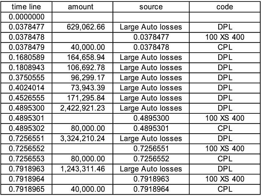
It can be seen that there are three more large losses, which respectively cede 80,000, 80,000, and 40,000. The last is less than 80,000 because the aggregate limit for the contract has been reached. Further losses would cede nothing.
It is also possible to step through a realization. On the sheet “Event History” click “Prepare.” This will go through the activated sheets and make sure they have all the needed ranges defined, as well as some other consistency checks. Click the “Initialize” button.[20] This will empty the timeline, and the cells labeled “next potential[21] event” will show what is waiting to happen. Going to the sheet which has the source “Large Auto Losses” on it (so far, there is only one random source, namely “simplest”) we can see the calculation that led up to the incurred value shown for the next potential event, starting with the gold cell with a random uniform value in it. Then back on “Event History” click “Step.” This will put the event on the timeline and bring up the next potential event. If the current event is large enough to exceed the $400,000 occurrence retention, then we will also see, as above, a “contract touched” event and a ceded loss (CPL) event. In order to see this, repeatedly click “Initialize” until the next potential event amount exceeds the retention, and then click “Step.” Going to the contract sheet “two year XS,” we can see all the calculations which created the ceded loss. As we repeatedly step and look at the contract sheet for each cession, we can see the annual totals being created. Again, for each event the complete calculation is available (until the next event is created).
Especially when stepping, it is convenient to change sheets by the “Go to generator” button. Clicking it will display an alphabetical dropdown list by either source name or sheet name. Highlighting a name and clicking “OK” will take you to that sheet. If you are on a sheet and its name is highlighted, clicking “OK” will take you back to the main sheet “Event History.” Other tips: if you get tired of stepping, you can click on “run to completion” to finish the realization; “toggle sources” will show additional information on the timeline.
It is also possible to show more detail on the timeline for more complex situations. In fact, anything of interest, including internal states of the generators, can be published on the timeline. Some situations require this information, as when a backup contract is used and needs to know when the backed-up contract has been exhausted or when a contract needs the policy limit of the loss.
On the “Reports” sheet to the left of “Event History,” we see the totals of various amounts of interest for this realization. The total DPL is $8,232,395.71; the total DPL discounted at 4% is $8,046,674.69. The discounting uses the actual times, of course. Figure 2 is an excerpt.
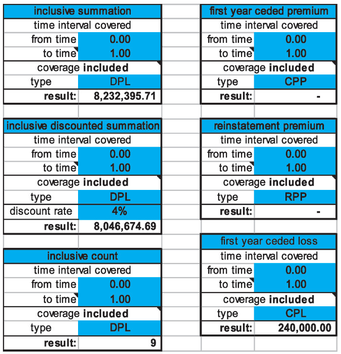
We can also see that we have no ceded premium, which means either that we got a very good deal from the reinsurer or that we probably need to extend the model.
In order to do a simulation, after having activated the appropriate sheets (and preferably done a few runs to make sure things are working correctly) we can select cells on the “Reports” sheet and then click on the “Simulate” button. This just repeats “Run” the desired number of times, and puts statistics and a cumulative distribution function on the sheet “Simulation Results,” which will be created if it is not present.
The sheet “simplest” has just the basic elements. The frequency is constant. The severity is ballasted Pareto (for the formula, see the sheet). The severity is conditional on the losses being between 50,000 and 10,000,000, since we are looking at just large losses. Various interesting measures about the severity are also on the sheet, including two moments and the cumulative probability distribution, both direct F(x) and inverse x(F). With x set to 400,000, the retention of the contract, we see that F(x) = 78.2% so that for any single Large Auto loss the probability of exceeding the retention and possibly generating a ceded loss is 21.8%.
This simplest form—a pure Poisson generator—is typically what is used when parameter uncertainty is ignored. There is no particular restriction to a Pareto severity; it was used here because it is both simple and typical for large losses.
Another point of note is on the contract sheet “two year XS” where we need some way of accumulating ceded losses to see the effect of the contract’s occurrence and annual limits. This is done by using VB code to write information from the current calculation into a cell for use by the next calculation of the spreadsheet. The reason it is done this way is to avoid a recursive formula which Excel could not handle. The area where it happens is labeled “changing state variables” because it contains variables relating to the state of the contract, which are necessary for the contract calculation and which are not fixed, unlike the limits and retentions.
To watch it work, click on the button “Initialize Recursion” to reset the accumulators to their initial values, in this case zero. Type 420,000 into the cell B8 labeled “current payment” and click on “Calculate.” This mimics the effect of an event with coverage being seen by the contract. It calculates everything to the left of the vertical double red lines. We will see the cell F22 labeled “current potential ceded” now contains 20,000. If the cell B11 labeled “occurrence time” contains a number between zero and one, then the cell I5 labeled “year 0 total—next” will also contain 20,000. The cell J5 labeled “year 0 total— current” contains zero. Now click on “Step Recursion” and see that “year 0 total—current” also contains 20,000. The sheet is now ready for the next calculation. Change the “current payment” to 430,000 and click on “Calculate” again. Then “current potential ceded” now contains 30,000 and “year 0 total—next” contains 50,000. If you click on “Step Recursion” again, then “year 0 total—current” also contains 50,000 and we are ready for the next event. The number of invocations tells how often the sheet has been calculated. This same procedure is followed on many sheets that need to retain information for subsequent use.
Note that this is a two-year contract. If we change the horizon on “Event History” to 2 and click “Run” we can see the results for both years.
5.2. Source interdependence and event codes
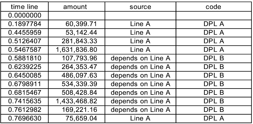
For a very simple example, click on “Activate Sheets” and select “Line A” and “Line B.” Line A is exactly the same as “simplest” except for the labels on the source name and on the output type. The output is “DPL A” which is just shorthand for direct paid loss from line A. The report summaries which are, as above, set to “included” will read any code that has “DPL” included in it as direct paid loss.
The line B source name is, unimaginatively, “depends on Line A.” Line B has again the same severity, but has a variable frequency depending on line A output. If the last line A loss is less than a threshold then the frequency is zero and there are no line B events; if it is greater than the threshold, then the frequency jumps to 30. With the threshold set to 1,000,000, by looking at the line A sheet where F(1, 000, 000) = 86.8% we may anticipate on average about one large event per run. Since the frequency of line A is 6, what we expect is an average of about 5 line B events for every large line A event.[22]
The user is encouraged to do a number of runs, and to play with the parameters to see how they influence the appearance of events on the timeline. One run generated this timeline shown in Figure 3.
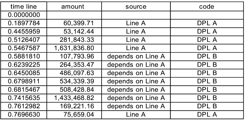
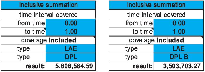
The reporting on DPL (and LAE, of which there is none) showed the sum of the amounts, and the report on DPL B gave just the line B amounts. In Figure 4 we can create reports on any event code.

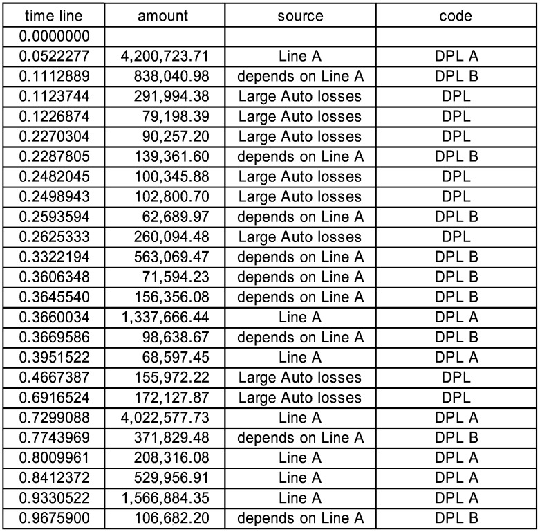
While there may not be an insurance situation with a dependency precisely like that of line B on line A, this simple example illustrates that if you can state the algorithm for the dependency in Excel you can simulate with it. The reader is encouraged to add Large Auto losses back in the mix,[23] and see that the auto losses and line A just act independently, whereas line B is always tied to line A output. The next timeline shows an example where some Large Auto losses occur in the middle of a set of line B losses because line A starts with a large loss and there is a long delay to a small loss in Figure 5.
5.3. Negative binomial, random payouts, and the schedule
This example, on the sheet “gamma mix,” has a negative binomial frequency. As usual, to see it run alone we must click “Activate” and select “gamma mix” while deselecting others. The negative binomial frequency is created by having an initial draw for the frequency from a gamma distribution. We specified the frequency parameters in terms of the mean frequency and the coefficient of variation of the mixing distribution and calculated the negative binomial moments, but we could as easily have done it the other way around. The severity is again Pareto.
Perhaps of more interest is the payout pattern. There is an initial payment, followed by a random number of randomly timed payments. To keep life a little simple, the amounts are all made the same. We could easily have made it even simpler by insisting that the payments only happen at fixed intervals after the claim occurrence, the way most simulations work now. The number of subsequent payments is Poisson[24] with mean 5.4, and the interval times between payments are exponential with mean 0.25. The source name is “Casualty 2” and the payment behavior is meant to have more of the randomness that might characterize a casualty line.
When the generator is invoked, the subsequent payments go to the schedule. We can see this by stepping through the realizations. On one particular timeline, after the first invocation the schedule shows in Figure 6.
After the next step, which is a new event before the next scheduled event, we see five new payments sorted into the schedule in Figure 7. The first part of the resulting timeline shown in Figure 8.
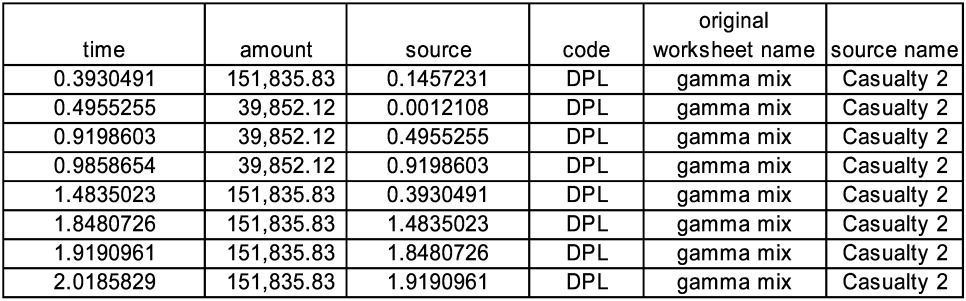

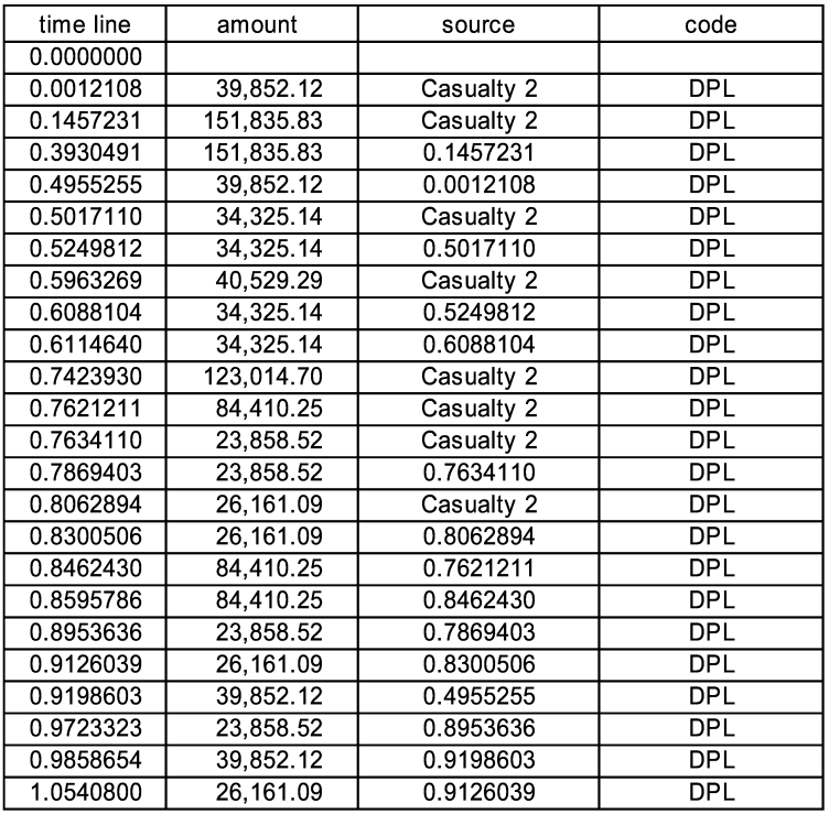
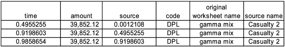
We can pick any one event, say the 23,858.52 loss at 0.9723323 and track back its sources through the preceding events at 0.8953636 and 0.7869403 to the original event of this cascade at 0.7634110. What you do not see at time 0.9723323 is that the last payment of this series is actually at 3.0050366. In the spreadsheet if we click “Toggle Sources” we see the column labeled “original source event.” There is a filter set up on this column, and we can filter on the original source event and see the whole cascade in Figure 9.

As alluded to above, the intent of the “source” column is to provide an audit trail whose metaphor is that of picking up one bead on a string and being able to follow the string back to the original source. Every event either connects to a prior event labeled by its time, or is an original event from a random or scheduled source.
5.4. Exposure and scheduled events
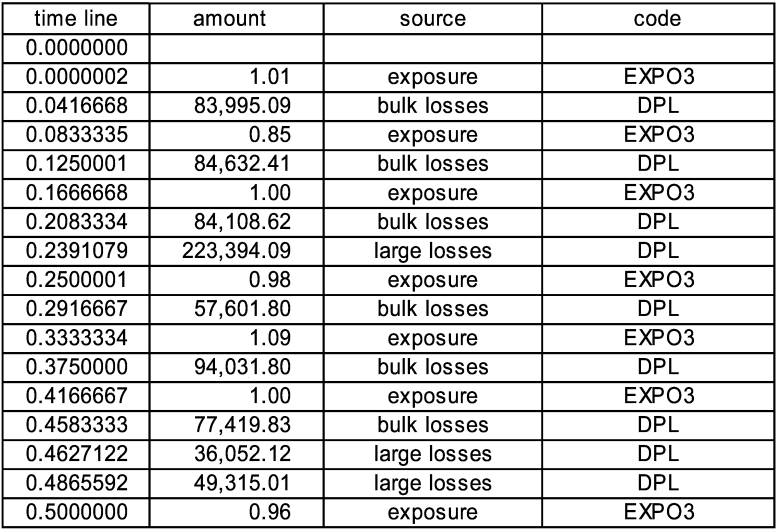
The sheet “exposure” has an exposure which is stochastic about a time-dependent mean value. The sheet “exposure-driven freq” has a loss frequency which is proportional to the exposure. The sheet “monthly aggregates” uses the same exposure as a factor on its mean severity. The latter two sheets use the function GetMostRecentValue(code, default value), which is available to any worksheet, for looking at the timeline. This function is also used in the example of Section 5.2 and many other sheets. The intent here is to provide a simple example for an exposure-driven model of both large losses and bulk aggregation of small losses. The large losses are modeled as having an immediate payment resulting from a Beta distribution applied to the total and a second payment of the remainder at a random time later. Currently the mean of the Beta is 60% and the mean time to the second payment is 1.2 years, but of course these can be changed to anything desired.
One timeline begins as in Figure 10. Since the amount column is formatted for dollars and cents, we see the exposure index rounded to two figures although its complete value is used in calculation. The schedule plays a slightly different role here, because while the times for the bulk losses are known at the beginning, the amounts are To Be Determined (TBD). If we click “Initialize” and then look at the schedule we will see in Figure 11.

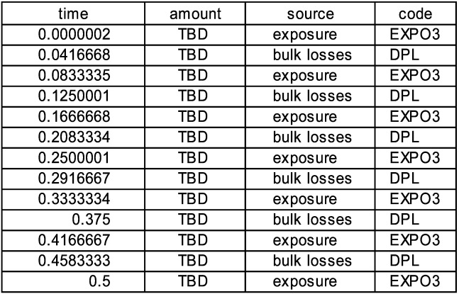
During subsequent steps, at the appropriate time, the source is called to do a calculation and create the current amount. For the exposure the source can simply create the amount, but for the bulk losses the source must look back in history to see the current exposure value. A similar look back is done when the frequency for the large losses is polled in order to find the next event.
5.5. Loss generation with full uncertainty
The sheet “full uncertainty” is a loss generator with a basic form that is negative binomial with a Pareto severity. However, it has various forms of parameter uncertainty represented as well. The initial calculation draws from a parameter distribution specified by the uncertainties of the negative binomial and Pareto distributions, which come from a curve-fitting routine. The calculation then adds a projection uncertainty to account for uncertainties in the on-leveling, missing data, environmental changes, etc. The latter is mostly subjective and dependent on the individual company and line of business. This draw from parameter distributions is, as discussed before, either a reflection of our ignorance or a reflection of the complexity of the world, depending how we think of it. In any case, what is essential is that the draw be done only at the beginning of each realization, and not every time the frequency or severity distribution is used. The parameters remain the same throughout the realization, and only change for the next realization.
It is worth noting how the initial choice of parameters is done. This whole calculation is to the right of the double red lines. If we click the button “Initial Calculation” we can see the various random choices being made and the resulting frequency and severity parameters. This feature is also present in the previously used sheet “gamma mix” and many others. There is a range “calc initially” (which can be seen by using the “Edit-Go To” command on the Excel menu) that is calculated by the VB code initially or by clicking the button “Initial Calculation.”
This sheet also generates a random number of payments, each some random fraction of the current outstanding value, at random times. In the end, any one timeline is still a set of dollar loss amounts at different times, so it does not look very different from what we have seen. However, being able to model the uncertainties explicitly will give fairly different results from using just the simple form at the modal values, especially in the tail.
This sheet also publishes additional detail, namely the current outstanding value for each loss at each payment time. This is needed for some contracts, such as the European index clause.
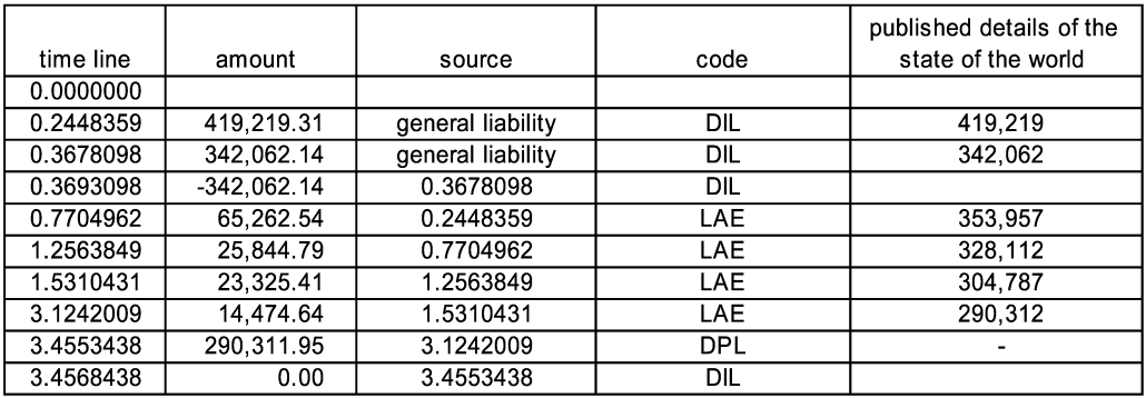
5.6. A general liability model
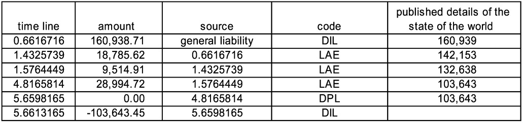
Well, sort of. The sheet “General Liability” is similar to the above in the uncertainties and is meant to be a suggestion toward a model of loss and legal fees by paying legal fees and then either winning or losing in court. There is an initial direct incurred loss (DIL), and then typically a stream of relatively small loss adjustment expense payments (LAE) followed by a large direct paid loss (DPL) with no change in the incurred value. Sometimes there are no payments, and there is a takedown of the incurred. There are a variable number of payments (the mean number increases with the claim size) at random times with a mean delay between them of 0.5, and the legal payment totals are about 30% of the original incurred. The larger claims, having more payments on average, will tend to take longer to settle since the mean delay time is fixed. At the end, there is a “good lawyer” parameter. If the final outstanding is less than this parameter, the (high) legal fees are presumed successful and the final payment is zero, with a takedown in the incurred occurring one half day after the final payment.
Figure 12 shows a sample timeline showing a typical claim and a close without payment claim. The published details are the current outstanding value for the combined loss and LAE claim.
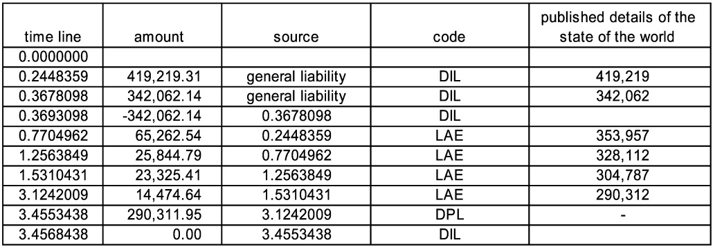
Figure 13 shows a claim where the good lawyer prevailed. This is a timeline filtered on the original event.
5.7. Loss generation from policy limits
The sheet “Property w Policy Limit” contains a policy limit profile. It generates a loss amount using a beta distribution with a large standard deviation times a factor greater than one, and limiting the result to one, and multiplying by a randomly chosen policy limit. This results in the classic shape of a property curve with many small losses and an uptick at very large losses. In a separate simulation, the mean and standard deviation of the policy limits, the percentage of policy limit, and the loss amounts are generated to confirm the desired behavior.
When the loss generation is based on estimated exposure rather than on a specific policy limit, the percentage drawn should not be capped at one, so that losses beyond the estimated exposure are allowed. The same could also be said for losses beyond policy limit, depending on the situation.
5.8. Multiple part contract
The example is a surplus share corridor, which could actually have been done on a single sheet but is done this way to show again how generators can communicate via events on the timeline. The three sheets which must be activated (in addition to “Property w Policy Limit,” which is the source of loss to which they apply) are “Surplus Share Corridor.A,” “Surplus Share Corridor.B,” and “Surplus Share Corridor.” Parts A and B are standard surplus share contracts which also have aggregate limits, and the corridor itself is the sum of the two. The aggregate coverages are 5M excess 5M on part A, and 5M excess 15M on part B, leaving open the corridor 5M excess 10M for the cedant. Both Part A and Part B are nine line coverages with a 1M retained line. This means that on a 1M policy, they cede nothing, on a 2M policy they cede 50%, on a 5M policy they cede 80%, on a 10M policy they cede 90%, etc.
There are several interesting features. First, the surplus share contracts need to know the policy limit in order to calculate the cession percentage. To do this, the Property source publishes the policy limit as an interesting loss detail. Then parts A and B look at the loss and the policy limit, and produce LOSS.A and LOSS.B. The corridor itself picks these up as well as the policy limit and creates a ceded loss.
One timeline, shown in Figure 14, where the large losses used up all aggregate limits, first in part A and then in part B.
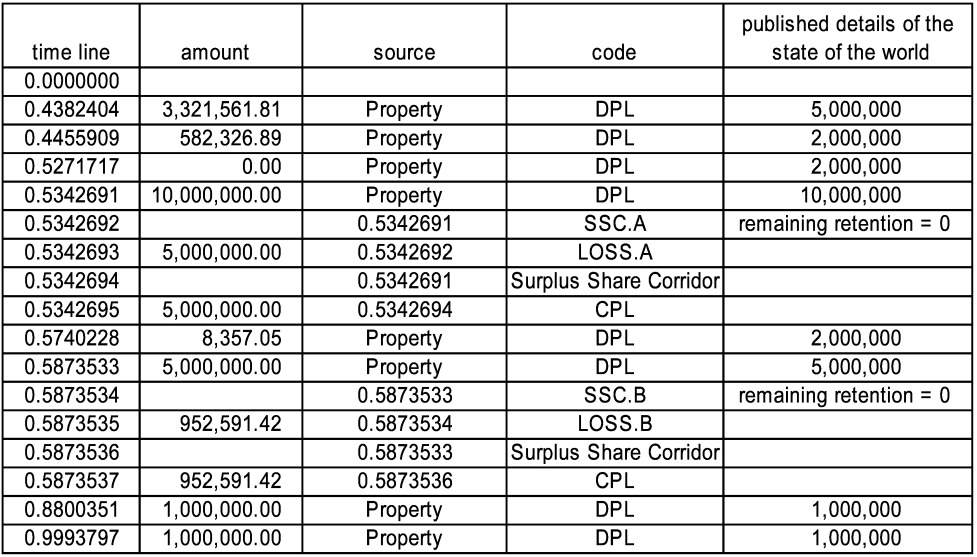
Note that each loss also carries with it the corresponding policy limit, which the surplus share contracts need to do their calculation. They access it using the function OriginalLossDetail.
5.9. Stochastic premiums
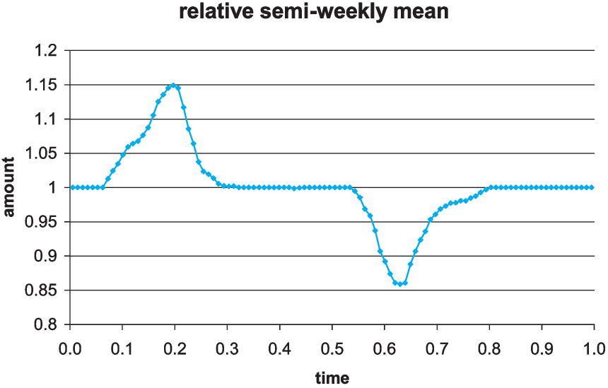
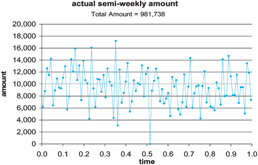
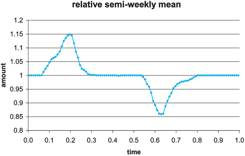
In this example we know the relative planned amounts on a semiweekly basis and want to generate random premium or other entries. Basically, this is meant to show how to use the schedule to include quite complicated random inputs in the simulation. Here we want random entries whose sum has a given mean and coefficient of variation. The sheet “direct premiums” has 104 random entries with specified relative means, and generates them as deviates from a normal distribution whose parameters are chosen to give the desired overall results on average. Although these are stated as premiums, these events could be time-signals or exposure measures to modify frequencies, for example. If we think of this as written premium, we can earn it out over time. Here, the specified mean is 1,000,000 and its coefficient of variation is 3%. The following is the underlying variation of the mean values, with a peak in the spring and a dip in the fall in Figure 15. Figure 16 shows one realization produced. It would be hard, looking at this as data, to infer the actual underlying 15% rise in spring and 15% drop in late summer of the relative means.

5.10. Cats, copula, cat cover, and inurance
The sheet “hurricane” is a catastrophe modeled as three Pareto severities connected by a copula. This sheet will give separate events for Florida, Georgia, and South Carolina. It also puts out events for the start and end of each cat. The hurricane season is modeled as having uniform frequency from August through October, but clearly we can do better than that and put in more accurate seasonality. On the timeline, there are events to start and end the season.
The sheet “cat cover” is a contract for 50,000,000 excess of 50,000,000 with one free reinstatement and 95% participation on the total loss from each cat. There is a Florida-only contract and the sheet “FL excess” inuring to it which has one reinstatement at 100%. This contract has ceded paid premium (CPP) and reinsurance paid premium (RPP), the latter being the premium paid for reinstatement.
It should be noted that contracts are evaluated in workbook order, and a contract which inures to another must be evaluated first. Hence “FL excess” must precede “cat cover.” Figure 17 is one timeline.
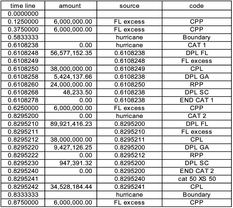
The ceded paid premiums occur at the middle of each quarter. It might be mentioned that the cat cover itself is apparently free, since there is no ceded premium for it. The events at .583 and .833 are meant to express the boundaries of the hurricane season and change the frequency on the loss generator. The events noting the end of each cat are used in the cat contract to aggregate the losses less the inuring loss on the Florida portion and pay (or not) on the total.
5.11. Other examples
The European index clause in some of its incarnations is sheet “Euro indexed XS.” This clause requires more timeline look-ups than any other so far, since it needs to know external indices and times of various events in order to do its calculation. The source to which it refers, “uniform mix,” is where the frequencies are randomly chosen from a uniform distribution on a specified range. There is a random number of payments for each loss, at random times. The excess contract uses the times and the current outstanding values, as well as the current index value. The index is on the sheet “index” and is lognormal. It must create values at least as far out on the timeline as the last payment, and so the checkbox “Initial Schedule past Horizon” on the sheet “Event History” needs to be checked.
The sheet “freq pdf” allows an arbitrary density function for the frequency, assigning random times during the years to randomly drawn numbers of annual events. It also allows for a Horizon which is not an integer. At the moment it does at most three years.
The sheets “XOL w Backup” and “Backup on XOL” are, respectively, an excess of loss contract which has a backup, and the backup contract. The former puts out an event with code CBL, for ceded backup loss. Again, there is no restriction on what may be a valid code, and the user is invited to create any codes which may be helpful in her particular problem. The applicable loss is “Property” and the sheet generating it is “Property w Policy Limit.” Because the backup contract may be dealing with only a partial payment from the contract it backs up, it needs the function “AmountFromContractOnCurrentEvent.”
The sheets “Time by loss” and “Loss by time” are two slightly different ways of implementing the presumption that large losses close later than small losses on average. In both sheets, there is a single payment at some random time after the incurred loss. In the former, the mean of the (exponential) time distribution is proportional to a power of the ratio of the random loss to its mean. In the latter, the severity mean is a power of the random time to pay to its mean. These correspond to the intuitions that (1) if a claim is large, then it will usually close later (perhaps because we will fight it in court); or (2) if a claim takes a long time to pay, it is probably large (perhaps because the court case is complex). The point here is that you can model either way quite easily with only a few parameters, rather than with many. The author would love to see someone with data actually parameterize and validate or invalidate these models, and then build something that can be used.
There is a contagion example on the “contagion” sheet, where the presence of a claim increases the probability of more claims. Here the frequency is linear in the counts, and results in a negative binomial at any point in time, the mean of which exponentially increases with time. For a mass tort situation, it might make more sense to have a very low frequency which increases nonlinearly in the number of claims to a maximum. Perhaps it even decreases again later.
There are a few more sheets illustrating miscellaneous things: how to put in historical (or any fixed) losses, how to have an exact number of losses, a simple version of stochastic reserves, a quota share contract with insurances, a contract on just the largest three claims, and finally a contract which is only active on September 11 of any year.
6. Epilogue
The suggested conclusion is “try it, you’ll like it.” There is much more control over interacting events in a timeline formulation, and it is easier to express intuitions.
However, there are very few actuarial models which work on this level. The big challenge is to create and then parameterize such models, starting with doing maximum likelihood on actual time delays.
A case in point is accident year data. One useful model is that an accident occurs at a random time during a year, and then there is a single payment whose time delay from occurrence also has a random distribution. The accident year data is the time from zero to payment, which is the sum of the time to occurrence plus the payment delay, and thus the convolution of two random variables. Since our data comes in this form, we need to be able to produce a payment time delay distribution by fitting to it.
Clearly, one solution (which corresponds to the collective risk model) is to say that for accident year data, payments either happen when the accident occurs, exactly one year afterward, exactly two years after, and so on with no payments at other intermediate times. However, it is hard to believe that this is how a claims department actually works. Another solution has been found, using a piecewise linear continuous payment distribution. It is usually possible to fit a payment pattern exactly, but that can result in an unreal density, especially for payments on high excess contracts. Compromising between the quality of the fit and a smoother payment density results in graduated payout patterns. An additional virtue of this procedure is that the calculations can be done exactly for the case where, say, the first accident year is only seven months of data. Ordinarily we would multiply by 12/7 or use some interpolation procedure as a guess, but we can actually evaluate the payout probabilities over any time interval, rather than just whole years or quarters. If we had not been thinking in terms of timelines, this whole graduation approach—which can be used in non-timeline problems—would not have occurred to us.