Interval Estimation of the Credibility Factor

undefined

1. Introduction

Credibility modeling is a ratemaking process which allows actuaries to adjust future premiums according to past experience of a risk or group of risks. For instance, Herzog (1994) considered two sets of data. The first is the collection of current observations from the most recent period. The second is the collection of observations from one or more prior periods. Under some credibility approaches, the new rate, C (for claim frequency, claim size, aggregate claim amount, etc.), is calculated by:

\[ C=Z \times R+(1-Z) \times H, \tag{1} \]

where R is the mean of the current observations, H is the mean of the prior observations, and Z is the credibility factor, ranging from 0 to 1. The credibility factor Z denotes the weight assigned to the current data and (1 − Z) is the weight assigned to the prior data. Zero credibility (Z = 0) will be assigned to data too small to be used for ratemaking, while full credibility (Z = 1) is assigned to fully credible data.

Bailey (1950) showed that the formula ZR + (1 − Z)H can be derived from Bayes’ theorem, either by using a Bernoulli-Beta model on the unknown parameter p, or by using a Poisson-Gamma model on the unknown parameter λ. Bailey’s work led to the application of Bayesian methodology to credibility theory. Bayesian statistical analysis for a selected model begins by first quantifying the existing state of knowledge and assumptions. These prior inputs are then combined with information from observed data quantified probabilistically through the likelihood function. The mechanism of prior and likelihood combination is Bayes’ theorem. In technical terms, the posterior is proportional to the prior and the likelihood, i.e.,

\[ \text { posterior } \propto \text { prior } \times \text { likelihood. } \]

However, the prior distributional assumptions in Bailey’s models were severely limited. Bühlmann (1967) overcame these limitations and proved that Equation (1) is also a distribution-free credibility formula. The best linear approximation of this formula is found by minimizing
\(E\left\{E\left[\mu(\theta) \mid x_1, \ldots, x_n\right]-(a+b \bar{X})\right\}^2\), where \(\mu(\theta)\) is the mean of an individual risk (or the hypothetical mean \(E\left(X_i \mid \theta\right)\) ), characterized by a risk parameter \(\theta\), and \(\bar{X}=\left(x_1+x_2+\cdots+x_n\right) / n\). Additionally, the process variance, \(v(\theta)\), is defined as \(\operatorname{Var}\left(X_i \mid \theta\right)\). Bühlmann and Straub (1970) then formalized the least squares derivation of

\[ Z=n /(n+k), \tag{2} \]

where n is the number of trials or exposure units and

\[ k=\frac{v}{a}, \tag{3} \]

in which \(v=E[v(\theta)]\) and \(a=\operatorname{Var}[\mu(\theta)]\). Here, \(v\) and \(a\) are also known as the expected value of the process variance and the variance of hypothetical mean, respectively. This methodology is called empirical Bayes credibility, although the Bayesian content of this approach has been greatly minimized.

In practice, we have to estimate \(v\) and \(a\) to determine the credibility factor \(Z\). Naturally, actuaries use unbiased estimators of \(v\) and \(a\), denoted as \(\hat{v}\) and \(\hat{a}\) respectively. When a sample of claims is available, \(\hat{v}\) and \(\hat{a}\) are then realized. However, actuaries traditionally stop at a point estimate without considering possible variation caused by a random sample. Therefore, we take a Bayesian approach and treat the unknown quantities \(v\) and \(a\) as random variables. This allows us to estimate \(v, a\), and \(Z\) simultaneously and allows the assessment of the credibility factor in terms not only of point estimators, but also of certain characteristics of probability distributions.

To date, Bayesian methodology has been used in various areas within actuarial science. Klugman (1992) provided a Bayesian analysis to credibility theory by carefully choosing a parametric conditional loss distribution for each risk and a parametric prior. To be useful in public discussion, such a prior must be evidence-based in some sense, e.g., be a summary of an expert’s opinion on the topic. Bayesian methods provide a natural way to incorporate this prior information, whether statistical or not, in the form of tables or as expert judgement, through the prior distribution of the parameters.

In many cases, Bayesian methods can provide analytic closed-formed solutions for the posterior distribution and the predictive distribution of the variables involved. Then, the inference is carried out directly from these distributions and any of their characteristics and properties. However, if the distribution is not a known type, or if it does not have a closed form, then it is possible to derive approximations by means of Markov chain Monte Carlo (MCMC) simulation methods.

In summary, MCMC algorithms construct the desired posterior distributions of the parameters. Thus, when convergence is reached, it provides a sample of the posterior distribution that can be used for any posterior summary statistics of interest. Details of the technicalities involved in MCMC can be found in Smith and Roberts (1993) or in Gilks, Richardson, and Spiegelhalter (1998). MCMC algorithms have appeared in actuarial literature by de Alba (2002), Carlin (1992), Frees (2003), Gangopadhyay and Gau (2003), Ntzoufras and Dellaportas (2002), Rosenberg and Young (1999), and Scollnik (2001). The advantage of using this procedure is that actuaries can obtain point estimates as well as probability intervals and other summary measures, such as means, variances, and quantiles.

In this article, we provide an alternative method for calculating the credibility factor, particularly the interval estimation of the credibility factor. There is a range of concerns that arise in credibility modeling. We present an effective method to deal with these concerns. Section 2 introduces the credibility problem. Section 3 uses a simulated example to illustrate the basic idea of the Bayesian credibility factor. Section 4 discusses the advantages and disadvantages of the Bayesian credibility factor. Remarks are made in Section 5.

2. Credibility problem

The classical data type in this area involves realizations from the past and present experience of individual policyholders. Suppose there are \(r\) different policyholders. We have a claims record in year \(j, j=1, \ldots, n_i\), for policyholder \(i, i=1, \ldots, r\). Therefore, the data can be summarized in the following form,

\[ \begin{array}{l} X_{11}, X_{12}, \ldots, X_{1, n_{1}} \\ X_{21}, X_{22}, \ldots, X_{2, n_{2}} \\ \ldots \ldots \ldots \ldots \ldots \\ X_{r 1}, X_{n 2}, \ldots, X_{r, n_{r}}, \end{array} \tag{4} \]

where \(X_{i j}\) can be the losses per exposure unit, the number of claims, or the loss ratio from insurance portfolios. The goal is to estimate the amount or number of claims to be paid on a particular insurance policy in a future coverage period.

2.1. Variance component models

Dannenburg, Kaas, and Goovaerts (1996) introduced the use of variance component models to the credibility problem. In a variance component model, each cell (policyholder \(i\) in year \(j\) ) consists of a number of contracts \(m_{i j}\), which has been observed over a number of observation periods \(n_i\) for contract \(i\). Then, for the \(i\) th contract in the portfolio, \(i=1, \ldots, r\), in year \(j=1, \ldots, n_i\), the claim experience is represented by the model

\[ \begin{aligned} X_{i j} & =\mu+\alpha_{i}+\varepsilon_{i j}, \\ i & =1, \ldots, r \quad \text { and } \quad j=1, \ldots, n_{i} \end{aligned} \tag{5} \]

where \(\alpha_i\) and \(\varepsilon_{i j}\) are independent with \(E\left[\alpha_i\right]=0\), \(\operatorname{Var}\left[\alpha_i\right]=a\) and \(E\left[\varepsilon_{i j}\right]=0, \operatorname{Var}\left[\varepsilon_{i j}\right]=v / m_{i j}\) for all \(i\) and \(j\).

In order to determine the credibility factor and the credibility premium, we need to estimate parameters \(\mu, v\), and \(a\). In general, the unknown parameters \(\mu, v\), and \(a\) are associated with the structural density, say \(\pi(\theta)\), and hence we refer to these as structural parameters. For the Bühlmann and Straub (1970) formulation, the hypothetical mean is defined as \(E\left(X_{i j} \mid \Theta_i=\theta_i\right) \equiv \mu\left(\theta_i\right)\) and the process variance is defined as \(\operatorname{Var}\left(X_{i j} \mid \Theta_i\right.\) \(\left.=\theta_i\right) \equiv v\left(\theta_i\right) / m_{i j}\). Thus, the structural parameters are given by

\[ \mu=E\left[\mu\left(\Theta_{i}\right)\right], \quad v=E\left[v\left(\Theta_{i}\right)\right], \tag{6} \]

and

\[ a=\operatorname{Var}\left[\mu\left(\Theta_{i}\right)\right] . \tag{7} \]

Consequently, the credibility factor \(Z_i\) for each risk is given by

\[ Z_{i}=\frac{m_{i}}{m_{i}+k}, \tag{8} \]

where

\[ k=\frac{v}{a} \tag{9} \]

and

\[ m_{i}=\sum_{j=1}^{n_{i}} m_{i j}, \quad i=1, \ldots, r. \tag{10} \]

2.2. Traditional credibility modeling

If estimators of \(\mu, v\), and \(a\) are denoted by \(\hat{\mu}, \hat{v}\), and \(\hat{a}\), respectively, then the resulting credibility premium is given by

\[ \hat{P}_{i}=\hat{Z}_{i} \bar{X}_{i}+\left(1-\hat{Z}_{i}\right) \hat{\mu}, \quad i=1, \ldots, r, \tag{11} \]

where

\[ \hat{Z}_{i}=\frac{m_{i}}{m_{i}+\hat{k}}, \tag{12} \]

\[ \hat{k}=\frac{\hat{v}}{\hat{a}}, \tag{13} \]

and

\[ \bar{X}_{i}=\frac{\sum_{j=1}^{n_{i}} m_{i j} X_{i j}}{m_{i}}, \quad i=1, \ldots, r . \tag{14} \]

Today, one of the most widely used methodologies for the choice of \(\hat{\mu}, \hat{v}\), and \(\hat{a}\) is empirical Bayes parameter estimation. It allows us to use the data at hand to estimate the structural parameters. The resulting estimators are

\[ \hat{\mu}=\bar{X}=\frac{\sum_{i=1}^{r} m_{i} \bar{X}_{i}}{m}, \tag{15} \]

\[ \hat{v}=\frac{\sum_{i=1}^{r} \sum_{j=1}^{n_{i}} m_{i j}\left(X_{i j}-\bar{X}_{i}\right)^{2}}{\sum_{i=1}^{r}\left(n_{i}-1\right)}, \tag{16} \]

and

\[ \hat{a}=\frac{\sum_{i=1}^{r} m_{i}\left(\bar{X}_{i}-\bar{X}\right)^{2}-(r-1) \hat{v}}{m-\frac{\sum_{i=1}^{r} m_{i}^{2}}{m}}, \tag{17} \]

where \(m=\sum_{i=1}^r m_i\). Note that Equations (15), (16), and (17) are unbiased estimators of \(\mu, v\), and \(a\), respectively.

However, there are some issues raised from traditional credibility modeling. First, the estimate of \(a\) can be negative, a clearly unacceptable value. The second issue is the need for obtaining a measure of the quality of the credibility estimate. The measure of error for Equation (11) depends on \(a, v\), and the credibility factor \(Z\). None of the standard approaches to credibility analysis provides a method of accounting for this extra variability.

3. A simulated example

In this section, we consider an example based on data simulated from a normal distribution. It is always a concern with this assumption in credibility modeling due to the likelihood of a heavy tail in loss distributions. However, the normal model is still a very useful approach in many problems. For non-normal data, we will recommend a data transformation before using a more sophisticated model. Variable transformations serve a variety of purposes in data analysis and are used in particular to make distributions more symmetric (or normal), to stabilize variation, and to render relationships between variables more nearly linear. These techniques can be found in Box and Tidwell (1962), Box and Cox (1964), and Klugman (1992).

Based on Equation (5), it is assumed that

1. \(\mu=200\).
2. \(\alpha_i\) has a normal distribution with mean 0 and variance 400 (i.e., \(a=400\) ).
3. \(\varepsilon_{i j}\) has a normal distribution with mean 0 and variance 2500 (i.e., \(v=2500\) ).

Specifically, the data is generated using the following mechanism:

1. \(\theta_i \stackrel{\text { i.i.d. }}{\sim} N(200,400)\).
2. \(X_{i j} \mid \theta_i \stackrel{\text { i.i.d. }}{\sim} N\left(\theta_i, 2500\right)\).

We consider a portfolio of five policyholders with five years of experience. There is only one claim every year for each policyholder. That is \(r=5, n_i=5\), and \(m_{i j}=1\) in Equation (5). Using Equations (8), (9), and (10), we have the true credibility factor

\[ Z=\frac{5}{5+\frac{2,500}{400}}=0.4444 . \tag{18} \]

Table 1 shows simulated data from the above settings, in which \(\theta_i=\mu+\alpha_i\). Using Equations (15) to (17), we have \(\hat{\mu}=200, \hat{v}=2684\), and \(\hat{a}=\) - 201. Traditionally, actuaries will set \(\hat{a}\) to be zero when \(\hat{a}\) is negative. Thus, the credibility factor is calculated as

\[ \hat{Z}=\frac{5}{5+\frac{2684}{0}}=0 . \tag{19} \]

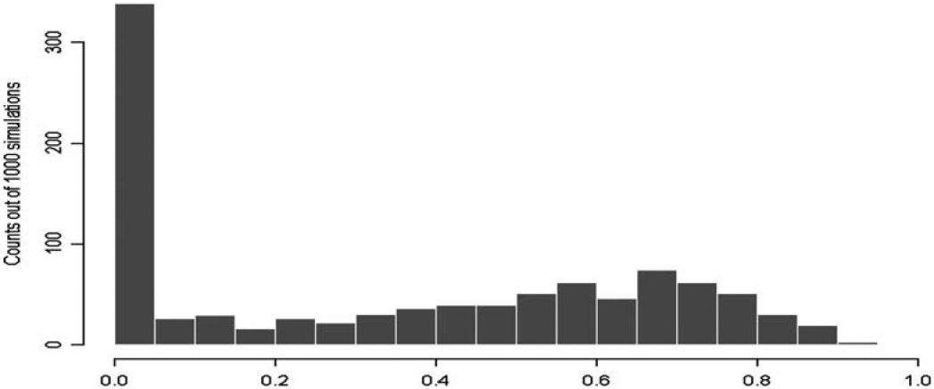
Clearly, this is a situation in which traditional credibility factor analysis does not perform well. Figure 1 shows the histogram of credibility factors based on 1000 simulated portfolios. There are a large number of simulated portfolios (about 300 out of 1000), resulting in a zero credibility factor due to a negative value of â.

3.1. Bayesian credibility factor

As seen previously, a negative value of â is a major drawback of this unbiased estimator. Therefore, we seek other alternatives to estimate the credibility factor Z. The Bayesian method and the MCMC technique can be applied with objective selection of a model structure and prior distributions based on actuarial judgment.

In this section, we will focus on the variance components model introduced in Equation (5). A general introduction to Bayesian inference on variance components can be found in Searle, Casella, and McCulloch (1992). Bayesian credibility factors in actuarial applications are introduced in Appendix A. The benefit of a Bayesian approach is that it provides the decision maker with a posterior distribution of the credibility factor as well as a posterior distribution of the premium.

In actuarial science, both outcomes and predictors are often gathered in a nested or hierarchical fashion (for example, fires within counties within states, employees within companies within industries, and patients within hospitals). Thus, as observed by various researchers in actuarial science, hierarchical models are ideally suited to the insurance business in which single- or multi-stage samples are routinely drawn. A number of examples can be found in Klugman (1992) and Scollnik (2001).

For the simulated example, we use the following hierarchical setting.

1. \(X_{i j} \mid \theta_i, v \sim N\left(\theta_i, v\right)\).
2. \(\theta_i=\mu+\alpha_i\).
3. \(\theta_i \mid \mu, a \sim N(\mu, a)\).
4. \(\mu\) is an unknown constant, estimated by \(\hat{\mu}\) in Equation (15).
5. \(a \sim \operatorname{Gamma}\left(\alpha_a, \beta_a\right)\).
6. \(v \sim \operatorname{Gamma}\left(\alpha_v, \beta_v\right)\).
7. The Bayesian credibility factor is given by Equation (25) in Appendix A.

The Bayesian approach is a powerful formal alternative to deterministic and classical statistical methods when prior information is available. The choice of prior is often presented as an aspect of personal belief. In Appendix B, we present an empirical Bayesian approach for priors of \(v\) and \(a\).

Based on Equations (37) and (38) in Appendix B , we have \(\alpha_v=\sum_{i=1}^r\left(n_i-1\right) / 2=10\) and \(\beta_v=\) \(\alpha_v / \hat{v}_{\text {init }}=10 / \hat{v}_{\text {init }}\). The parameters for the prior distribution of \(a\) are given by \(\alpha_a=(r-1) / 2=2\) and \(\beta_a=\alpha_a / \hat{a^{\prime}}_{\text {init }}=2 / \hat{a}^{\prime}_{\text {init }}\) as shown by Equations (39) and (40) in Appendix B.

Using the simulated data in Table 1, we have \(\hat{v}_{\text {init }}=2684\) and \(\hat{a}_{\text {init }}^{\prime}=336\). Therefore, \(\beta_v=10 / 2684=0.0037\) and \(\beta_a=2 / 336=0.0059\). The estimation of the credibility factor Z, implemented with WinBUGS (Spiegelhalter et al. 1996), is summarized in Table 2.

The Bayesian approach suggests that the Bayesian credibility factor, \(\hat{Z}_B\), is the mean of the posterior distribution as indicated in Equation (25). Thus, we have \(\hat{Z}_B=0.2985\). Nevertheless, actuaries must recognize a possible variation inherent in the estimation of the credibility factor as shown in Table 2. Clearly, Table 2 gives us a more desirable result compared with the result from Equation (19).

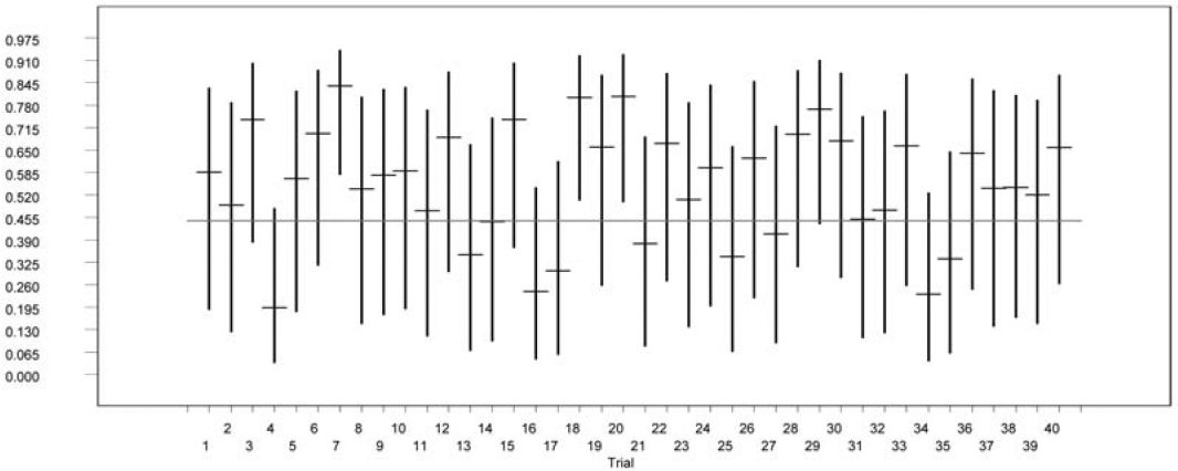
To assess the accuracy of the Bayesian credibility interval estimator, we simulate 40 portfolios from the normal-normal model with υ = 50² and a = 20²; and we construct a 95% credible interval for each portfolio based on the posterior distribution of the Bayesian credibility factor. These credible intervals are shown in Figure 2, where the horizontal line is the true credibility factor Z = 0.4444 and the dash line is the median of the posterior distribution of the Bayesian credibility factor. The true credibility factor falls in the credible interval 37 times out of 40 trials. For a detailed introduction to using WinBUGS in actuarial applications, the reader is referred to Scollnik (2001).

4. Further analysis

In this section, we extend our analysis to the advantages and disadvantages of the Bayesian credibility factor proposed in this article. What makes credibility theory work is that it results in a significant improvement in mean-squared error, even though the resulting credibility premium given by Equation (11) is a biased estimator. We expect that the biases will cancel out over the entire estimation process.

4.1. Sampling distribution

One advantage of the Bayesian credibility factor approach is its ability to describe the variation inherent in the process of estimating the credibility factor. Traditionally, actuaries use Equation (12) to determine the credibility factor for each policyholder and speak in absolute rather than probabilistic terms. After the credibility factor has been determined, actuaries usually treat it as a known constant.

However, the credibility factor estimator itself has a sampling distribution associated with it. That is, a realization of the credibility factor estimator in Equation (12) depends on the sample (or portfolio) drawn from the underlying population. This concept can be seen from Figure 1 and is summarized in Table 3.

Obviously, different simulated portfolios result in different values of the credibility factor. It is known that the impact of variation in the credibility factor estimator diminishes as the amount of experience grows (see Mahler and Dean, Graph 8.6 on page 597, 2001). However, we apply the credibility theory mostly because the data at hand is sparse, and we combine the limited data with other information. This is the concept embedded in Equation (1).

On the other hand, the Bayesian approach allows us to describe the phenomenon seen in Table 3. From Section 3.1, the Bayesian credibility factor approach suggests the mean of the posterior distribution as the best estimate of the credibility factor, i.e., \(\hat{Z}_B=0.2985\). At the same time, it also suggests that there is possible variation in the estimation process.

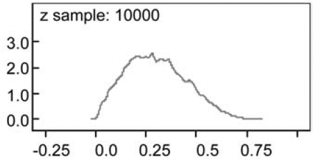
For the simulated example in Table 1, the Bayesian credibility factor approach is able to suggest that we are 95% sure that the true credibility factor will fall into the interval from 0.0511 to 0.6026. Additionally, the posterior distribution of \(\hat{Z}_B\) for the simulated data in Table 1 can be visualized in Figure 3.

4.2. Traditional credibility factor versus Bayesian credibility factor

Now, we want to demonstrate that the Bayesian credibility process can further improve the mean-squared errors in determining the credibility factor and the credibility premium. To see how this improvement comes about, we use the normal-normal model in Section 3 to simulate 50 trials (or portfolios). For each trial, simulated data is generated the same way as data in Table 1.

We first compare the traditional credibility factor \(\hat{Z}\) given by Equation (12) to the Bayesian credibility factor \(\hat{Z}_B\) suggested by Equation (25) in Appendix A. We use squared error as our criterion. The results are shown in Table 4, in which, \(\mathrm{SE}_{\hat{Z}}\) is calculated as \((\hat{Z}-0.4444)^2\) and \(\mathrm{SE}_{\hat{Z}_B}\) is equal to \(\left(\hat{Z}_B-0.4444\right)^2\). Note that the normalnormal simulation in Section 3 has a true credibility factor of 0.4444 . For data in Table 1, we have \(\mathrm{SE}_{\hat{Z}}=(0-0.4444)^2=0.1975\) and \(\mathrm{SE}_{\hat{Z}_B} =(0.2985-0.4444)^2=0.0213\). This is shown in trial 49 of Table 4. The interesting part is the significant improvement to mean-squared errors that result from the Bayesian credibility factor.

Our next task is to compare the traditional credibility premium \(\hat{P}_i\) provided by Equation (11) to the Bayesian credibility premium \(\hat{P}_i^B\), where

\[ \hat{P}_{i}^{B}=\hat{Z}_{i}^{B} \bar{X}_{i}+\left(1-\hat{Z}_{i}^{B}\right) \hat{\mu}, \quad i=1, \ldots, r . \tag{20} \]

For each simulated trial, we have \(\Theta=\left(\theta_1, \theta_2, \theta_3\right.\), \(\theta_4, \theta_5\)), which represents the true underlying individual premiums. For example, \(\Theta\) is given by (197, 201, 202, 208, 207) for the simulated data in Table 1. The sum of squared errors for the traditional credibility premium \(\hat{P}_i\) is defined as

\[ \sum_{i=1}^{5}\left(\hat{P}_{i}-\theta_{i}\right)^{2} . \tag{21} \]

The sum of squared errors for the Bayesian credibility premium \(\hat{P}_i^B\) is defined as

\[ \sum_{i=1}^{5}\left(\hat{P}_{i}^{B}-\theta_{i}\right)^{2} . \tag{22} \]

For the simulated data in Table 1, we have \(\hat{P}_1=\) \(\hat{P}_2=\hat{P}_3=\hat{P}_4=\hat{P}_5=\bar{X}=200\), since \(\hat{Z}=0\). Meanwhile, the Bayesian credibility premium is determined as follows.

\[ \begin{aligned} \hat{P}_{1}^{B} & =0.2985 * \bar{X}_{1}+(1-0.2985) * 200 \\ & =0.2985 * 185.53+(1-0.2985) * 200 \\ & =195.35. \end{aligned} \]

Similarly, we have \(\hat{P}_2^B=203.17, \hat{P}_3^B=195.87\), \(\hat{P}_4^B=207.41\), and \(\hat{P}_5^B=195.85\). Thus, the sum of squared errors for \(\hat{P}_i, i=1, \ldots 5\), is then calculated as

\[ \begin{array}{l} (200-207)^{2}+(200-196)^{2}+(200-205)^{2} \\ \quad+(200-215)^{2}+(200-189)^{2}=466. \end{array} \]

And the sum of squared errors for \(\hat{P}_i^B, i=1, \ldots 5\), is equal to 386 . Table 5 shows results for all 50 trials. We also include the individual sample means \(\bar{X}_i, i=1, \ldots r\) as a benchmark. They are known as the maximum likelihood estimates and are always unbiased. We see that the Bayesian credibility premium has the smallest meansquared error.

4.3. Applications

In this section, we show one application of interval estimation of the credibility factor. Focusing on the simulated data in Table 1, we have \(\hat{P}_1^B=195.35, \hat{P}_2^B=203.17, \hat{P}_3^B=195.87, \hat{P}_4^B=\) 207.41, and \(\hat{P}_5^B=195.85\). They represent future premiums without considering possible variation caused by the credibility factor.

To see the impact of the variation inherent in the estimation of a credibility factor, we use Equations (24) and (26) in Appendix A to determine the posterior distribution of \(\hat{P}_1^B\). For illustrative purpose, we only consider the impact of the variation of the credibility factor on future premiums. Thus, \(\mu_i\) and \(\mu\) in Equation (24) are replaced by their maximum likelihood estimates \(\bar{X}_1=185.53\) and \(\bar{X}=200\), respectively. Figure 4 shows the posterior distribution of \(\hat{P}_1^B\). As we can see, there is variation in the premium caused by variation in the credibility factor.

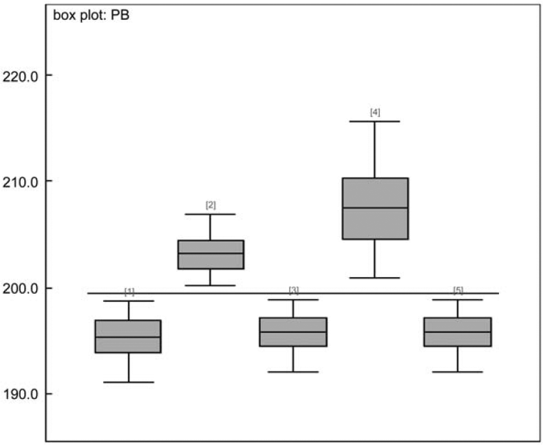
Figure 5 shows the impact of variation in the credibility factor to future premiums for policyholders considered in Table 1. The horizontal line at 200 represents the value of \(\bar{X}\). The box plots represent posterior distributions of \(\hat{P}_i^B\), \(i=1, \ldots, 5\). It gives us a good visual representation of the variability of the premium caused by variation in the credibility factor. The median is shown as a horizontal line within the box. With this information, actuaries can decide whether or not to take an action on the volatility caused by the credibility factor estimation process.

4.4. Disadvantage

The disadvantage of using the proposed Bayesian credibility factor approach shown in Appendices \(A\) and \(B\) is that we drop the subtraction term in Equation (30). The impact of this action is that we systematically shift the prior distribution of \(\hat{a}\) to the right by the amount of \(\hat{v} / n\). However, as seen in Table 4, the resulting Bayesian credibility factors are not materially different from those traditional credibility factors with non-zero values. We believe that it is worthwhile to be biased in the prior distribution of \(\hat{a}\).

Alternatively, we can also use Equations (28) and (33) for a non-negative \(\hat{a}\) to have a more precise prior distribution. Table 6 shows a small sample of trials with this adjustment. We only list trials with relatively large estimates in Table 6, because they contribute relatively large variation in the total squared errors.

5. Remarks

In this article, we have attempted to explore a range of concerns that arise in credibility modeling. As in any statistical estimation problem, the goal is to estimate the value of an unknown quantity, such as a credibility factor or a future premium in the actuarial field. There are different techniques being used for estimation of a credibility factor or a future premium. Nevertheless, the objectives remain the same. We want to use the sample information to estimate the parameters of interest and to assess the reliability of the estimate.

The variability of a credibility estimator \(\hat{Z}\) can cause misclassification of and inaccuracy in the future premium. The benefit of the Bayesian credibility factor approach is that it provides the decision maker an interval estimate of a credibility factor for assessing the accuracy of its point estimator, while the traditional credibility factor approach only provides a point estimator.

Additionally, we use an empirical approach to determine priors for υ and a shown in Appendix B. As described earlier, Bayesian statistical methods not only incorporate available prior information either from experts or previous data, but allow the knowledge in these and subsequent data to accumulate in the determination of the parameter values. To avoid negative estimates of a, we replace Equation (28) with Equation (34). Alternatively, one might consider shrinking Equation (28) for the same purpose. That is, we can consider the shrinkage estimates where we use Equation (28) if it is positive. If Equation (28) is negative, we could replace it with 1/2 of the value from Equation (34). However, it is difficult to say if this will work without further investigation.

When credibility theory is applied to ratemaking, \(\hat{v}\) and \(\hat{a}\),given by Equations (16) and (17), respectively, contain the least information available to the actuary. Even if the components of the prior distributions are not set at their optimal values, the Bayesian credibility factor and the Bayesian credibility premium are still likely to produce better results. Overall, the methodology is easy and straightforward. We believe that this model is a good alternative to credibility modeling.

---

Acknowledgments

The authors gratefully acknowledge the referees for their extensive comments and suggestions that led to significant improvement of the paper. The authors would also like to thank the editors for their help throughout the review process.

          CODE for SIMULATED DATA in [Table 1](292987)
model;
{
### Step 1 ###
  for( i in 1 : 5 ) {
    for( j in 1 : 5 ) {
      y[i , j] ~dnorm(theta[i],tau.v)
    }
  }
for( i in 1 : 5 ) {
    theta[i] ¡ - mu.hat+alpha[i]
  }
### Step 2 ###
  mu.hat ¡ - mean(y[,])
### Step 3 ###
  for( i in 1 : 5 ) {
    alpha[i] ~dnorm(0, tau.a)
  }
### Step 4 ###
  a ~dgamma(2,0.0059)
  tau.a ¡ - 1 / a
### Step 5 ###
  v ~dgamma(10,0.0037)
  tau.v ¡ - 1 / v
### Step 6 ###
  k ¡ - v / a
  z ¡ - 5 / (5 + k)
### Step 7 ###
  for( i in 1 : 5 ) {
    PB[i] ¡- z*mean(y[i,])+(1-z)*mean(y[,])
    }
}