
1. Introduction
Modeling extreme events like the U.S. stock market crash in 1929 and catastrophe insurance losses is certainly a major task for risk managers. In such events, typically, complete information of the underlying distribution is not available. Instead, one has only partial information such as estimates of mean, variance, covariance, or range based on a relatively small sample. Moreover, the sample may contain no extreme observations. While it is almost impossible to obtain accurate tail risk measures based on incomplete information, one can use limited information to compute bounds on the tail risk measures. This paper presents a method to obtain bounds on tail probabilities using only moment information for two kinds of extreme events based on two random variables. These problems are called semiparametric bound problems or generalized Tchebyshev bound problems.
Scarf (1958) applies these ideas in inventory management and Lo (1987) applies them in mathematical finance. Other applications in finance focus on option pricing in the well-known Black and Scholes (1973) setting (Merton 1973; Levy 1985; Ritchken 1985; Boyle and Lin 1997; Bruckner 2007; Schepper and Heijnen 2007) and other asset pricing and portfolio problems (Gallant, Hansen, and Tauchen 1990; Hansen and Jagannathan 1991; Ferson and Siegel 2001, 2003).
The purpose of this paper is to apply the semiparametric bounds approach to estimate the tail probability of joint events which, in many cases, cannot be reliably estimated by traditional statistical methods (e.g., the parametric approach). In particular, our approach is useful in the situations when it is very difficult or inappropriate to make distributional assumptions about random variables of interest, among others, due to scarcity and/or very high volatility of available data. Our approach also aims at tackling the problem of estimating the likelihood of extreme (tail) events for which we have very few observations of outliers. Traditional methods do not work for such tasks because these approaches typically produce a good fit in those regions in which most of the data reside but at the expense of a good fit in the tails (Hsieh 2004).
To address this problem, instead of assuming full knowledge of the distributions of the random variables of interest, we show how to numerically compute upper and lower bounds on the probabilities Pr(X1 ≤ t1 and X2 ≤ t2) and Pr(w1X1 + w2X2 ≤ a) for some appropriate values of t1, t2, w1, w2, a ∈ ℝ, when only second order moment information (means, variances, and covariance) and the support of random variables X1 and X2 are known. Our approach explicitly considers correlations between variables when estimating the bounds. Incorporating variable correlations is important because many models (e.g., models of risk-based capital and enterprise risk management) often involve several random variables, most of which are correlated. For example, let X1 and X2 stand for a random discount factor and a random future insurance payment. If the insurance payment X2 is subject to economic inflation, it will be correlated with the interest rate which determines the discount factor X1. As another example, the variables X1 and X2 can be the returns of two stocks, both of which respond to security market forces.
Following the work of Smith (1990), Cox (1991), Brochett et al. (1995), Zuluaga (2004), Popescu (2005), and Bertsimas and Popescu (2005), we obtain a range of possible values for each of our tail risk measures, corresponding to every distribution that has given moments on a given support. This range can be considered as a 100% confidence interval for the tail risk measure. Generally, semiparametric bounds are robust bounds that any reasonable model must satisfy. It is worth pointing out that the bounds provide “bestcase” estimates and “worst-case” estimates of the probabilities of extreme events. They would be useful for very risk-loving and very risk-averse investors. Moreover, in situations when distributional assumptions can be made, they provide a mechanism for checking the consistency of such assumptions, as well as an initial estimate for cumulative probabilities regardless of any model specifications.
The remainder of the paper is organized as follows. In Section 2, we formally state the semiparametric bound problems considered here and explain the methodology for solving them. Sections 3 and 4 show how the desired semiparametric bounds can be numerically computed with readily available optimization solvers. We present relevant numerical experiments to illustrate the application of our results. In Section 5, we discuss the possible extension of our methodology to obtain bounds when only confidence intervals on moments are given. Section 6 concludes the paper.
2. Preliminaries and notation
For a function φ(x1,x2) of two random variables with joint cumulative distribution function F(X1, X2), its expected value is
EF[ϕ(X1,X2)]=∫Dϕ(X1,X2)dF(x1,x2),
where the set 𝒟 ⊆ ℝ2 is the support of random variables X1 and X2 and ∫𝒟 dF(x1,x2) = 1.
The semiparametric upper bound of given up to second order moment information can be expressed as follows:
ˉp=maxEF[ϕ(X1,X2)] subject to EF(Xi)=μi,i=1,2,EF(X2i)=μ(2)i,i=1,2,EF(X1X2)=μ12,F(x1,x2) a probability distribution on D,
where and are the given first and second order non-central moments of is the given support of the distribution, and denotes the upper bound value. In order to simplify our presentation, let’s assume for the moment that the “point estimates” of the moments of the interested random variables are known. Later, in Section 5, we will show how our results can be adapted in a straightforward fashion to take into account the situation in which confidence intervals rather than point estimates of the moments are known.
The corresponding semiparametric lower bound problem is analogous, except that the objective function is
p_=minEF[ϕ(X1,X2)],
with the same constraints as (2.1).
Notice that from the definitions of and in problems (2.1) and (2.2), the interval is a sharp (or tight) confidence interval on the expected value of for all joint distributions of and with the given moments and support. It follows that for any and the interval is also a confidence interval, although not necessarily sharp. Our aim is to numerically compute useful confidence intervals for relevant choices of the function balancing computational effort and tightness of the confidence interval, using recent advances in optimization.
In particular, given and non-negative random variables and we compute confidence intervals on the probability of the extreme events and by setting and and where is the indicator function of the set Similarly, given we compute confidence intervals on the probability ), by setting and In the second case, we strengthen the bounds in problems (2.1) and (2.2) by adding an additional moment constraint, where That is, we strengthen the bounds by only considering distributions of that can replicate the expected payoff of an exchange option on and This illustrates how additional information can improve the semiparametric bounds. More details are shown in Sections 3 and 4.
The following is the dual of the upper bound problem (2.1) (see, e.g., Karlin and Studden 1966; Bertsimas and Popescu 2002; and Zuluaga and Peña 2005):
ˉd=min(y00+y10μ1+y01μ2+y20μ(2)1+y02μ(2)2+y11μ12) subject to p(x1,x2)≥ϕ(x1,x2) for all (x1,x2)∈D.
The dual of the lower bound problem (2.2) is
d_=max(y00+y10μ1+y01μ2+y20μ(2)1+y02μ(2)2+y11μ12) subject to p(x1,x2)≤ϕ(x1,x2) for all (x1,x2)∈D,
where the quadratic polynomial p(x1,x2) is defined as
p(x1,x2)=y00+y10x1+y01x2+y20x21+y02x22+y11x1x2.
It is not difficult to see that weak duality holds between (2.1) and (2.3), or between (2.2) and (2.4); that is, p ≤ d (or p ≥ d) (Bertsimas and Popescu 2005, Theorem 2.1, p. 785). Furthermore, strong duality holds, i.e., p = d (or p = d), if the following conditions are satisfied (Zuluaga and Peña 2005, Proposition 4.1(ii)):
If problem (2.1) is feasible and there exist y00, y01, y10, y20, y02, y11such that
p(x1,x2)>ϕ(x1,x2), for all (x1,x2)∈D,
then p = d. Similarly, if problem (2.2) is feasible and there exist y00, y01, y10, y20, y02, y11 such that
p(x1,x2)<ϕ(x1,x2), for all (x1,x2)∈D,
then p = d.
Notice that for the two problems to be solved in Sections 3 and 4, is an indicator function bounded on Therefore, the inequality for problem (2.1) holds if we set and for all Similarly, setting and for all the inequality holds for the lower bound problem (2.2). Thus, as long as problem (2.1) or problem (2.2) is feasible when is an indicator function, strong duality (or ) holds. Therefore one can solve (2.3) (or (2.4)) to obtain the desired semiparametric bounds. Before explaining how to solve (2.3) and (2.4), we introduce the following wellknown definition and theorems relevant to the discussion to follow.
Definition 1 (SOS polynomials).
A polynomial
p(x)=p(x1,…,xn)=∑i1,…,in∈Na(i1,…,in)xi11⋯xinn
is said to be a sum of squares (SOS) if
p(x)=∑i[qi(x)]2
for some polynomials
Theorem 1 (Diananda 1962). Let be a quadratic polynomial. If then for all if and only if is an SOS polynomial.
Theorem 1 states that to check if
p(x1,x2)=y00+y10x1+y01x2+y20x21+y02x22+y11x1x2
is positive for all x1,x2 ≥ 0, one can check whether
p(x21,x22)=y00+y10x21+y01x22+y20x41+y02x42+y11x21x22
is an SOS. Here we present Diananda’s Theorem in a form (shown as Theorem 1) that will be suitable for our purposes, instead of presenting it in its original form. Parrilo (2000) and Zuluaga (2004) discuss the equivalence of the original version of Diananda’s Theorem and Theorem 1.
Loosely speaking, in order to solve (2.3), or (2.4), we break the constraint
p(x1,x2)≥( or ≤)ϕ(x1,x2) for all (x1,x2)∈D
into a number of constraints of the form
pi(x1,x2)≥0, for all (x1,x2)∈R+2,i=1,…,m,
where are suitable quadratic polynomials whose coefficients are linear functions of the coefficients of Theorem 1 implies that (2.5) is equivalent to
pi(x21,x22) is an SOS polynomial, i=1,…,m.
As we will show in detail in Sections 3 and 4, this allows us to reformulate problems (2.3) and (2.4) as SOS programs; that is, as an optimization problem, the variables are coefficients of polynomials, the objective is a linear combination of the polynomial coefficients, and the constraints are given by the polynomials being SOS. A detailed discussion about SOS programming is beyond the scope of this article, but the key fact is that these SOS programs can be readily solved by recently developed SOS programming solvers such as SOSTOOLS (Prajna, Papachristodoulou, and Parrilo 2002), GloptiPoly (Henrion and Laserre 2003), or YALMIP (Löfberg 2004). These SOS programming solvers enable us to find the desired bounds on problems (2.1) and (2.2). This approach has been widely used to solve semiparametric bound problems in other areas (see, e.g., Bertsimas and Popescu 2002; Boyle and Lin 1997; and Laserre 2002).
Parrilo (2000) and Todd (2001) show that any SOS program can be reformulated as a semi-definite program (SDP). Specifically, SOS programming solvers work by reformulating an SOS program as an SDP, and then applying SDP solvers such as SeDuMi (Sturm 1999). However, the SDP formulations of SOS programs can be fairly involved. To make it easy to present and reproduce our results, throughout the article we use SOS programming formulations instead of directly reformulating problems (2.1) and (2.2) as SDPs.
3. Extreme probability bounds
In this section, we consider the problem of finding upper and lower bounds on the probability Pr(X1 ≤ t1 and X2 ≤ t2) of two non-negative random variables X1 and X2, attaining values lower than or equal to t1,t2 ∈ ℝ+ respectively, without making any assumption on the distribution of X1 and X2, other than the knowledge of the first and second order moments of their joint distribution (means, variances, and covariance).
3.1. SOS programming formulations
The upper semiparametric bounds for this problem come from problem (2.1) with and and (Section 2):
ˉpExtreme =maxEF[I{X1≤t1 and X2≤t2}] subject to EF(Xi)=μi,i=1,2,EF(X2i)=μ(2)i,i=1,2,EF(X1X2)=μ12,F(x1,x2) a probability distribution on R+2.
Similarly, the lower semiparametric bounds for this problem can be obtained by setting the objective function of problem (2.2) as follows:
p_Extreme =minEF[I{X1≤t1 and X2≤t2}],
with the same constraints as (3.1).
Before obtaining the SOS programming formulation of these problems, let us first examine their feasibility in terms of the moment information. Using Theorem 1 and convex duality (Rockafellar 1970), one can show that problems (3.1) and (3.2) are feasible (i.e., they have solutions), if the moment matrix Σ is a positive definite matrix (i.e., all eigenvalues are greater than zero) and all elements of Σ are greater than zero, where the moment matrix Σ is
Σ=[1μ1μ2μ1μ(2)1μ12μ2μ12μ(2)2].
Now we derive SOS programs to numerically approximate pExtreme and p Extreme with SOS programming solvers.
3.1.1. Upper bound
To derive an SOS program for problem (3.1), we begin by stating its dual explicitly:
ˉdExtreme =min(y00+y10μ1+y01μ2+y20μ(2)1+y02μ(2)2+y11μ12) subject to p(x1,x2)≥I{x1≤t1 and x2≤t2}, for all x1,x2≥0.
To formulate problem (3.3) as an SOS program, we proceed as follows. First notice that the constraint in (3.3) is equivalent to
p(x1,x2)≥1,for all0≤x1≤t1,0≤x2≤t2p(x1,x2)≥0,for allx1,x2≥0.
While the second constraint of (3.4) can be directly reformulated as an SOS constraint using Theorem 1, the first constraint is difficult to reformulate as an SOS constraint. That is, there is no linear transformation from 0 ≤ x1 ≤ t1, 0 ≤ x2 ≤ t2 to ℝ+2 (that would allow us to use Theorem 1). Thus, we change the problem to obtain an SOS program that either exactly or approximately solves problem (3.4). Specifically, consider the following problem related to (3.4):
ˉd′Extreme =min(y00+y10μ1+y01μ2+y20μ(2)1+y02μ(2)2+y11μ12) subject to p(x1,x2)≥1 for all x1≤t1,x2≤t2p(x1,x2)≥0 for all x1≥0,x2≥0.
We relaxed the requirement that x1 and x2 are non-negative in the first constraint. Notice that the constraints in (3.5) are stricter than those in (3.4) since the first constraint of (3.5) includes more values of x1 and x2. Thus, d′Extreme is a (not necessarily sharp) upper bound on d′Extreme; that is, d′Extreme ≥ d′Extreme.
After we apply the substitution x1 → t1 − x1,x2 → t2 − x2 to the first constraint of (3.5), the constraints of (3.5) can be rewritten as
p(t1−x1,t2−x2)−1≥0,for allx1,x2≥0p(x1,x2)≥0,for allx1,x2≥0.
To finish, we apply Theorem 1 to the constraints (3.6) and conclude that (3.5) is equivalent to the following SOS program:
ˉd′Extreme =min(y00+y10μ1+y01μ2+y20μ(2)1+y02μ(2)2+y11μ12) subject to p(t1−x21,t2−x22)−1is an SOS polynomialp(x21,x22)is an SOS polynomial.
The SOS program (3.7) can be readily solved with an SOS programming solver. Thus, if problem (3.1) is feasible, we can numerically obtain a (not necessarily sharp) semiparametric upper bound on the extreme probability, Pr(X1 ≤ t1, X2 ≤ t2) ≤ d′Extreme, by solving problem (3.7) with an SOS solver.
3.1.2. Lower bound
The dual of the lower bound problem (3.2) can be expressed as
d_Extreme =max(y00+y10μ1+y01μ2+y20μ(2)1+y02μ(2)2+y11μ12) subject to p(x1,x2)<π{x1<I1 and x2<I2} for all x1,x2>0
The constraint in problem (3.8) is equivalent to
p(x1,x2)≤1, for all 0≤x1≤t1,0≤x2≤t2p(x1,x2)≤0, for all x1≥t1,x2≥0p(x1,x2)≤0, for all x1≥0,x2≥t2.
Proceeding in the same way as for the upper bound problem, we now change the problem to obtain an SOS program that either exactly or approximately solves problem (3.8). Specifically, consider the following problem related to (3.8):
d_′Extreme =max(y00+y10μ1+y01μ2+y20μ(2)1+y02μ(2)2+y11μ12) subject to p(x1,x2)≤1, for all x1≤t1,x2≤t2p(x1,x2)≤0, for all x1≥t1,x2≥0p(x1,x2)≤0, for all x1≥0,x2≥t2.
Notice that the constraints in (3.10) are stricter than those in (3.8). Thus, d′Extreme is a (not necessarily sharp) lower bound on dExtreme; that is, d′Extreme ≤ d′Extreme
Applying the substitutions x1 → t1 − x1,x2 → t2 − x2 to the first constraint of (3.10) and x1 → t1 + x1,x2 → t2 + x2 to the second and third constraints respectively, it follows that problem (3.10) is equivalent to the following SOS program when Theorem 1 is applied:
d_′Extreme =max(y00+y10μ1+y01μ2+y20μ(2)1+y02μ(2)2+y11μ12) subject to 1−p(t1−x21,t2−x22) is an SOS polynomial −p(t1+x21,x22) is an SOS polynomial −p(x21,t2+x22) is an SOS polynomial.
Following the same route, we can also derive the upper and lower bounds on the joint survival probability Pr(X1 ≥ t1 and X2 ≥ t2) of two nonnegative random variables X1 and X2. The details are shown in Appendix A.
3.2. Example of extreme probability bounds
We select from the NAIC database a major property/casualty insurance company, which we call insurer A. Suppose the insurer faces the problem of managing its risk of unexpectedly high claims and simultaneously unanticipated poor asset returns. This leads insurer A to calculate the bounds on Pr(R ≤ t1, M ≤ t2) given moment information, where ℝ is the company’s return on its invested assets and M is the margin on its insurance business.
The return of asset in insurer A’s portfolio is equal to where and denote the prices of asset at the beginning and the end of the period. Insurer A’s asset portfolio return is the weighted average return of six asset classes: stocks, government bonds, corporate bonds, real estates, mortgages, and short-term investments; that is
R=6∑i=1wiRi=6∑i=1wi(Pi,tPi,t−1−1)=6∑i=1wiPi,tPi,t−1−1=X1−1,
where is the weight of asset class in the portfolio and The following inequalities are equivalent:
R≤t1⟺X1≤t1+1.
We make this shift from asset returns to price ratios to apply our SOS results because we need non-negative random variables.
The margin on the insurance business is defined as
M=1−CR=1−LR−ER,
where CR is the combined ratio, LR is the loss ratio, and ER is the expense ratio.[1] So M is the profit from the underwriting business.
In order to reformulate the condition M ≤ t2 so that the condition fits our SOS results, we replace M ≤ t2 with X2 ≤ t2 + 1 where X2 = M + 1. Using this with (3.12) we get the following:
Pr(R≤t1,M≤t2)=Pr(X1≤t1+1,X2≤t2+1).
The weights wi of different asset categories were calculated from the quarterly data of the National Association of Insurance Commissioners (NAIC). We used the quarterly returns of the Standard & Poor’s 500 (S&P500), the Lehman Brothers intermediate term total return, the domestic high-yield corporate bond total return, the National Association of Real Estate Investment Trusts (NAREIT) total return, the Merrill Lynch mortgage backed securities total return, and the U.S. 30-Day T-Bill as proxies for insurer A’s stock returns, government bond returns, corporate bond returns, real estate returns, mortgage returns and short-term investment returns, respectively. Based on insurer A’s quarterly losses, expenses, and premiums, we calculate the moments of X1 and X2 as follows:
E(X1)=1.0442,E(X21)=1.0967E(X2)=1.1555,E(X22)=1.3715E(X1X2)=1.2086,Cov(X1,X2)=0.0021Var(X1)=0.0063,Var(X2)=0.0364ρ=0.1387.
Insurer A’s average margin on its insurance business (E(M) = 0.1555) is higher than its average asset return (E(R) = 0.0442), while the margin is more volatile (Var(M) > Var(R)). Moreover, the asset return and insurance margin are somewhat positively correlated (0.1387). This implies that occasionally insurer A’s insurance business and investment performances move in the same direction.
Next we compute bounds on the tail probability Pr(R ≤ t1, M ≤ t2) using SOS programming. Then we compare it to the bivariate normal cumulative joint probability with the same moments. The upper left plot in Figure 1 shows the upper bounds of the joint probability Pr(R ≤ t1, M ≤ t2) for different values of t1 and t2, and the upper right one is the corresponding bivariate normal cumulative joint probabilities. Since we are looking at low values of t1 and t2 corresponding to joint extreme events, it is not surprising that our calculated lower bound is zero over this range of their values. The ratios of the upper bounds to the bivariate normal cumulative joint probabilities are shown in the lower graphs.
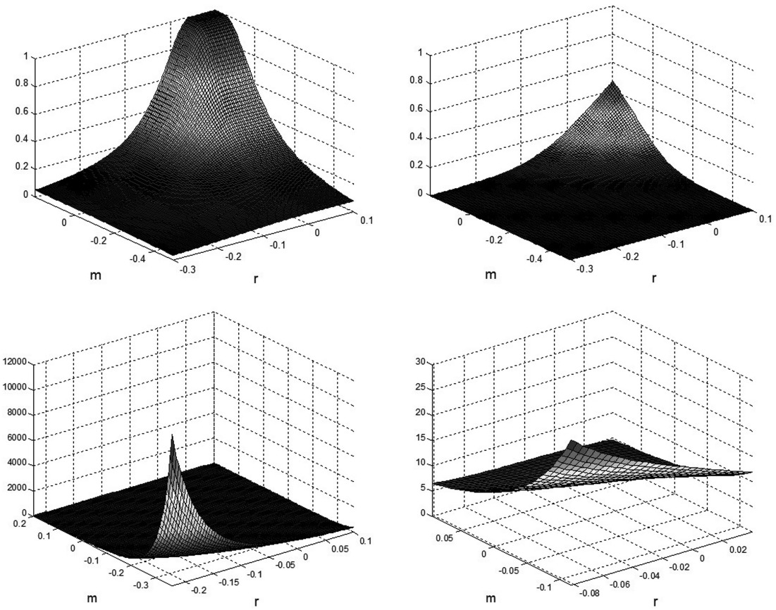
The ratio is large when t1 and t2 are low. For example, consider the event that insurer A has negative investment earnings and simultaneously it has an aggregate loss on its insurance business. In addition to the case with zero investment and insurance returns, this is stated as ℝ ≤ 0, M ≤ 0. From the lower right graph of Figure 1, we see that for t1 = 0 and t2 = 0, the upper bound is about 7.2 times higher than the cumulative joint normal probability. This means that the actual joint distribution may have a much fatter tail than the joint normal distribution. In other words, an extreme event may be more likely to occur than the normal distribution suggests.
4. Value-at-risk probability bounds
Here we find upper and lower bounds on the probability that a portfolio w1X1 + w2X2 (w1, w2 ∈ ℝ+) attains values lower than or equal to a ∈ ℝ, given up to the second order moment information (means, variances, and covariance) on the random variables X1, X2 (X1, X2 ∈ ℝ).
4.1. SOS programming formulations
Finding the sharp upper and lower semiparametric bounds for this problem can be formulated by setting and To obtain tighter bounds (see numerical results in Section 4.2), we include the information of the expected payoff of an exchange option on the assets; that is, we add the moment constraint where ) to illustrate how to incorporate additional information. This is the resulting semiparametric upper bound problem:
ˉpVaR=maxEF[I{w1X1+w2X2≤a}] subject to EF(Xi)=μi,i=1,2,EF(X2i)=μ(2)i,i=1,2,EF(X1X2)=μ12,EF[(X1−X2)+]=γ,F(x1,x2) a probability distribution on R2.
The corresponding lower bound problem has the same constraints as (4.1) and its objective function is
p_VaR=minEF[I{w1X1+w2X2≤a}].
Problems (4.1) and (4.2) have solutions if and only if the moment matrix Σ is a positive semi-definite matrix and pExch < γ < pExch, where pExch and pExch are the upper and lower bounds of problems (2.1) and (2.2) with φ(x1,x2) = (x1 − x2)+, which can be readily computed using SOS techniques (Zuluaga and Peña 2005).
The dual of problem (4.1) is
ˉdVaR=min(y00+y10μ1+y01μ2+y20μ(2)1+y02μ(2)2+y11μ12+y0γ) subject to p(x1,x2)+y0(x1−x2)+≥I{w1x1+w2x2≤a}, for all x1,x2∈R.
Similarly, the dual of problem (4.2) is:
d_VaR=max(y00+y10μ1+y01μ2+y20μ(2)1+y02μ(2)2+y11μ12+y0γ) subject to p(x1,x2)+y0(x1−x2)+≤I{w1x1+w2x2≤a} for all x1,x2∈R.
A straightforward generalization of Proposition 1, and the discussion after Proposition 1, shows that if problems (4.1) and (4.2) are feasible, then pVaR = dVaR and pVaR = dVaR. Thus, if problems (4.1) and (4.2) are feasible, we can solve (4.3) and (4.4) to obtain the desired bounds. Finally, notice that setting y0 = 0 in (4.3) and (4.4) is equivalent to solving the semiparametric bounds (4.1) and (4.2) without using information about the exchange option expected payoff.
4.1.1. Upper bound
The upper bound problem (4.3) is equivalent to
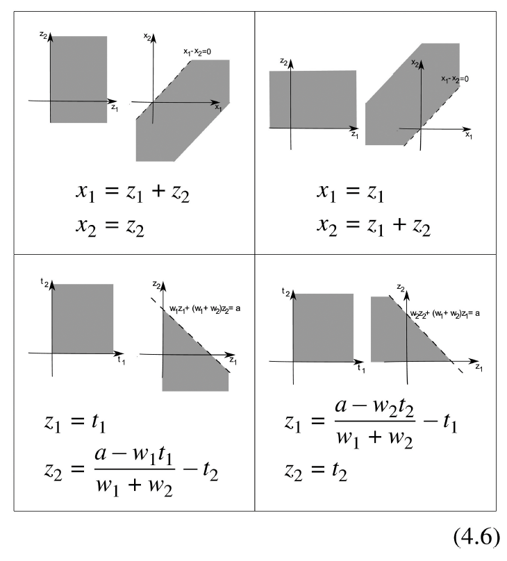
ˉdVaR=min(y00+y10μ1+y01μ2+y20σ21+y02σ22+y11σ12+y0γ) subject to p(x1,x2)+y0(x1−x2)≥1, for all x1,x2 with w1x1+w2x2≤a,x1≥x2p(x1,x2)≥1, for all x1,x2 with w1x1+w2x2≤a,x1≤x2p(x1,x2)+y0(x1−x2)≥0, for all x1,x2 with x1≥x2p(x1,x2)≥0, for all x1,x2 with x1≤x2.
In order to use Theorem 1, we will use the following transformations:

Applying the upper left transformation in (4.6) to the first and third constraints of problem (4.5) and applying the upper right transformation in (4.6) to the second and fourth constraints of problem (4.5), the constraints in (4.5) are equivalent to
p(z1+z2,z2)+y0z1≥1, for all z1,z2withw1(z1+z2)+w2z2≤a,z1≥0p(z1,z1+z2) for all z1,z2withw1z1+w2(z1+z2)≤a,z2≥0p(z1+z2,z2)+y0z1≥0, for all z1,z2withz1≥0p(z1,z1+z2)≥0 for all z1,z2withz2≥0.
Now applying the lower left and right transformations in (4.6) to the first two constraints of (4.7) respectively, these two constraints are equivalent to
p(t1+a−w1t1w1+w2−t2,a−w1t1w1+w2−t2)+y0t1≥1, for all t1≥0,t2≥0p(a−w2t2w1+w2−t1,a−w2t2w1+w2−t1+t2)≥1, for all t1≥0,t2≥0.
Finally, the last two constraints in (4.7) are equivalent to
p(z1+z2,z2)+y0z1≥0, for all z1≥0,z2≥0p(z1−z2,−z2)+y0z1≥0, for all z1≥0,z2≥0p(z1,z1+z2)≥0, for all z1≥0,z2≥0p(−z1,−z1+z2)≥0, for all z1≥0,z2≥0.
After applying Theorem 1, we obtain the SOS formulation for the upper bound of problem (4.3):
ˉdVaR=min(y00+y10μ1+y01μ2+y20σ21+y02σ22+y11σ12+y0γ)
subject to the following being SOS polynomials:
p(t21+a−w1t21w1+w2−t22,a−w1t21w1+w2−t22)+y0t21−1p(a−w2t22w1+w2−t21,a−w2t22w1+w2−t21+t22)−1p(z21+z22,z22)+y0z21p(z21−z22,−z22)+y0z21p(z21,z21+z22)p(−z21,−z21+z22).
4.1.2. Lower bound
The lower bound problem (4.4) is equivalent to
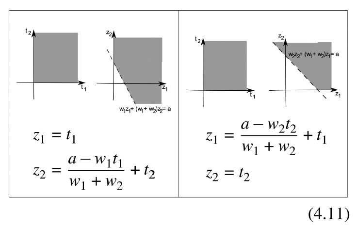
d_VaR=max(y00+y10μ1+y01μ2+y20σ21+y02σ22+y11σ12+y0γ) subject to p(x1,x2)+y0(x1−x2)≤1, for all x1,x2 with x1≥x2p(x1,x2)≤1, for all x1,x2 with x1≤x2p(x1,x2)+y0(x1−x2)≤0, for all x1,x2 with w1x1+w2x2≤a,x1≥x2p(x1,x2)≤0, for all x1,x2 with w1x1+w2x2≤a,x1≤x2
Here we will use the following extra transformations:

Following steps analogous to those taken in Section 4.1.1 for problem (4.5), we obtain that problem (4.4) is equivalent to
d_VaR=max(y00+y10μ1+y01μ2+y20σ21+y02σ22+y11σ12+y0γ)
subject to the following being SOS polynomials:
1−p(z21+z22,z22)−y0z211−p(z21−z22,−z22)−y0z211−p(z21,z21+z22)1−p(−z21,−z21+z22)−p(t21+a−w1t21w1+w2+t22,a−w1t21w1+w2+t22)−y0t21−p(a−w2t22w1+w2+t21,a−w2t22w1+w2+t21+t22).
4.2. Example of value-at-risk probability bounds
Given a specified tail probability β, the weights w1 and w2, as well as the moment information on X1 and X2, the value-at-risk (VaR) bound problem finds the upper and lower bounds on a where Pr(w1X1 + w2X2 ≤ a) = β. To solve this problem, we find bounds on Pr(w1X1 + w2X2 ≤ a) for different values of a and then solve the inverse problem for bounds on a given β.
We first calculate the semiparametric VaR probability bounds given only the mean, variance, and covariance of the two components of the portfolio. Then we add one more constraint that the expected value of the exchange option between and must equal The following example shows that the VaR bounds with exchange option information are tighter since we add more constraints to the optimization.
We analyze a portfolio investing in the S&P 500 Index and the Dow Jones U.S. Small-Cap Index. Suppose we invest 1/3 of our assets in the S&P 500 Index, 1/3 in the Dow Jones U.S. Small-Cap Index, and 1/3 in a risk-free fund paying a flat 0.01 percent per day. Thus, our portfolio daily return is (1/3)X1 + (1/3)X2 + (1/3)0.01.
The moments are based on the daily historical log-returns from February 24, 2000 to October 24, 2007. There are 1,923 observations in our sample. Let and be the log-return of the S&P 500 Index and Dow Jones U.S. SmallCap Index in percentage per day for day ). Their moments are as follows:
E(X1)=0.0059,E(X21)=1.2158E(X2)=−0.2117,E(X22)=112.8609E(X1X2)=1.4161,Cov(X1,X2)=1.41736Var(X1)=1.2158,Var(X2)=112.8160ρ=0.1210,E((X1−X2)+)=0.4464.
Apparently, the Dow Jones U.S. Small-Cap Index is much more volatile than the S&P 500 (112.8160 percent vs. 1.2158 percent).
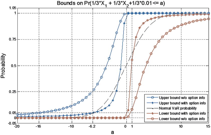
We now calculate the upper and lower bounds for the probability when the portfolio return falls below a given level a, i.e.,
Pr((1/3)X1+(1/3)X2+(1/3)0.01≤a).
The corresponding bounds are shown in Figure 2. The lines with –o-- represent the upper and lower bounds on the VaR probability, without using the exchange option information. These bounds are obtained by setting y0 = 0 in Equations (4.9) and (4.12). The lines with represent the upper and lower bounds on the VaR probability, using the exchange option information. Obviously the exchange option information tightens the VaR probability bounds significantly. These semiparametric upper and lower bounds apply to all possible joint probabilities, including the bivariate normal joint probability. The VaR probability corresponding to a normal distribution with the same first and second order moments is drawn with the broken line in the middle. Interestingly, the normal VaR probability lies outside the tighter bounds using the exchange option information. This means that the normal model does not satisfy the constraint

Here we use the VaR probability bounds in Figure 2 to obtain the upper and lower bounds of the VaR itself, with and without the exchange option price constraint. Figure 2 gives us an idea of how likely the return of this portfolio will be lower than a in 1 day under different conditions. Consider a 5% VaR. We look at the horizontal line through the 0.05 level on the vertical axis—it intersects the –o-- curves at a values of −16 and 1. The best we can say is that
−16%<VaR0.05<1%
per day. Then reading the curves with the exchange option information we find that
−6.2%<VaR0.05<0%
per day. Clearly the additional information greatly improves our knowledge of future possible outcomes.
5. Semiparametric bounds given confidence intervals on moments
Thus far in this paper we have assumed that the moments information is given in the form of point estimates of the moments of the random variables of interest. In practice, it is typical to have not only a point estimate but also a confidence interval estimate on a moment, which provides information about the accuracy of the point estimate. Therefore, an important question is how to adapt the results presented so far in order to handle the situation in which the moment information is given in the form of confidence intervals on the moments. To answer this question, consider the following general upper semiparametric bound problem:
max{EF[ϕ(X1,…,Xn)]} subject to EF[fj(X1,…,Xn)]=σj,j=1,…,m,F(x1,…,xn) a probability distribution on D⊆Rn,
where represent the moments. Assume now that instead of knowing the point estimates of the moments, we have an estimate of the moments in the form of confidence intervals. Loosely speaking, assume that the estimates are given in the form where is the point estimate. With these estimates, one can compute a confidence interval on the expected value of over all distributions of the random variables with moments within the confidence intervals by solving the problem
max{EF[ϕ(X1,…,Xn)]} subject to ˆσ−j≤EF[fj(X1,…,Xn)]≤ˆσ+j,j=1,…,m,F(x1,…,xn) a probability distribution on D⊆Rn.
Using the same duality arguments discussed in Section 2, under suitable conditions (similar to Proposition 1), the objective value of the problem above can be found by solving the following dual problem:
min{y0+m∑j=1(y+jˆσ+j−y−jˆσ−j)}subject to y0+m∑j=1(y+j−y−j)fj(x1,…,xn)≥ϕ(x1,…,xn) for all (x1,…,xn)∈D,y+j,y−j∈R+,j=1,…,m,y0∈R.
Note that the dual of the original problem (5.1) is:
min{y0+∑mj=1yjσj} subject to y0+∑mj=1yjfj(x1,…,xn)≥ϕ(x1,…,xn) for all (x1,…,xn)∈Dyj∈R,j=0,…,m.
In both problems (5.3) and (5.4), the objective function is linear, and all the constraints are linear except for the first constraint of the problem. In fact, the difficulty of solving any of these problems comes from the first constraint, which is the “same” for both problems. For the particular semiparametric bound problems we have considered here, we have shown how to address this first constraint using SOS techniques. Because the difference between these two problems is the addition of extra variables that are linear in the objective and in the extra constraints, having an SOS formulation for the original problem given point estimates of moments means that an SOS formulation for the problem with confidence intervals on moments can be obtained in straightforward fashion by accordingly changing the objective of the SOS formulation of the original problem, and adding the adequate linear constraints. The resulting SOS formulation can then be efficiently solved using SOS optimization softwares such as SOSTOOLS. As an example, the SOS formulation (3.5) to obtain a semiparametric upper bound for the extreme probability Pr(X1 ≤ t1 and X2 ≤ t2) can be modified as follows, in order to consider the situation in which only the confidence intervals on the moments are available:
min(y00+y+10μ+1+y+01μ+2+y+20μ(2)+1+y+02μ(2)+2+y+11μ+12−y−10μ−1−y−01μ−2−y−20μ(2)−1−y−02μ(2)−2−y−11μ−12)subject to p(t1−x21,t2−x22)−1 is an SOS polynomial, p(x21,x22) is an SOS polynomial, y+10,y−10,y+01,y−01,y+20,y−20,y+02,y−02,y+11,y−11∈R+,y00∈R.
Above, the {·}+ and {·}− in the moments, represent the upper and lower bounds of the confidence interval used to estimate the moments. Similar straightforward modifications can be made for all the SOS formulations of semiparametric bound problems considered in the paper.
It is important to note that in our discussion above we have assumed that the confidence intervals have been obtained independently for each moment. Developing SOS formulations for relevant semiparametric bound problems considering more complex (dependent) confidence intervals will be the topic of future work.
6. Conclusions
In this paper, we have illustrated a new optimization technique known as sum of squares (SOS) programming to find optimal bounds for the probability of extreme events involving two random variables, given only the first and second order moment information. An interesting aspect is that we work solely under the physical measure. This avoids the difficulty of estimating moments of the risk-neutral distribution.
We extend the application of classical moment problems (or semiparametric methods) to finance, insurance, and actuarial science by examining two extreme probability problems, both taking into account correlations between random variables. The first problem allows us to put “100% confidence intervals” on the probability of joint extreme events. The second finds VaR probability bounds on the sum of two variables, given up-to-the-second moment information. In each case the moment information is given by point estimates, which are based on historical observations or judgments from scenario analysis. We provide the examples to illustrate the potential usefulness of moment methods in assessing probability of rare events. We also show that the proposed method can be modified in a straight-forward fashion to obtain semiparametric bounds based on confidence intervals rather than point estimates of the moments.
There are other applications where our approach could be useful. For example, this approach can be used to estimate the default probability of fixed-income securities where incomplete knowledge on the enterprise and economic factors drives the credit risk. In other areas such as inventory and supply chain management, this approach can be applied to find inventory policies that will be applicable to different (unknown) demand distributions in the future. Even when the distributions of the random variables are assumed to be known, this approach can be implemented to measure sensitivity of a joint probability, VaR, or other variables to model misspecification as in Lo (1987) and Hobson, Laurence, and Wang (2005).
Some important issues for future research clearly deserve more investigation. For example, it will be interesting to analyze the bounds on tail distribution given the moments of extreme values instead of the moments of the whole distribution. A further question involves to what extent our results would change if we incorporate distribution class information (e.g., continuous, symmetric, unimodal, etc.) in our bound problems. We leave these questions for future research.
_._the_left_and_right_g.png)