Risk Aggregation: A General Approach via the Class of Generalized Gamma Convolutions

1. Introduction

Risk aggregation is of fundamental importance for insurance. This is because risk aggregation is in fact a precursor of risk pooling, a principle that is seen by some as the insurance’s reason d’etre. To see how crucial risk aggregation is for risk pooling, consider a group of n ∈ N individuals (also, business lines, risk components in a portfolio of risks, etc.), where each one of i ∈ {1, . . . , n} faces a risk represented by the random variable (RV) X_i, then a sharing rule Y(X₁, . . . , X_n) is called risk pooling if it is a function of the aggregate risk X₁ + . . . + X_n, only, that is Y(X₁, . . . , X_n) = Y(X₁ + . . . + X_n) (e.g., Aase 2004 for details). Hence, it is clear that to reap the benefits of risk pooling, insurers must study and understand risk aggregation thoroughly. From now and on, X₁, . . . , X_n stand for insurance risk RVs, and X₁ + . . . + X_n ≔ S_n denotes the associated aggregate risk.

Specific examples of risk aggregation are naturally abundant in all areas of insurance business. For classical applications, one has to go no further than the renowned individual (e.g., Dhaene and Vincke 2004) and collective (e.g., Goovaerts 2004) risk models. Specifically, in the case of the individual risk models (IRMs), for a fixed n as hitherto and independent but not identically distributed risk RVs X₁, . . . , X_n, the aggregate risk is as before denoted by S_n. Also, in the case of the collective risk models (CRMs), the number of risks, denoted by N is assumed random and independent of identically distributed and mutually independent (IID) RVs X₁, . . . , X_N; the aggregate risk is then denoted by S_N ≔ X₁ + . . . + X_N.

In order to comprehend the implications of risk aggregation, and merely comply with the norms of the risk informed decision making, insurers are concerned with the stochastic properties of the RVs S_n and S_N, that is, with the corresponding cumulative distribution functions (CDFs). Whether the IRM or CRM are considered, it is often tempting to approximate these CDFs with the use of the Lindeberg–Lévy central limit theorem (CLT). To this end, arguments like (i) the number of risks is large, (ii) the risks are not too heterogeneous, and (iii) the distributions of the risk RVs are not too skewed are quite common. Unfortunately, none of the above must be true in reality. Furthermore, statements (ii) and (iii) are often violated as insurance risk RVs due to distinct risk sources can be very unalike, and, as a rule, positively skewed. Another problem with the aforementioned variant of the CLT is that there are situations (not rare) where the risk RVs of interest have infinite second moments (e.g., Seal 1980 and references therein). We refer to Brockett (1983) and references therein for some interesting examples of how the CLT is misused in insurance applications.

The standard CLT-based approximation of the aggregate risk’s CDF, a.k.a. the normal approximation (NA), can be considered a moment matching approximation (MMA) that hinges on the first two moments only. A generalization of NA that incorporates skewness is the so-called normal-power (NP) approximation (e.g., Ramsay 1991). An alternative approach to count for skewness that is of great popularity among practicing actuaries is the shifted-gamma approximation (SGA), which aims to match the first three moments (Hardy 2004). Clearly, the choice of how many moments to match is somewhat ad hoc. Thus, more general approximations that aim at matching an arbitrary number of moments have been proposed (e.g., Cossette et al. 2016 for a recent reference).

Admittedly, MMAs, both the ones mentioned above and others alike, are convenient and intuitive to convey to upper management, yet rather problematic. For instance, even the two moments-based NA method requires finite second moments, and it is inapplicable otherwise. The approach of Cossette et al. (2016) achieves better accuracy at the price of requiring the finiteness of higher order moments. In addition, in the latter case, the method is often rather computationally intensive.

In this paper, we put forward a new efficient method to approximate the CDFs of the aggregate risk RVs S_n and S_N. Our approach approximates the CDFs of interest to any desired precision, works equally well for light- and heavy-tailed CDFs and is reasonably fast, irrespective of the number of summands. We organize the rest of this paper as follows: Section 2 provides a high-level overview of our approach, and Sections 3, 4, and 5 explain in detail its three main pillars, which are, respectively, the class of Padé approximations, the family of generalized gamma convolutions, and the Gaver-Stehfest algorithm. The theory we propose is then elucidated by a variety of practical examples borrowed from Bahnemann (2015). More specifically, in Section 6 we demonstrate the effectiveness of the new MMA in the context of stand-alone risk RVs first and then in the context of aggregate risk RVs with and without policy modifications.

2. Brief description of the method

In order to outline the essence of our proposed technique in the simplest possible manner, in this section we consider the framework of the IRM; however, the ideas are equally applicable in the context of the CRM (Section 6 of this paper). Let \(X_1, \ldots, X_n\) be positive and mutually independent RVs with arbitrary corresponding CDFs \(F_1, \ldots, F_n\). Also denote by \(\phi_i(z):=\mathbb{E}\left[\exp \left(-z X_i\right)\right]\) the Laplace transform (LT) of the RV \(X_i, i=1, \ldots, n\). Our goal is to approximate the CDF \(F\) of the aggregate RV \(S=X_1+\cdots+X_n\).

Let \(\phi(z):=\mathbb{E}[\exp (-z S)](\) also, \(\mathcal{L}(z))\) denote the LT of the aggregate risk RV S, then we readily have

\[ \phi(z)=\prod_{i=1}^{n} \phi_{i}(z) \tag{1} \]

and

\[ F(x)=\mathcal{L}^{-1}\left\{\frac{\phi(z)}{z}\right\}(x), \quad x \geq 0 .\tag{2} \]

Hence, by combining (1) and (2), we are able to obtain the desired approximation of the CDF \(F\) given that there exist reliable methods to: (i) approximate each LT \(\phi_i(z)\), and (ii) invert LTs. Next in Sections 3-5, we demonstrate that (i) and (ii) can be achieved very successfully. Namely, in Section 3, we approximate the Laplace transform \(\phi_i\) with the help of the Laplace transform of certain gamma convolutions, and we utilize the machinery of Padé approximations to determine the involved shape and rate parameters. In Section 4, we reintroduce the family of generalized gamma convolutions, and, finally, in Section 5, we briefly explain the Gaver-Stehfest method to invert Laplace transforms. The proposed MMA may at the first glance seem complex, but when implemented it is utterly user-friendly and requires minimal human involvement.

3. Padé approximations

To start off, we note that (1) requires approximating the LT of the RV \(X_i\) (the CDF of the RV \(X_i\) is then established via (2)). We accomplish this with the help of \(m\)-fold convolutions of gamma-distributed RVs, succinctly \(\Gamma_i \sim {Gamma}\left(\alpha_i, \beta_i\right), i=1, \ldots, m\). In other words, we seek to choose the parameters \(\left\{\alpha_i\right\}_{1 \leq i \leq m}\) and \(\left\{\beta_i\right\}_{1 \leq i \leq m}\), so that the CDF of the approximant of order \(m \mathrm{RV} \tilde{X}_{i,(m)}:=\sum_{i=1}^m \Gamma_i\) is close in an appropriate sense to the CDF of the \(\mathrm{RV} X_i i=1, \ldots, n\). In the rest of the paper, we omit the subscript ( \(m\) ) whenever the order of the approximation is fixed. Also, for the sake of the expositional simplicity of the discussion in the present section, and sometimes thereafter, we omit the subscript \(i\) and write \(X\) instead of \(X_i\), and \(\phi\) instead of \(\phi_i\).

In terms of LTs, we seek to choose the parameters \(\left\{\alpha_i\right\}_{1 \leq i \leq m}\) and \(\left\{\beta_i\right\}_{1 \leq i \leq m}\), so that the approximant LT

\[ \tilde{\phi}(z):=\mathbb{E}\left[\exp \left(-z \sum_{i=1}^{m} \Gamma_{i}\right)\right]=\prod_{i=1}^{m}\left(1+z / \beta_{i}\right)^{-\alpha_{i}} \]

is close to the function \(\phi(z)=\mathbb{E}[\exp (-z X)]\). Our method is essentially an MMA. Note that the moments of \(X\) can be computed as \(\mathbb{E}\left[X^k\right]=(-1)^n \phi^{(k)}(0)\), thus matching the first \(m\) moments of \(\tilde{X}\) and \(X\) is equivalent to matching the derivatives (of order \(k=1,2, \ldots, m\) ) of \(\tilde{\phi}\) and \(\phi\) at \(z=0\). However, our approach allows for a number of important improvements.

Note 1. A significant innovation of our method is that we match the derivatives of \(\tilde{\phi}\) and \(\phi\) not at \(z=0\) but at some point \(z=z^*>0\). This is crucial if we want our technique to be applicable to risk RVs with heavy tails, for which the moments (and thus the derivatives \(\left.\phi^{(k)}(0)\right)\) may fail to exist. If the risk RV X has exponentially light tails, we may as well choose \(z^*=0\), but in general z* must be strictly positive.

Note 2. Another distinguishing feature of our approach is that \(\tilde{\phi}\) converges to \(\phi\) uniformly and exponentially fast, and in particular the approximant \(R V \tilde{X}\) converges in distribution to the RV X.

Note 3. Our method requires \(2 m\) parameters (unique up to permutation) to match the first \(2 m\) moments of the RVs \(\tilde{X}\) and \(X\). As at least \(2 m\) parameters are required to complete this task, the method we put forward herein is optimal in this sense.

3.1. Approximation of order two

In order to explain the main ideas behind our algorithm, let us consider a simple case where m = 2 and z* = 1. In this case the problem reduces to the following one: we want to find four positive numbers \(\alpha_1\), \(\alpha_2\), \(\beta_1\) and \(\beta_2\) such that the derivatives of the LT φ at z = 1 coincide with derivatives of the approximant LT

\[ \tilde{\phi}_{(2)}(z)=\left(1+z / \beta_{1}\right)^{-\alpha_{1}}\left(1+z / \beta_{2}\right)^{-\alpha_{2}} \]

also at point z = 1. In order to compute the four constants \(\alpha_1\), \(\alpha_2\), \(\beta_1\) and \(\beta_2\) we need to have at least four equations, so now we need to solve the following system

\[ \begin{aligned} \left.\frac{d^{k}}{d z^{k}}\left(1+z / \beta_{1}\right)^{-\alpha_{1}}\left(1+z / \beta_{2}\right)^{-\alpha_{2}}\right|_{z=1} & =\phi^{(k)}(1) \\ & k \in\{1,2,3,4\}. \end{aligned} \tag{3} \]

If we were to compute the derivatives in the left-hand side of (3) and then to simplify the resulting equations, we would have obtained a fairly complicated system of four nonlinear equations in \(\alpha_1\), \(\alpha_2\), \(\beta_1\) and \(\beta_2\). However, analyzing these equations theoretically would not be feasible due to their complexity and even solving them numerically would be a major problem.

In order to avoid the complexity, we take logarithms before differentiating. Thus, instead of matching the derivatives \(\phi^{(k)}\) and \(\tilde{\phi}_{(2)}^{(k)}\) for \(k=1,2,3,4\), we match the derivatives of \(\ln (\phi(z))\) and \(\ln \left(\tilde{\phi}_{(2)}(z)\right)\) of order \(k=1,2,3,4\). The end result is clearly the same, but computing \(\alpha_1\), \(\alpha_2\), \(\beta_1\) and \(\beta_2\) is much simpler, as we demonstrate in a moment. With this change, the system of four equations for finding \(\alpha_1\), \(\alpha_2\), \(\beta_1\) and \(\beta_2\) looks as follows:

\[ \begin{array}{l} \left.\frac{d^{k}}{d z^{k}} \ln \left[\left(1+z / \beta_{1}\right)^{-\alpha_{1}}\left(1+z / \beta_{2}\right)^{-\alpha_{2}}\right]\right|_{z=1} \\ \quad=\left.\frac{d^{k}}{d z^{k}} \ln [\phi(z)]\right|_{z=1}, \quad k \in\{1,2,3,4\} . \end{array} \tag{4} \]

Let us denote \(s_{k}:=-\left.(1 / k!) \frac{d^{k+1}}{d z^{k+1}} \ln [\phi(z)]\right|_{z=1}\). As we see later, it is easy to compute s_k numerically in each case of interest, thus for now we treat these numbers as known quantities. Computing the derivatives in the left-hand side of (4), we obtain a system of four equations

\[ \begin{array}{l} \frac{\alpha_{1}}{\left(1+\beta_{1}\right)^{k}}+\frac{\alpha_{2}}{\left(1+\beta_{2}\right)^{k}}+\frac{\alpha_{2}}{\left(1+\beta_{2}\right)^{k}}+\frac{\alpha_{2}}{\left(1+\beta_{2}\right)^{k}} \\ \quad=(-1)^{k} s_{k-1}, \quad k \in\{1,2,3,4\}. \end{array} \tag{5} \]

At this stage, that is in order to solve the nonlinear equations in (5) and find \(\alpha_1\), \(\alpha_2\), \(\beta_1\) and \(\beta_2\), we employ the toolbox of Padé approximations.

Namely, we introduce yet another function ψ(z) ≔ −φ′(z)/φ(z). Then system (4) is equivalent to

\[ \left.\frac{d^{k}}{d z^{k}}\left[\frac{\alpha_{1}}{z+\beta_{1}}+\frac{\alpha_{2}}{z+\beta_{2}}\right]\right|_{z=1}=\psi^{(k)}(1), \quad k \in\{0,1,2,3\} . \tag{6} \]

Note that we can write

\[ \frac{\alpha_{1}}{z+\beta_{1}}+\frac{\alpha_{2}}{z+\beta_{2}}=\frac{A+B(z-1)}{1+C(z-1)+D(z-1)^{2}} \tag{7} \]

for some constants A, B, C and D. Now we can express system of four equations (6) in an equivalent way by saying that the first four terms of the Maclaurin expansion of the rational function

\[ \frac{P(w)}{Q(w)}:=\frac{A+B w}{1+C w+D w^{2}} \]

must match the corresponding terms of the Maclaurin expansion

\[ \psi(1+w)=s_{0}+s_{1} w+s_{2} w^{2}+s_{3} w^{3}+\ldots, \]

in other words we have a single equation

\[ \begin{aligned} \frac{A+B w}{1+C w+D w^{2}}=s_{0}+s_{1} w+s_{2} w^{2}+s_{3} w^{3}+O\left(w^{4}\right) & , \\ w & \rightarrow 0, \end{aligned} \tag{8} \]

(note that we have introduced here a new variable w ≔ z − 1). Equation (8) tells us that the rational function P(w)/Q(w) is a [1/2] Padé approximation to the function ψ(1 + w). In general, a [p/q] Padé approximation to a function f is a rational function P(w)/Q(w) (with deg(P) = p and deg(Q) = q) that has the same first p + q + 1 terms in Maclaurin expansion as the function f(w).

It turns out that single equation (8) contains all the information necessary for finding the constants A, B, C and D. By multiplying both sides of equation (8) by Q (w) = 1 + Cw + Dw² we obtain

\[ \begin{aligned} A+B w= & \left(1+C w+D w^{2}\right) \\ & \left(s_{0}+s_{1} w+s_{2} w^{2}+s_{3} w^{3}+O\left(w^{4}\right)\right), \\ & w \rightarrow 0 . \end{aligned} \tag{9} \]

Identifying the coefficients in front of powers of w in both sides of the above equation we obtain a system of four linear (!) equations

\[ \left\{\begin{array}{l} A=s_{0}, \\ B=C s_{0}+s_{1}, \\ 0=D s_{0}+C s_{1}+s_{2}, \\ 0=D s_{1}+C s_{2}+s_{3}. \end{array}\right. \tag{10} \]

Note that this system of four linear equations can be solved very easily by first finding C and D from the third and fourth equations, and then substituting these results into the first and second equations would give us the values of A and B.

Now that we have found A, B, C, and D, and so we can compute \(\beta_1\) and \(\beta_2\) by noting that

\[ \left(1+\beta_{1}+w\right)\left(1+\beta_{2}+w\right)=1+C w+D w^{2}, \]

and then the constants \(\alpha_1\) and \(\alpha_2\) can be found by the formula

\[ \alpha_{i}=\frac{P\left(-1-\beta_{i}\right)}{Q^{\prime}\left(-1-\beta_{i}\right)}=\left.\frac{A+B w}{C+2 D w}\right|_{w=-1-\beta_{i}.} \]

Remarkably, all we have done so far is the partial fraction decomposition for the rational function P(w)/Q(w) as in (7). This process, which can be done by hand, has provided us with the desired constants \(\alpha_1\), \(\alpha_2\), \(\beta_1\) and \(\beta_2\), and so with the approximant LT φ̃₍₂₎.

3.2. Extension to the approximation of any order

To generalize the method described in the previous subsection to arbitrary orders m and arbitrary choice z*, we follow the same steps and arrive at the problem of finding [m − 1/m] Padé approximant to the function ψ(z* + w), that is, instead of (7) and (8) we have

\[ \begin{aligned} \sum_{i=1}^{m} \frac{\alpha_{i}}{z^{*}+\beta_{i}+w}= & \frac{a_{0}+a_{1} w+\cdots+a_{m-1} w^{m-1}}{1+b_{1} w+b_{2} w^{2}+\cdots+b_{m} w^{m}} \\ = & s_{0}+s_{1} w+s_{2} w^{2}+\cdots \\ & +s_{2 m-1} w^{2 m-1}+O\left(w^{2 m}\right), \end{aligned} \tag{11} \]

where \(s_k:=(1 / k!) \Psi^{(k)}\left(z^*\right)\). This allows us to find the coefficients \(b_i, a_i\) by solving a system of linear equations similar to (10) and then to obtain the required numbers \(\left\{\alpha_i\right\}_{1 \leq i \leq m}\) and \(\left\{\beta_i\right\}_{1 \leq i \leq m}\) by doing the partial fraction decomposition in (11).

The main input for this algorithm is the sequence of coefficients \(s_k=(1 / k!) \Psi^{(k)}\left(z^*\right)\). These coefficients are typically not available in closed form, but they can be easily computed numerically. Indeed, we first compute the numbers

\[ g_{k}:=\phi^{(k)}\left(z^{*}\right)=(-1)^{k} \int_{0}^{\infty} x^{k} e^{-z^{*} x} \mathrm{~d} F(x), \quad k \geq 0, \tag{12} \]

to a high precision by a numerical quadrature (the double-exponential quadrature of Takahasi and Mori (1974) is particularly well suited for such calculations). Next we observe that

\[ \frac{d}{d z} \phi(z)=-\psi(z) \phi(z). \tag{13} \]

Rewriting this identity in terms of Taylor series centred at z* gives us

\[ \begin{aligned} \sum_{k \geq 0} g_{k+1}\left(z-z^{*}\right)^{k} / k! & =-\left(\sum_{n \geq 0} s_{n}\left(z-z^{*}\right)^{n}\right) \\ & \times\left(\sum_{k \geq 0} g_{k}\left(z-z^{*}\right)^{k} / k!\right) . \end{aligned} \]

Comparing the constant term in the Taylor series in the left-hand side and the right-hand side of the above equation we find that s₀ = −g₁/g₀, and comparing the coefficients in front of (z − z*)^k gives us

\[ s_{k}=-\frac{1}{g_{0}}\left(\frac{g_{k+1}}{k!}+\sum_{i=0}^{k-1} s_{i} \frac{g_{k-i}}{(k-i)!}\right), \tag{14} \]

which allows to compute s_k recursively for all k ≥ 1.

3.3. A simple numerical example and a question arising from it

To illustrate our method on a numerical example of actuarial interest, let us assume that X is distributed Weibull with the probability density function (PDF)

\[ f(x)=(3 / 4) x^{-1 / 4} \exp \left(-x^{-3 / 4}\right), \quad x \geq 0 . \]

Weibull distribution has been frequently chosen to model insurance risks (Mikosch 2009; Klugman, Panjer, and Willmot 2012 for general discussions).

We fix m = 2 and z* = 1; by computing numerically the integral in (12) we calculate

\[ \begin{array}{c} g_{0} \approx 0.5193711, g_{1} \approx-0.2123717, g_{2} \approx 0.2179689, \\ g_{3} \approx-0.3665409, g_{4} \approx 0.8649004 . \end{array} \]

Then we use (14) to find

\[ \begin{array}{l} s_{1} \approx 0.4089017, s_{2} \approx-0.252478, \\ s_{3} \approx 0.1638276, s_{4} \approx-0.1094817 \end{array} \]

and solving system of linear equations (10) we obtain

\[ \begin{array}{l} A \approx 0.4089017, B \approx 0.1766115, \\ C \approx 1.0493709, D \approx 0.2472855 . \end{array} \]

The polynomial \(Q(w)=1+C w+D w^2\) has two roots \(\approx\) -2.7985663 and \(\approx-1.4449925\), thus we find \(\beta_1 \approx\) 1.79856636 and \(\beta_2 \approx 0.4449925\). Using the formula \(\alpha_i=P\left(-1-\beta_i\right) / Q^{\prime}\left(-1-\beta_i\right)\) we find \(\alpha_1 \approx 0.25501185\) and \(\alpha_2 \approx 0.4591888\). Thus we have found an approximation to the Weibull distribution of interest. Namely, we have approximated \(X\) with the help of \(\tilde{X}_{(2)}\), such that the latter RV is equal in distribution to \(\Gamma_1+\Gamma_2\), with \(\Gamma_i \sim \operatorname{Gamma}\left(\alpha_i, \beta_i\right), i=1,2\).

We conclude this section with an important observation, which paves the path to the introduction of the class of GGCs latter on in the next section. Namely, let the RV X be distributed Weibull with the following PDF (the shape parameter is now greater than one)

\[ f(x)=(3 / 2) x^{1 / 2} \exp \left(-x^{3 / 2}\right), \quad x \geq 0 . \]

For this setup, we find that \(\beta_1 \approx 2.58-1.37 i\) and \(\beta_2 \approx 2.58+1.37 i\) do not belong to \((0, \infty)\), which shows that our algorithm does not always give a legitimate approximation in the form \(\Gamma_1+\Gamma_2\), with \(\Gamma_i \sim \operatorname{Gamma}\left(\alpha_i, \beta_i\right)\). This outcome is rather unfortunate, but similar inconveniences have been encountered in the context of other MMAs (e.g., Cossette et al. 2016).

This raises an important question:

Does there exist a (rich) class of CDFs for which the Padé approximations described above always yield meaningful results?

In the next section we show that the answer to this question is in affirmative, and we also discuss the convergence of our refined MMA method.

4. Generalized gamma convolutions

The class of Generalized Gamma Convolutions comprises distributions which are weak limits of the RVs of the form \(\sum_{i=1}^m \Gamma_i\), where \(\Gamma_i \sim \operatorname{Gamma}\left(\alpha_i, \beta_i\right)\) and \(\alpha_i>0, \beta_i>0, i=1, \ldots, m\). It seems that GGCs were first used by Thorin in 1977, who employed their properties to prove that the log-normal distribution is infinitely divisible (e.g., Bondesson 1992 for an excellent discussion).

The most convenient way to describe the class of GGCs is via LTs. Note that for a RV \(\sum_{i=1}^m \Gamma_i:=\tilde{X}_{(m)}\), which is our approximant from Section 3, we have

\[ \begin{aligned} \mathbb{E}\left[\exp \left(-z \tilde{X}_{(m)}\right)\right] & =\prod_{i=1}^{m} \mathbb{E}\left[\exp \left(-z \Gamma_{i}\right)\right]=\prod_{i=1}^{m}\left(1+z / \beta_{i}\right)^{-\alpha_{i}} \\ & =\exp \left(-\int_{0}^{\infty} \ln (1+z / t) U(\mathrm{~d} t)\right), \end{aligned} \]

where \(U(d t)\) is a discrete measure having support at points \(\beta_i\) with mass \(U\left(\left\{\beta_i\right\}\right)=\alpha_i\). Thus, the following result is not surprising.

Proposition 1. (Thorin 1977; see also Bondesson 1992) The distribution on [0, ∞) of the r.v. X is a GGC if and only if its Laplace transform is

\[ \begin{aligned} \phi(z): & =\mathbb{E}[\exp (-z X)] \\ & =\exp \left(-a z-\int_{0}^{\infty} \ln (1+z / t) U(\mathrm{~d} t)\right) \\ & \quad \text { for } \operatorname{Re}(z) \geq 0 \end{aligned} \tag{15} \]

where a ∈ [0, ∞) is a constant, and U(dt) is a positive Radon measure, also called Thorin measure, which must satisfy

\[ \int_{0}^{\infty} \min (|\ln (t)|, 1 / t) U(d t)<\infty . \]

It turns out that the algorithm outlined in Section 3 always produces meaningful results when the RV being approximated has a CDF that belongs to the class of GGCs. By meaningful results we mean that the algorithm produces a set of positive numbers \(\alpha_i\) and \(\beta_i\) that determine the approximant \(\tilde{X}_{(m)}:=\sum_{i=1}^m \Gamma_i\), where \(\Gamma_i \sim \operatorname{Gamma}\left(\alpha_i, \beta_i\right)\). Moreover, it can be shown (Furman, Hackmann, and Kuznetsov 2019) that, as \(m \rightarrow+\infty\), the LTs \(\mathbb{E}\left[\exp \left(-z \tilde{X}_{(m)}\right)\right]\) converge to the LT \(\mathbb{E}[\exp (-z X)]\) exponentially fast and uniformly in \(z\) on compact subsets of \(\mathbb{C} \backslash(-\infty, 0]\). One may wonder at this point whether the class of GGCs is rich enough. We note in this respect that it comprises, e.g., such important distributions for actuarial applications as gamma, inverse gamma, inverse Gaussian, Pareto, log-normal, and Weibull with the shape parameter less than one, among a great variety of other distributions.

To summarize the findings of Sections 3 and 4, we emphasize that our MMA (i) converges very fast, (ii) always provides legitimate outcomes if the risk RV to be approximated has a CDF in the class of GGCs, (iii) yields unique parameters of the approximant CDF, and (iv) is optimal in the sense that only 2m parameters are required to match the first 2m moments.

We conclude this section with outlining the cause for the algorithm described in Section 3 to be so well suited for the RVs having CDFs in the class of GGCs. This reason in fact stems from the fact that the function ψ(z) = −d/dzln(𝔼[exp(−zX)]) is given by

\[ \psi(z)=\int_{0}^{\infty} \frac{U(\mathrm{~d} t)}{t+z}, \tag{16} \]

which can be easily obtained from (15). Functions of the form \(\int_0^{\infty}(t+z)^{-1} U(d t)\) are called Stieltjes functions, and they have been shown to enjoy many nice analytical properties. In particular, it has been proved that Padé approximations to such functions always exist and converge exponentially fast and uniformly in z on compact subsets of \(\mathbb{C} \backslash(-\infty, 0]\) (see Baker and Graves-Morris 1996). Since the algorithm outlined in Section 3 is essentially a Padé approximation method, this explains why RVs with CDFs in the class of GGCs fit perfectly within our approximation scheme.

5. Gaver-Stehfest algorithm

At this point of the discussion, we have hopefully convinced the reader that there is a mathematically sound way to approximate the risk RV X having a CDF in the class of GGCs with the help of an approximant RV X̃. The solution, however attractive, involves the corresponding LTs, that is φ̃ ≈ φ(z). However, our ultimate goal is to find the CDF of the approximant RV X̃, denoted by F̃. Thus, the remaining step is to recover this CDF from the LT φ̃. Doing that is a classical problem in analysis, and a variety of solutions exist. One popular method is to use Bromwich integral, which requires integration over a path in the complex plane. Another method, and this is what we do in the present paper, is via the Gaver-Stehfest algorithm. The main difference between the Gaver-Stehfest algorithm and the one based on the Bromwich integral, as well as most other Laplace inversion methods, is that it uses only the values of the Laplace transform on the positive real line and does not require any complex numbers. This method was invented in 1970 by Stehfest (1970), by improving upon the earlier method of Gaver, and since then it has been successfully used in many areas of applied mathematics, including in probability and statistics (Abate and Whitt 1992; Kou and Wang 2003), actuarial science (Badescu et al. 2005) and mathematical finance (Schoutens and Damme 2011).

The Gaver-Stehfest algorithm is very simple and easy to implement. To introduce it, consider a function f and its Laplace transform

\[ \phi(z):=\int_{0}^{\infty} e^{-z x} f(x) \mathrm{d} x, \]

where we assume that φ(z) is finite for all z > 0. For all integers m ≥ 1 we define

\[ f_{m}(x):=\ln (2) x^{-1} \sum_{k=1}^{2 m} a_{k}(n) \phi\left(k \ln (2) x^{-1}\right), \quad x>0, \tag{17} \]

where the coefficients are defined as follows:

\[ \begin{array}{c} a_{k}(m):=\frac{(-1)^{m+k}}{m!} \sum_{j=[(k+1) / 2]}^{\min (k, m)} j^{m+1}\binom{n}{j}\binom{2 j}{j}\binom{j}{k-j}, \\ m \geq 1,1 \leq k \leq 2 m . \end{array} \]

It is known (Kuznetsov 2013) that the approximations f_m(x) converge to f(x) if f is continuous at x and of bounded variation in a neighborhood of x. There is also a lot of numerical evidence that the approximations f_m(x) converge to f(x) very fast, provided that f is smooth enough at x (e.g., Abate and Whitt 1992; Davies and Martin 1979). When using the Gaver-Stehfest algorithm one should be careful with the loss of significant digits in the sum (17). This is due to the fact that the coefficients a_k(m) are very large (for large k and m) and of alternating signs. This problem is readily solved by using any high-precision arithmetic package.

6. Illustrative examples with log-normal, Pareto, and Weibull risks of varying tail thickness

In this section, we demonstrate the usefulness of our new MMA method by applying it to a number of examples of actuarial interest. More specifically, motivated by numerical examples in Bahnemann (2015), we consider applications to risks that are distributed log-normally, Pareto of the second kind, a.k.a., Lomax, and Weibull. These distributions have been routinely chosen to model insurance risks (e.g., Kleiber and Kotz 2003; Mikosch 2009; Klugman, Panjer, and Willmot 2012 for a general discussion).

In what follows, we denote the CDFs of the log-normal, Lomax, and Weibull distributions, by, respectively, F_L, F_P, and F_W. All these CDFs have explicit forms given by

\[ \begin{aligned} F_{L}(x ; \mu, \sigma)&=\frac{1}{2}\left[1+\operatorname{erf}\left(\frac{\ln x-\mu}{\sigma \sqrt{2}}\right)\right], \\ &\qquad \qquad \qquad x>0, \mu \in \mathbb{R}, \sigma>0, \end{aligned} \tag{18} \]

\[ F_{P}(x ; \alpha, \beta)=1-\left(\frac{\beta}{x+\beta}\right)^{\alpha}, \quad x \geq 0, \alpha>0, \beta>0, \tag{19} \]

\[ F_{W}(x ; \beta, \delta)=1-e^{-(x / \beta)^{\delta}}, \quad x \geq 0, \beta>0, \delta>0 . \tag{20} \]

In the above, σ, α and δ are shape parameters that stipulate how heavy-tailed the corresponding distributions are. Namely, in the case of the log-normal distribution, larger values of σ imply heavier right tails, whereas in the case of the Lomax and Weibull distributions, smaller values of α and δ, respectively, suggest heavier right tails. Interestingly, there has been ample practical evidence that these are the parameterizations that correspond to the heavier tails that are of particular interest in non-life insurance applications, yet in the theoretical literature the light-tailed examples prevail (e.g., Cossette et al. 2016; Tao, Provost, and Ren 2016 for recent references). In the rest of this section, we consider both heavy-tailed and light-tailed parameterizations of the CDFs F_L, F_P, and F_W. Our choices of parameters are inspired by Bahnemann (2015).

6.1. Stand-alone risks

We begin by approximating CDFs (18), (19), and (20). Genuinely speaking, these approximations are not the ultimate goal of this paper, and hence we remind the reader that: (i) after we have the approximations for the just-mentioned CDFs of the stand-alone risks RVs, the CDFs of the aggregate risk RVs are obtained with the help of equations (1) and (2), (ii) in the context of the stand-alone risks, we are able to evaluate the accuracy of an approximation by comparing the approximant CDF with the actual CDF, and thus the discussion in this subsection can serve as an important evaluation of the various MMAs tested here.

To explore the effectiveness of the distinct MMAs, we employ the Kolmogorov-Smirnov (KS) metric to measure how close the distribution of an approximation is to the desired distribution. The KS distance \(\left(d_{K S}\right)\) of an approximant \(\mathrm{RV} \tilde{X}\) (with \(\mathrm{CDF} \tilde{F}\) ) to the \(\mathrm{RV} X\) (with \(\mathrm{CDF} F\) ), denoted \(d_{K S}(\tilde{F}, F)\), is given by

\[ d_{K S}(\tilde{X}, X)=\sup _{x \geq 0}|\tilde{F}(x)-F(x)| . \]

This metric yields the worst distance and, thus, small values of d_KS suggest the approximation is good on the entire domain. However, on a different note, relatively large values of d_KS do not necessarily mean the approximation is worthless, as it can turn out very reasonable in some regions of the CDFs domain.

In the examples below, we illustrate the effectiveness of our approximation by comparing it with three simple MMAs: the normal approximation, the normal power approximation (NPA), and the shifted gamma approximation, when applicable. These three MMAs are referred to as “the most commonly cited in practice” by Hardy (2004). In addition, we compare our approximation with the mixed Erlang distribution (MED) approach of Cossette et al. (2016), when applicable. The MED method uses the first m moments of a risk RV to determine a mixture of Erlang distributions for approximating this RVs CDF. We use the results in Cossette et al. (2016), for the log-normal distribution (μ = 0, σ = 0.5) and apply their algorithm to our additional cases of interest (Pareto and Weibull), when applicable. (When implementing the MED method, we only considered moment-matching of orders m = 3 and m = 4, as with m ≥ 5 the method requires a large number of computations.)

In what follows, we denote the CDFs of the log-normal, Lomax, and Weibull distributions, by, respectively, \(F_L, F_P\), and \(F_W\). All these CDFs have explicit forms given by

Example 1. To start off, let us consider log-normally distributed risk RVs. The log-normal distribution has been found appropriate for modeling losses originating from a great variety of non-life insurance risks (e.g., Mikosch 2009, Klugman, Panjer, and Willmot 2012). More specifically, Kleiber and Kotz (2003) mention applications in property, fire, hurricane, and motor insurances, to name just a few (also, e.g., Dropkin 1964; Bickerstaff 1972; O’Neill and Well 1972). Furthermore, the standard formula of the European Insurance and Occupational Pensions Authority explicitly assumes the log-normality of insurers’ losses (EIOPA-14-322 2014).

Table 1 provides the KS distances of several approximations for the parameter sets (μ = 0, σ = 0.5), (μ = 1.5240, σ = 1.2018), and (μ = 5.9809, σ = 1.8). The choice of the larger value of the σ parameters is motivated by Example 5.8 in Bahnemann (2015), whereas the choice of the smaller one is due to Cossette et al. (2016) and Dufresne (2007). As the parameter σ gets larger, it becomes increasingly difficult to obtain a valid approximation with any of the methods (this is perhaps the reason why in the examples manifesting in the academic literature, smaller values of the σ parameter are very common). With σ = 1.2018 and σ = 1.8, the MED method does not produce potential solutions using the parameters m = 4 and l = 70, in the former case, and m = 3, or 4 and l = 70, in the latter case. As suggested in Cossette et al. (2016), this can be remedied by increasing the parameter l; however, increasing this parameter too much results in the method being computationally infeasible.

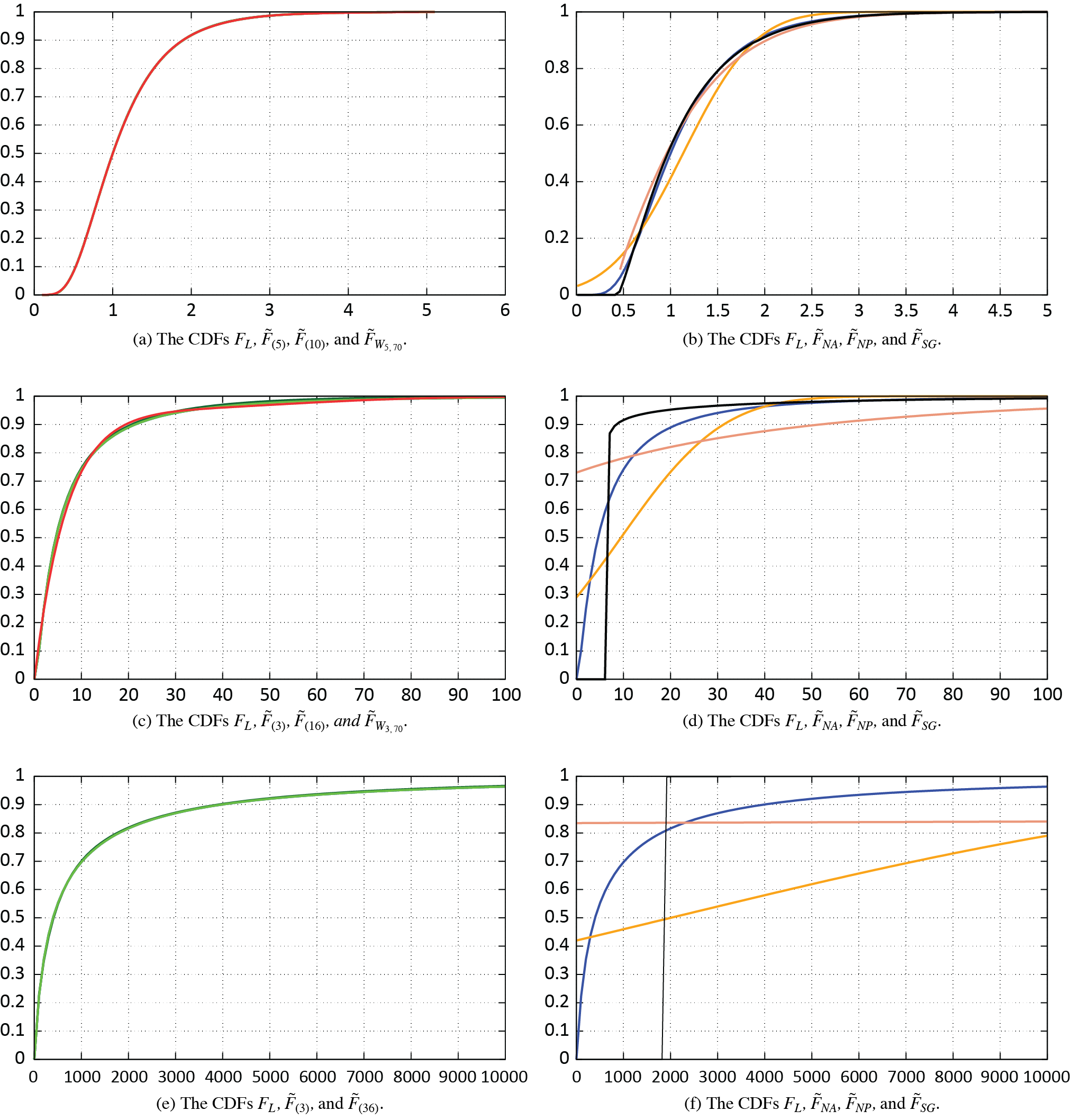
Figure 1 provides the plots of the approximating CDFs in Table 1 as well as the actual CDF F_L (in blue). Figures 1a, 1c, and 1e depict our approximations (dark green and light green, where light green corresponds to the better approximation) and the MED approximation (in red, when applicable). Figures 1b, 1d, and 1f depict the simple moment-matching methods: NA (orange), NPA (salmon), and SGA (black). Apparently, the NA and NPA approximations are inadequate for the more skewed log-normal cases, that is, for the parameterizations (μ = 1.5240, σ = 1.2018) and (μ = 5.9809, σ = 1.8). This is not surprising, as it is well known that the NPA provides fairly accurate results for the skewness values not exceeding one (e.g., Ramsay 1991), whereas the two aforementioned cases of the log-normal distribution lead to the skewness values of 11.23 and 136.38, respectively. In the context of the SGA, higher skewness values imply very small scale parameters, and these in turn result in a nearly vertical rise in the corresponding CDF, thus aggravating the accuracy significantly.

Figure 1.The log-normal CDFs and the corresponding approximations as per Table 1

Example 2. The next distribution we consider is Lomax. As in the case of the log-normal distribution discussed earlier, there is ample of evidence that the Lomax distribution is an adequate model to describing non-life insurance risks. We refer to Seal (1980) for a list of references, and in particular to Benckert and Sternberg (1957), Andersson (1971), and Ammeter (1971) for fire insurance losses, and Benktander (1962) for automobile insurance losses.

Table 2 provides the KS distances for two parameter sets: (α = 2.7163, β = 16.8759), and (α = 2, β = 3000) (e.g., Example 5.7 in Bahnemann 2015). Recall that the mth moment of the Pareto distribution is finite only when m < α. Consequently, most of the existing MMAs are not applicable for these examples; in the first case, only the NA method and MED method with m = 2, are applicable. In contrast, our approximation is feasible in both cases and works well.

Figure 2 compares the plots of the CDFs in Table 2 against the actual CDF F_P (in blue). Figures 2a, and 2c depict our approximations (dark green and light green, where light green corresponds to the better approximation) and the MED approximation (in red, when applicable). Figure 2b depicts the normal approximation (orange).

Figure 2.The Pareto CDFs and the corresponding approximations as per Table 2

Example 3. The final distribution we consider is Weibull, which is a GGC when δ < 1, and these are the values of interest when modeling non-life insurance risks (Bahnemann 2015). Very much like the log-normal and Pareto distributions, the Weibull distribution has been commonly chosen to model insurance data. We refer to Mikosch (2009); Klugman, Panjer, and Willmot (2012) for a general discussion, as well as to Hogg and Klugman (1983) for an application to hurricane loss data.

Table 3 provides the KS distances for the parameters β = 220.653 and δ = 0.8 (e.g., Example 2.13 in Bahnemann 2015).

Figure 3 compares the plots of the CDFs in Table 3 with the actual CDF F_W (in blue). Figure 3a depicts our approximations (dark green and light green, where light green corresponds to the better approximation) and the MED approximation (red). Figure 3b depicts the simple moment-matching methods: NA (orange), NPA (salmon), and SGA (black).

Figure 3.The Weibull CDF and the corresponding approximations as per Table 3

In summary, we note with satisfaction that the proposed refined MMA method has performed exactly as expected in all of the three examples discussed above. That is, it has outperformed all other MMAs in the cases when the latter are applicable (e.g., the lighter-tailed log-normal CDFs with σ = 0.5, σ = 1.2018 and the Weibull CDF), and it has provided a feasible and accurate alternative, otherwise (e.g., the heavier-tailed log-normal CDF with σ = 1.8 and the Pareto CDFs).

We conclude this section by addressing a request of a referee to report the times required to compute the CDFs in Tables 1, 2, and 3 using the MMA approach put forward herein. These times are provided in Table 4. (All calculations were performed on a laptop computer with 12 GB of memory and an IntelCoreTM i5-5200U CPU.) The numbers represent the time, in seconds, required to perform the Gaver Stehfest algorithm described in Section 5 with m = 25 and arithmetic precision to 300 digits and precomputed coefficients of the approximant Laplace transforms. Remarkably, the computation speed can be significantly enhanced (without dramatic drop in accuracy) by reducing the degree of precision and using a smaller value for m. Specifically, we set m = 10 and the arithmetic precision to 100 digits. Then in, e.g., the log-normal case with μ = 5.9809 and σ = 1.8, F̃₍₃₎ and F̃₍₃₆₎ can be computed in 0.948 and 9.396 seconds, respectively, while achieving the KS distances of 7.968e−3 and 1.123e−06, respectively.

We further turn to the aggregate risk RVs, and we demonstrate that the advantages of our approximation method carry on.

6.2. Aggregate risks with full and partial coverage

We begin by approximating the CDF of the RV S_n = X₁ + . . . + X_n - the individual risk model (e.g., Dhaene and Vincke 2004), and the CDF of the RV S_N = X₁ + . . . + X_N - the collective risk model (e.g., Goovaerts 2004). In the former case, we sum n independent RVs with possibly different distributions. In the latter case, we sum a random number N of IID RVs. Furthermore, as ceding insurers often turn to a reinsurer in order to reduce the variability of the underwriting outcomes, we conclude the discussion in this section with the stop-loss reinsurance setup. We note briefly that due to Borch (1969), the variance of the cedent insurer’s payouts is the smallest under the stop-loss reinsurance contract. Irrespective of whether coverage modifications of the aggregate risks are allowed or not, we assume that the stand-alone risks have CDFs (18), (19), and (20). As explicit CDFs of the aggregate risks are not available, we use the Monte-Carlo (MC) method as a benchmark.

Example 4. Consider the CRM, S_N = X₁ + . . . + X_N, where N has a Poisson(λ) distribution, and X_i, i = 1, . . . , N has a log-normal distribution with parameters μ = 5.9809, and σ = 1.8 (Bahnemann 2015, Example 5.9). The Laplace transform of the RV S_N is given by

\[ \phi_{S_{N}}(z)=\exp \left[\lambda\left(\phi_{X_{1}}(z)-1\right)\right] . \]

Thus we obtain an approximation for φ(z) ≔ 𝔼[exp(−zS_N)] as follows

\[ \tilde{\phi}(z)=\exp \left[\lambda\left(\tilde{\phi}_{1}(z)-1\right)\right] . \]

Then we evoke the Gaver-Stehfest algorithm to obtain the approximating CDF of the RV S_N.

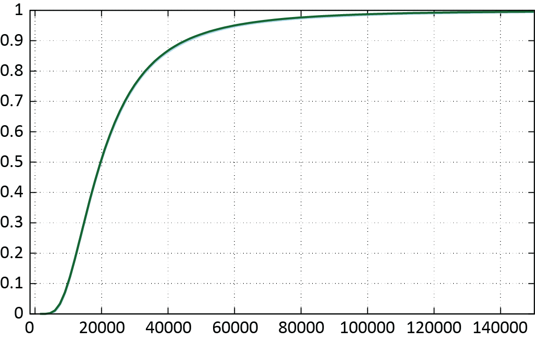
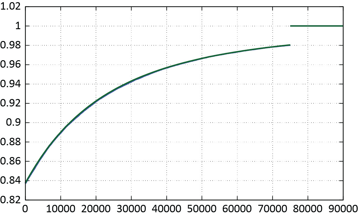
Figure 4 summarizes the results. Namely, Figures 4a, 4c, and 4e show the CDFs of our approximation (dark green; succinctly \(\tilde{F}_{S_N(36)}\) ) and the CDF produced by means of MC simulation with \(10^6\) samples (blue; succinctly \(F_M\) ), for \(\lambda=5,10\), and 15 , respectively. In each one of our approximations, we used \(m=36\) to approximate the underlying log-normal severity distribution. Figures 4b, 4d, and 4f depict the MC CDF (blue), as well as the CDF obtained via NA (orange), NPA (salmon), and SGA (black).

Figure 4.The collective risk model: \(S_N=X_1+\cdots+X_N, N \sim\) Poisson \((\lambda)\), and the \(X_i\) 's are IID log-normally with the parameters ( \(\mu=5.9809, \sigma=1.8\) )

Example 5. Consider the IRM, S_n = X₁ + . . . + X_n, with n = 15. We assume X_i, i = 1, . . . , 5, are distributed log-normally with parameters μ = 5.9809, σ = 1.8, X_i, i = 6,..10, are distributed Pareto with parameters α = 2, β = 3000, and X_i, i = 11, . . . , 15 are distributed Weibull with parameters β = 220.653, δ = 0.8; all independent. The LT of the aggregate risk RV S_n, denoted by φ(z) ≔ 𝔼[exp(−zS_n)], is given by

\[ \phi(z)=\left(\phi_{X_{1}}(z) \cdot \phi_{X_{6}}(z) \cdot \phi_{X_{11}}(z)\right)^{5}. \]

Thus we approximate the CDF of the RV S_n by first approximating the LTs of the severities and then evoking the Gaver-Stehfest method on

\[ \tilde{\phi}(z)=\left(\tilde{\phi}_{1}(z) \cdot \tilde{\phi}_{6}(z) \cdot \tilde{\phi}_{11}(z)\right)^{5} . \]

Figure 5 shows our approximation of the CDF of \(S_n\) (dark green; denoted by \(\tilde{F}_{S_n(40),(36),(30)}\) ) and the CDF obtained by means of MC simulation (blue). In this case, we used approximation orders \(m=40, m=36\), and \(m=30\) to approximate the underlying log-normal, Pareto, and Weibull CDFs, respectively. Note that the RV \(S_n\) has only one finite moment and, hence, other MMAs are not applicable.

Figure 5.The \(\operatorname{CDFs} \tilde{F} S_{n,(40),(36),(30)}\) and \(F M\) for the individual risk model \(S_n\), with \(n=15\)

Example 6. In the previous examples we considered aggregate risks with full coverages, that is there were no deductibles, policy limits, or other policy modifications applied by the insurer to reduce the payouts of the benefits. However, this is not always the case. Consequently, in this example, we explored the so-called stop-loss r.v. S_r,l, which is given, for positive retention r and limit l, by

\[ S_{r, l}=\left\{\begin{array}{ll} 0, & X<r \\ S-r, & r \leq X<r+l \\ l, & r+l \leq X<\infty \end{array}\right. \]

where the RV \(S\) is the aggregate risk RV within either the IRM or CRM. It is a standard exercise to show that the CDF of the RV \(S_{r, l}\) is given by

\[ F_{r, l}(s)=\left\{\begin{array}{ll} \mathbb{P}[S \leq s+r), & s<l \\ 1, & l \leq s \end{array} .\right. \]

Consequently, the CDF of the risk RV \(S_{r, l}\) is approximated similarly to the case in Example 4 (if the RV \(S\) refers to the aggregate risk within CRM), and similarly to the case in Example 5 (if the RV \(S\) refers to the aggregate risk within IRM). To demonstrate, we consider the following CRM: \(S:=S_N=X_1+\cdots+X_N\), \(N \sim\) Poisson(15), and the \(X_i\) 's are IID with log-normal distribution and the parameters \(\mu=5.9809, \sigma=1.8\). For the sake of the demonstration, we set \(r=\mathbb{E}[N] \cdot 3000=45000\), and \(l=\mathbb{E}[N] \cdot 5000=75000\). Figure 6 depicts the approximating \(\operatorname{CDF} \tilde{F}_{r, l}\) of the risk \(\operatorname{RV} S_{r, l}\) (dark green) and the CDF obtained by means of the MC simulation \(F_M\) (blue).

Figure 6.The CDFs \(\tilde{F}_{r, I}\) and FM for the stop-loss contract with retention \(r=45000\) and limit \(I=75000\)

Acknowledgments

We are grateful to the Casualty Actuarial Society (CAS) and the Natural Sciences and Engineering Research Council (NSERC) of Canada for grants supporting our research. Constructive criticism and insightful suggestions of two referees and the editor are also greatly appreciated.