A Comparison of Actuarial Financial Scenario Generators

1. Introduction

In May 2001, the Casualty Actuarial Society (CAS) and the Society of Actuaries (SOA) jointly issued a request for proposals on the research topic “Modeling of Economic Series Coordinated with Interest Rate Scenarios.” The objectives of this request were to develop a research relationship with persons selected to investigate this topic; produce a literature review of work previously done in the area of economic scenario modeling; determine appropriate data sources and methodologies to enhance economic modeling efforts relevant to the actuarial profession; and produce a working model of economic series, coordinated with interest rates, that could be made public via the CAS and SOA websites and used by actuaries to project future economic scenarios. Categories of economic series to be modeled included interest rates, equity price levels, inflation rates, unemployment rates, and real estate price levels. In addition to providing the financial scenario generator model, this project also produced a set of output scenarios for these economic series that could be used directly in financial analysis. This work is summarized in Ahlgrim, D’Arcy, and Gorvett (2004a, 2005).

The Life Capital Adequacy Subcommittee (LCAS) of the American Academy of Actuaries (AAA) recommended in a series of reports (1999, 2002, 2005) that life insurers implement new tests of capital adequacy which utilize stochastic models for scenario testing of variable products with guarantees. Although the ultimate recommendation is for each insurer to develop its own models, the LCAS encouraged the AAA to provide 10,000 prepackaged scenarios that could be used as an alternative to internal models.

As a result of these two projects, practitioners now have a choice between two publicly available financial scenario generators. This paper will serve to explain the underlying processes used in each of the models, compare the output values for common factors, and describe the issues that should be considered when using these models.

The remainder of this paper is organized as follows. Section 2 describes the historical development of actuarial modeling of economic and financial processes, highlighting the growth in popularity of stochastic modeling. Section 3 provides some background on risk-based capital which has become one of the primary uses of stochastic modeling. Section 4 discusses the mathematical and economic details underlying each of the two publicly available financial scenario models. Section 5 analyzes and compares the output and results from each model. Section 6 illustrates the impact of these differences using two separate actuarial applications.

2. Stochastic modeling

Actuarial analysis has progressed through several stages of development regarding the use of economic variables. Initially, the standard approach was to use deterministic values for interest rates, equity returns, and other key financial variables. Judgment was used to estimate the range of expected outcomes and to value embedded options such as investment return and minimum benefit guarantees. This approach often led to the mispricing of key features of insurance policies and consequent financial difficulties for a number of insurers. Many of these problems were due to inadequately reflecting the potential risk and volatility associated with dynamic economic and financial conditions.

Given the disappointing results of deterministic assumptions, actuaries began to recognize the inherent uncertainty surrounding economic variables through predetermined scenarios. For example, New York regulation 126 requires insurers to test asset adequacy and assess their resulting hypothetical financial conditions under seven prescribed interest rate scenarios. Although these prespecified scenarios marked an improvement over the deterministic approach, the use of a limited number of scenarios provided no indication of the relative frequency of any particular outcome, and typically did not reflect the full range of economic conditions that could be expected to occur.

The latest stage in actuarial analysis has been the development of stochastic models to reflect the underlying uncertainty of economic and financial variables (Wilkie 1986, 1995; Hibbert, Mowbray, and Turnbull 2001). When these sophisticated models are properly developed, they can be used to more accurately price embedded options in insurance contracts, to set appropriate solvency margins for diverse insurance operations, and to evaluate alternative operational choices within an insurer. Stochastic models form the basis of dynamic financial analysis (DFA), in which the underwriting and investment components of an insurance company are evaluated, in aggregate, under a large number of potential future environments. Stochastic models are also used in regulation to set risk-based capital (RBC) levels and by rating agencies to establish company ratings.

One of the major concerns raised by the Morris Review of the Actuarial Profession in Great Britain (2004) is that actuaries failed to adequately reflect particular interest rate paths and equity returns over the last decade. Recent advances in the field of financial economics, combined with the increased power and speed of computers, have provided actuaries with powerful stochastic modeling tools. However, understanding the diverse models that have been proposed, and appreciating their underlying philosophical and technical differences, is a significant challenge.

3. Risk-based capital

One of the primary uses of stochastic models is in establishing regulatory capital requirements for insurers. The history of capital standards in insurance shares a similar progression to actuarial assumptions for financial variables. Initial capital standards were simply flat amounts that did not reflect relative risk levels. Minimum margin requirements for European insurers began to be set based on the risks inherent in a company. By the mid-1990s, regulation in the United States, Japan, and other countries moved to an RBC system to define the minimum level of capital an insurer must hold to avoid imposition of regulatory controls. The formula attempted to better correlate an insurer’s inherent risk with its required surplus position. To determine target surplus amounts, RBC factors (or loads) are applied to statutory statement data. Whereas the most dominant risks of life insurers are asset and investment risks, liability and pricing risks are more crucial for property-liability insurers.

3.1. RBC risk types

Since risks have different consequences for each type of insurer, separate RBC formulas have been developed. While the relative weights of risks may be different, the types of risks faced by insurers are identical. Some of these include:

• Asset or investment risks. Capital is required to offset the potential loss in market value of the insurer’s asset portfolio. Higher factors are used for classes of assets that inherently have more risk. For example, the RBC factor applied to stocks is significantly higher than investment grade bonds.

• Insurance/underwriting risks. Given the inevitable random fluctuations in an insurer’s loss experience, RBC is used to protect policy-holders from the inherent uncertainty in an insurer’s liabilities. Since the risk characteristics of each line of business are unique, different capital charges are separately applied to each product. For life insurers, RBC charges are applied to the net amount of risk over and above established reserves. For property-liability lines, the RBC charge is applied to existing loss reserves and written premium amounts.

• Business risks. These charges stem from various risks that may not be covered by other RBC charges, such as loan guarantees to subsidiaries and reinsurance default. While measuring these risks is difficult, the general approach is based on the potential assessment by state guaranty funds.

Life insurers also include a charge for asset-liability management (ALM) risk. In addition to the capital charges levied to reflect the underlying asset risk, an additional layer of risk is present if the values of insurer liabilities are not perfectly coordinated with asset movements. Traditional asset/liability risk is based on the potential mismatch of interest rate sensitivities between the invested assets of the insurer and their policy obligations. For example, if an insurer attempts to obtain a higher interest rate by extending the maturity of their bond portfolio (with no change in the duration of liabilities), the insurer has increased its interest rate exposure. Should yields increase, the value of assets will decline more than the value of the liabilities and the surplus position of the life insurer is impaired. Given the potential for interest rate risk mismatches, the insurer is required to hold a larger amount of capital to support this risk. In the life insurer RBC formula, these risks are termed C-3 risks. In contrast, the value of liabilities for property-liability insurers remains fairly stable with respect to interest rate changes since statutory reserves are not discounted, although the market value of the liabilities would be impacted by interest rate changes (see Ahlgrim, D’Arcy, and Gorvett 2004b and D’Arcy and D’Arcy and Gorvett 2000 for a fuller analysis of this issue).

In the early development of the RBC formula, C-3 risks were coined interest rate risks. Traditional life insurance products are affected by interest rates since the value of policy benefits and policyholder options is closely related to interest rate movements. The potential mismatch between the cash flows of assets and liabilities are most severe with products that have substantial favorable policyholder guarantees (embedded options), notably single premium life products and annuities with rate guarantees. Recent life insurance product development, especially variable annuities and other equity indexed products, pose additional challenges given the heightened sensitivity of liability values to changes in stock market prices. Therefore, the nature of C-3 risks now encompasses broader asset/liability matching risks, not just interest rate risk.

3.2. American Academy of Actuaries RBC guidance

Over time it became evident that the one-size-fits-all application of RBC factors to assess C-3 risk was insufficient to adequately differentiate weakly capitalized insurers from adequately capitalized ones. Given the development of all types of product variations issued by insurers, it was recognized that a single factor which blankets all insurance products would not fit every situation. At the request of the National Association of Insurance Commissioners (NAIC), the Life Risk-Based Capital Task Force of the American Academy of Actuaries began to investigate alternative approaches to better reflect C-3 risk of life insurers.

In October 1999, the task force released its “Phase I Report” (AAA 1999), which provides initial guidance for life insurance companies to measure ALM risks. The report focuses on products with substantial interest rate guarantees, primarily annuities and single premium life products. These guidelines were implemented effective December 31, 2000.

Building upon the modeling techniques that became widespread for asset adequacy testing, the task force recommended scenario testing as a tool for establishing appropriate capital standards instead of the application of RBC factor loadings. The Academy’s aim is to set capital requirements based on the 95th percentile of the distribution stemming from interest rate risks. The Academy’s approach stresses modeling under real-world probability measures. While the risk-neutral measure is important for pricing, it is not useful when estimating the tails of the distribution which ultimately determines the risk exposure for life insurers.

To facilitate development of internal proprietary stochastic models, the Academy provides specific guidance on generating interest rate scenarios. In lieu of developing their own models, companies may choose to use prepackaged scenarios, which are posted on the Academy’s website. Details of their interest rate model are described in Section 4.

The Phase I report acknowledges that C-3 risk consists of more than just interest rate risk. Recent product innovation also incorporates significant equity risk and has greatly expanded the asset/liability risks of insurers. In 2005, the Academy’s task force (now under the name Life Capital Adequacy Subcommittee or LCAS) addressed the equity-related component of C-3 risk by releasing its “Phase II Report” (AAA 2005). These guidelines include “certain standards that must be satisfied” when developing equity return scenarios. For example, Appendix 2 of the June 2005 report includes a “table of calibration points” as a cumulative distribution function of stock returns over various investment horizons.

The LCAS report describes several reasonable approaches to equity modeling. All of these approaches are variations and extensions on the Black-Scholes geometric Brownian motion assumption for stock price movements. While not limiting actuaries to those included, the Academy’s report specifically mentions three equity simulation models:

• Independent lognormal (ILN), where (continuous) stock returns are normally distributed. However, the report highlights the fat-tailed nature of historical stock returns over short horizons that create some difficulty for the ILN approach.

• Two-state regime switching lognormal (RSLN2), where stock returns at any point in time are selected from one of two regimes. The specific regime at each moment is dictated by transition probabilities. It is typical that one regime is characterized by low uncertainty and better stock performance while the other regime has considerable volatility in returns. Extensions of the regime-switching model are possible as well, including varying the time dimension of each period (daily vs. monthly) or incorporating more regimes. The RSLN2 model has received significant publicity by life actuaries. In fact, the original set of scenarios released by the LCAS in 2002 (AAA 2002) was based on the RSLN2 model.

• Stochastic log volatility (SLV), where (log) volatility is a mean-reverting process with constant variance.

4. Model specifications

Two key financial variables of economic models used by insurers are nominal interest rates and equity returns. This section provides details of both the CAS-SOA financial scenario model and the LCAS’s 10,000 scenarios. For reference, the attached Appendix lists and identifies each of the variables included in both scenario generators.

4.1. Interest rates—CAS-SOA model

In the CAS-SOA model, the nominal interest rate is developed from the combined effects of the inflation rate and the real interest rate, each of which is modeled separately.

Inflation (denoted by q) is assumed to follow an Ornstein-Uhlenbeck process of the form (in continuous time):

\[ d q_{t}=\kappa_{q}\left(\mu_{q}-q_{t}\right) d t+\sigma_{q} d B_{q} . \tag{4.1} \]

The simulation model samples the equivalent discrete form of this process:

\[ \begin{aligned} q_{t+1} & =q_{t}+\kappa_{q}\left(\mu_{q}-q_{t}\right) \Delta t+\varepsilon_{q} \sigma_{q} \sqrt{\Delta t} \\ & =\kappa_{q} \Delta t \cdot \mu_{q}+\left(1-\kappa_{q} \Delta t\right) \cdot q_{t}+\varepsilon_{q} \sigma_{q} \sqrt{\Delta t}. \end{aligned} \tag{4.2} \]

From (4.2), we can see that the expected level of future inflation is a weighted average of the most recent value of inflation \(\left(q_t\right)\) and a mean reversion level of inflation, \(\mu_q\). The weight put on the mean reversion level is based on the speed of reversion coefficient parameter \(\kappa_q\). In the continuous model, mean reversion can be seen by considering the first term on the right-hand side of (4.1), called the drift of the process. If the current level of inflation ( \(q_t\) ) is above the average, the drift is negative. In this case, the first equation predicts that the expected change in inflation will be negative-that is, inflation is expected to fall. The second term on the right-hand side represents the uncertainty in the process. In Equation (4.2), this uncertainty is modeled using \(\varepsilon_q\), which is a random draw from a standardized normal distribution. The amount of uncertainty is scaled by the volatility parameter \(\sigma_q\), which is assumed to be constant over time. In the continuous time model (4.1), the random nature of inflation is based on the changes in a Brownian motion \(\left(d B_q\right)\).

The following parameters are used as the “base case” in the model. See Ahlgrim, D’Arcy, and Gorvett (2005) for details about the parameter selection process.

Real interest rates are derived from a simple case of the two-factor Hull-White model (Hull and White 1990). In this model, the short-term rate (denoted by r) reverts to a long-term rate (denoted by l) that is itself stochastic. The stochastic factors are updated over time, analogous to the situation for inflation presented above.

\[ \begin{array}{l} d r_{t}=\kappa_{1}\left(l_{t}-r_{t}\right) d t+\sigma_{1} d B_{1} \\ d l_{t}=\kappa_{2}\left(\mu_{l}-l_{t}\right) d t+\sigma_{2} d B_{2}. \end{array} \]

The discrete analog of the model is:

\[ \begin{aligned} r_{t+1} & =r_{t}+\kappa_{1}\left(l_{t}-r_{t}\right) \Delta t+\sigma_{1} \varepsilon_{1 t} \sqrt{\Delta t} \\ & =\kappa_{1} \Delta t \cdot l_{t}+\left(1-\kappa_{1} \Delta t\right) \cdot r_{t}+\sigma_{1} \varepsilon_{1 t} \sqrt{\Delta t} \\ l_{t+1} & =l_{t}+\kappa_{2}\left(\mu_{l}-l_{t}\right) \Delta t+\sigma_{2} \varepsilon_{2 t} \sqrt{\Delta t} \\ & =\kappa_{2} \Delta t \cdot \mu_{l}+\left(1-\kappa_{2} \Delta t\right) \cdot l_{t}+\sigma_{2} \varepsilon_{2 t} \sqrt{\Delta t} . \end{aligned} \]

In its discrete form, the expected future short rate is a weighted average between the current level r_t and the (stochastic) mean reversion factor l_t. The mean reversion level is itself changing; it is a weighted average of some long-term mean (μ_l) and its current value.

Fisher (1930) provides a thorough presentation of the interaction of real interest rates and inflation and their effects on nominal interest rates. He argues that nominal interest rates compensate investors not only for the time value of money, but also for the erosion of purchasing power that results from inflation. Therefore, when pricing bonds in the CAS/SOA model (i.e., determining the term structure of nominal interest rates), investors’ expectations for inflation and real interest rates over the investment horizon must first be derived.

Using an Ornstein-Uhlenbeck process, Vasicek (1977) provides closed-form solutions for bond prices of all maturities which are simple functions of the underlying process parameters. Therefore, under a stochastic inflationary environment, we denote bond prices at time \(t\) with a maturity of \((T-t)\) as \(P^q(t, T)\). See Hull (2003) for the analogous solutions for the real interest rate process [denoted here as \(P^r(t, T)\)]. Nominal interest rates are then determined by combining the individual effects of inflation and real interest rates over a bond’s maturity:

\[ P^{i}(t, T)=P^{r}(t, T) \times P^{q}(t, T) \]

The following parameters are used in the CAS-SOA model for real interest rates:

4.2. Interest rates—Academy model

While the CAS-SOA model develops nominal interest rates by combining the inflation and real interest rate processes, in the AAA scenarios, nominal interest rates are modeled directly. Appendix 3 of the Phase I report provides some background on the development of the interest rate model used to develop their 10,000 scenarios. According to the report, the goal of their model is to “reproduce as closely as possible certain historical relationships and patterns,” including “minimum and maximum interest rates, the number and length of interest rate inversions, and the absolute and relative distribution of interest rates” (AAA 1999).

Given the inherent focus of RBC on the tail of the distribution, the Academy rejected simple distributional assumptions for interest rates, including normal and lognormal models. As noted in their report, historical interest rate movements had been more “peaked” and “fat-tailed” than those suggested by either distribution, in addition to other shortcomings exhibited by those distributions.

To generate interest rate scenarios, the Academy uses a stochastic (log) volatility model with mean reversion. This interest rate model incorporates changes in three different variables:

• ℓ_t, (the log of) the long-term rate

• φ_t, the spread of long-term rates over short rates

• ν_t, (the log of) the volatility of the long-term rate

Each of these variables in the Academy’s model is assumed to follow a mean reverting process. The Academy’s model has been developed specifically for discrete time simulation; new observations for volatility are generated annually while both the long rate and the spread are sampled monthly. The continuous time equivalent of the model^[1] is:

\[ d\left(\ln \ell_{t}\right)=\kappa_{\ell}\left(\theta_{\ell}-\ln \ell_{t}\right) d t+a \varphi_{t}+\nu_{t} d B_{t}^{\ell} \tag{4.3} \]

\[ d \varphi_{t}=\kappa_{\varphi}\left(\theta_{\varphi}-\varphi_{t}\right) d t+b \ell_{t}+\sigma_{\varphi} d B_{t}^{\varphi} \tag{4.4} \]

\[ d\left(\ln \nu_{t}^{2}\right)=\kappa_{\nu}\left(\theta_{\nu}-\ln \nu_{t}^{2}\right) d t+\sigma_{\nu} d B_{t}^{\nu} . \tag{4.5} \]

\(\theta_{\ell}, \theta_{\varphi}\), and \(\theta_v\) are levels of mean reversion for the long-rate, spread, and volatility, respectively. \(\kappa\) represents the speed of reversion, and \(\sigma\) represents the volatility of the processes. \(a\) and \(b\) are constants. \(B_t^{\ell}\) and \(B_t^{\varphi}\) represent two standard Brownian motions that are correlated with each other, while \(B_t^\nu\) is an independent Brownian motion.

Equation (4.3) shows that the mean reverting process for the long-term rate has stochastic volatility. The volatility of the long rate follows a Gaussian process with constant variance as shown in Equation (4.5). The spread process shown in Equation (4.4) has constant variance. In Equations (4.3) and (4.4), the existing spread influences the movement of the long rate, while the long rate impacts the future spread. These simultaneous equations indicate that the level of interest rates and the spread between long and short interest rates are influenced by the current shape of the term structure.

To create 10,000 scenarios, the AAA sampled long-term interest rates and the yield curve spread [Equations (4.3) and (4.4)] at monthly intervals and sampled the variance of interest rates [Equation (4.5)] at annual intervals based on the following parameters:

In contrast to the CAS-SOA model, closed-form solutions for the entire term structure are not used with the Academy model. Instead, the Academy develops the yield curve from the sampled long- and short-rates from the model. Then, using an iterative procedure, individual interest rates on the term structure are interpolated based on historical relationships among various forward rates [see Appendix III of the Phase I report (AAA 1999) for details].

4.3. Equity returns—CAS-SOA model

The CAS-SOA model uses a regime-switching equity return model, following the approach of Hardy (2001). In this model, at any point in time, stock returns are generated from one of two lognormal distributions called regimes, one with low volatility and one with high volatility. The CAS-SOA model uses the excess equity return which is added to the modeled nominal interest rate for each period to get s_t, the equity return at time t.

\[ \begin{aligned} s_{t} & =r_{t}+q_{t}+x_{t} \\ \ln x_{t} \mid \rho_{t} & \sim N\left(\mu_{\rho_{t}}, \sigma_{\rho_{t}}\right) . \end{aligned} \tag{4.6} \]

Here, \(\rho_t\) represents the regime which dictates the specific distribution of excess returns ( \(x_t\) ) at time \(t\). While more regimes could be incorporated into the model, Hardy’s (2001) work shows that two regimes appear sufficient for both U.S. and Canadian data. Therefore, the CAS-SOA model uses two regimes ( \(\rho_t=1\) or 2). The parameters for large stocks are shown in Table 1. With the regime-switching model, when investors perceive increased uncertainty in the economy, the stock process switches to the high volatility regime. As a result, investors’ increased level of risk aversion leads to falling stock prices (on average). However, given the high uncertainty, stock prices are quite volatile during these times. As investors gather more information and sense normal economic times returning, there is a probability of switching to the low-volatility regime.

4.4. Equity returns—Academy model

The initial guidance by the LCAS (AAA 2002) also used the regime-switching lognormal process for stock returns. However, in the June 2005 report (AAA 2005), the committee released new scenarios based on a stochastic log volatility (SLV) model. The continuous time equivalent of this model is:

\[ d\left[S_{t}\right]=\mu_{t} d t+v_{t} d B_{t}^{s} \tag{4.7} \]

\[ d\left(\ln v_{t}\right)=\phi \times\left[\ln \tau-\ln v_{t}\right] d t+\sigma_{v} d B_{t}^{v} \tag{4.8} \]

\[ \mu_{t}=A+B v_{t}+C v_{t}^{2}. \tag{4.9} \]

The major feature of the SLV model is that (log) volatility follows an Ornstein-Uhlenbeck process with mean reversion level τ and constant volatility σ_v [see Equation (4.8)]. The AAA model constrains the volatility process with upper and lower bounds. Equation (4.9) relates the drift in stock prices to the current level of volatility where A, B, and C are constants. The parameters are chosen where B > 0 and C < 0. The quadratic form of the drift assumption captures two concepts. First, mean-variance efficiency suggests that markets with higher uncertainty receive extra compensation B > 0). Second, given the discrete sampling of the Academy’s scenarios, the quadratic drift captures the effects of volatility on continuously compounded returns. Specifically, the geometric average return over any specific time horizon declines as volatility increases. Thus, C < 0. This risk-return relationship is a bit more com plex than the typical two-stage regime switching model, which often proposes lower returns in the high-volatility regime.

Similar to the interest rate process, the Academy created its scenarios based on monthly sampling of Equations (4.7) through (4.9) and the following parameters (see the Phase II report from AAA 2005 for details):

5. Comparison of results

The approaches used for the CAS-SOA and AAA models both have theoretical support but are quite different from each other. In order to understand these models and when they could be used, it is important to view the values each model generates. Output from the CAS-SOA economic model and the AAA RBC C-3 prepackaged scenarios are compared in several ways. Tables 2–5 list the basic statistics for 10,000 iterations of the CAS-SOA model and the full sample of the 10,000 prepackaged scenarios provided by the AAA RBC C-3 project, along with historical data for the relevant variable. Two types of graphs illustrate the relationship between the two sets of output. One set of graphs displays Redington’s (1952) funnel of doubt graphs over time, showing the 1st, 25th, 50th, 75th, and 99th percentile values for the output distributions from their initial values out through 20 years. This format allows easy comparison of the dispersion reflected in each model. The other type of graph displays a histogram of the model values one year after the start of the simulation, along with historical values of the corresponding variable. These graphs provide a more detailed analysis of the distribution of each variable at a particular point on the funnel of doubt graphs, in this case after one year.

This comparison indicates significant differences between the two models, especially for interest rates. Based on Table 2, the mean value of the 3-month nominal interest rate for the CAS-SOA model after one year, at 3.28%, demonstrates faster reversion to the long-run mean than is reflected in the AAA RBC C-3 scenarios, at 2.97%. The standard deviation of the CAS-SOA model of 2.7% is much higher than the standard deviation of the AAA RBC C-3 scenarios, at 1.4%, and the skewness of the CAS-SOA model is .620, compared to .249 for the AAA model. Based on each value, the CAS-SOA model produced results closer to the historical (1934–2006) values. The only statistic for which the CAS-SOA model did not produce closer agreement was for kurtosis, which in both models is negative (−.230 and −.189), compared to the historical value of .970.

Figure 1 illustrates the differences in levels and dispersion for the 3-month nominal interest rate of the two models over a 20-year horizon. Both models start at approximately the same level (CAS-SOA at 1.0% and the AAA at 1.21%), but the CAS-SOA model increases faster and to a higher level with greater dispersion.^[2] Even after 20 years, the AAA scenarios indicate a less than 1% chance of 3-month interest rates exceeding 13%, even though this value has been as high as 16% within the last 30 years. The histogram displayed in Figure 2 shows the distribution of 3-month nominal interest rates after one year. The values for the AAA scenarios are almost entirely within the range of 1% to 5%. The CAS-SOA model has a much wider distribution, although not as wide as the historical values.

Figure 1.Funnel of doubt graphs: 3-month nominal interest rates

Figure 2.Three-month nominal interest rates: model values and actual data (01/34–01/06)

Comparing the results for the 10-year nominal interest rates produces a similar pattern. From Table 3, the CAS-SOA values have a higher mean, 5.1% to 4.6%, and standard deviation, 1.3% to 0.7%, than the AAA scenarios. Actual values are only available for this data series from 1953–2006, with a mean of 6.5%. Neither model generates values for kurtosis or skewness that are close to the limited period of historical values that are available, but the signs of the AAA scenarios are both positive, in line with actual values. The funnel of doubt graphs in Figure 3 are both higher and wider for the CAS-SOA values than the AAA scenarios, except after 15 years. After this point, the AAA scenarios produce a 99th percentile value above the values the CAS-SOA model produces, but the 50th and 75th percentile values are still lower. Figure 4 shows the distribution of the CAS-SOA model is wider than the AAA scenarios. Both are much lower than the historical values shown in the figure. However, this discrepancy might not be a problem. Current interest rates, which are low by historical standards, are used as the starting point for both interest rate models. Despite mean reversion, high interest rates are less likely to occur within a year than they would be if interest rates were starting at a higher level. However, from July 1980 to July 1981, 10-year interest rates increased by 403 basis points, so the limited range of the AAA model might be considered too restricted.

Figure 3.Funnel of doubt graphs: 10-year nominal interest rates

Figure 4.Ten-year nominal interest rates: model values and actual data (04/53–01/06)

Table 4 provides the basic statistics for large stock total returns for both models and for historical values, based on the S&P 500 and its predecessor, the Cowles Index. The mean of the CAS-SOA model is 8.7%, and the mean for the AAA scenarios is 9.0%, both close to the historical value of 10.4%. The standard deviation of the CAS-SOA model, at 22.1%, is higher than the AAA scenarios, at 16.6%, and the historical values, at 17.8%. The effect of the larger standard deviation is evident in the 99th and 1st percentile values (largest 100 and smallest 100). These values are 62.7% and −52.6% for the CAS-SOA model, but only 51.7% and −30.0% for the AAA scenarios. The AAA scenarios are in line with the largest and smallest returns of the S&P 500 (53.8% and −31.2%, respectively) over the 135-year period.

The funnel of doubt graphs of Figure 5 narrow over time, rather than expand, due to the way stock returns are generated in the two models. Stock return values represent the cumulative average annual returns from investing in large stocks over the indicated time period. This produces a portfolio effect over time, as large gains or losses in one year are likely to be moderated by the returns of the remaining years in the investment horizon. Thus, the funnel of doubt is inverted, with returns more predictable for a 20-year investment horizon than for a single year. Since the standard deviation of returns is smaller under the AAA approach, the compounded average returns over longer periods converge more quickly. This difference is the result of the different approaches to the model, with the CAS-SOA model using regime switching and the AAA model based on the stochastic log volatility model. The histogram in Figure 6 for large stock returns after one year (which are measured similarly for both models) illustrate the similar dispersion for the two models, both in line with actual values.

Figure 5.Funnel of doubt graphs: large stock return (US equity)

Figure 6.Large stock return: model values and actual data (1872–2006)

The results for small stock returns are indicated in Table 5. In this case the CAS-SOA results are closer to historical values. The mean value of the CAS-SOA model is 13.6%, compared with a mean of the AAA model of 10.3% and the historical mean of 17.5%. The standard deviation of the CAS-SOA model, at 35.1%, is closer than the AAA scenarios, at 22.6%, to the historical value of 33.1%. The 99th and 1st percentile values are 129.7% and −61.8% for the CAS-SOA and 70.7% and −39.6% for the AAA. In this case the CAS-SOA results are closer to the historical range of 142.9% and −58.0% over a 79-year period. The greater initial dispersion of the CAS-SOA model is evident in Figure 7. The histogram on Figure 8 provides another illustration of the greater dispersion of the CAS-SOA model.

Figure 7.Funnel of doubt graphs: small stock return (intermediate risk equity)

Figure 8.Small stock returns: model values and actual data (1926–2004)

Although the goal of each model is to provide a reasonable distribution of potential future financial values, which cannot be quantified ex ante, it is possible to compare the output from the models to historical data to measure how well the models fit past experience. Two quantitative metrics are used to test how closely the output from the models conforms to historical values. The Kolmogorov-Smirnov (K-S) test measures whether two datasets, in this case output from each model and actual observations, are significantly different. This test does not depend on knowing the distribution of the underlying data, and therefore is not as sensitive as tests based on specific distributions. The second test is the chi-square test that compares the distribution of output from the model to the distribution of actual observations.

It should be noted that the models were not developed solely to replicate history. Instead, the models are intended to provide a reasonable framework for understanding potential future uncertainty. Often, when choosing parameters for economic and financial models, users exploit historical relationships in time series data. Any test statistic that measures historical fit is influenced by the weight given to past data. When parameters are selected entirely from historical movements, statistical fit is likely to be affected. In particular, historical fit is likely to look better if there is significant overlap between the time period used for parameter estimation and the time period used to measure historical fit. Readers should keep this in mind when looking at measures of fit across competing models.

The K-S test is illustrated graphically for 3-month nominal interest rates in Figure 9. The cumulative distributions for historical interest rates and both models (CAS-SOA and AAA) are shown. The K-S test metric D is the maximum vertical difference between the cumulative distribution of the actual data and cumulative distribution of each model. By comparing the D values for the two models, we can determine which model produces the better fit. Based on Figure 9, the CAS-SOA model has a lower D and thus provides a better fit to historical observations for 3-month interest rates. In running this test, 10 subsets of 1,000 observations each were drawn from the two models and the D values calculated for each subset. The results are displayed in Table 6. For each variable, 3-month and 10-year interest rates and large and small stocks, the CAS-SOA model generated lower D values and therefore produced a better fit.

Figure 9.Three-month nominal interest rates: K-S test results

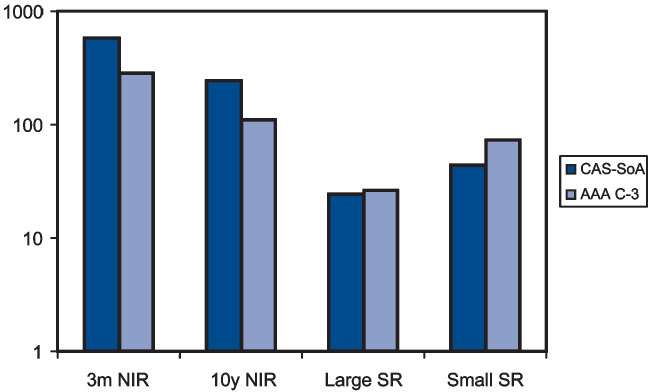
Secondly, the chi-square method is used to test the difference between the model output and actual values. The chi-square measure is the squared difference between observed frequency (O) and the expected frequency (E), which is then divided by the expected frequency. In this case, observed frequency is the distribution of historical interest rates or equity returns. Expected frequency is the distribution of model values from the underlying “known” distributions as generated from CAS-SOA or AAA-C-3 models. The sum of the differences between these values from each of the multiple frequency intervals is the chi-square statistic, as shown in Equation (5.1).

\[ \chi^{2}=\sum \frac{(O-E)^{2}}{E} . \tag{5.1} \]

There are 42 bins based on 50 basis point intervals for interest rates and 17 bins (for large stocks) or 29 bins (for small stocks) based on 500 basis point intervals for equity returns. The results of chi-square test on both models are shown in Figure 10. For all cases the null hypothesis (that the model and observations are drawn from the same distribution) is rejected at the 10% level. However, the models do generate slightly different values for this metric. In general, the AAA model produces interest rates that correspond more closely to historical distributions, whereas the CAS-SOA model generates equity returns that correspond more closely with historical values. The objective of the models, though, is to project the potential distribution of future interest rates and equity returns, not to replicate distributions of historical values.

Figure 10.Chi-square test

6. Cash flow testing

In order to illustrate the differences between the CAS-SOA financial scenario model and the AAA C-3 model, two simple examples are demonstrated here. The first example is a $100,000 face value, single premium, 10-year term life insurance policy for a 35-year-old male. The net premium of $2,423 is determined by discounting the death benefits assuming 1980 CSO mortality rates and an interest rate of 3.5%. The single premium is invested in a portfolio that is allocated 50% to 3-month Treasury bills, 25% to large stocks, and 25% to small stocks. The investment performance of each category is based on 10,000 iterations of the competing financial models. At the end of each year, death benefits are paid based on the assumed mortality table. In this simplified example, only the investment performance is assumed to be stochastic; a more realistic example would incorporate stochastic mortality rates, company expenses, and policy cancellations. However, these situations are beyond the scope of this project.

The results of this exercise are shown as funnel of doubt graphs in Figure 11, and numerically in Tables 7A and 7B. The CAS-SOA model generates a higher mean value at the end of each year, a much wider range and a greater chance of the net premium proving inadequate in every year except year 10. At the end of 10 years, the mean value of the insurer’s surplus is $1,700 based on the CAS-SOA model and $574 based on the AAA C-3 model. This positive surplus is not surprising given that, on average, the insurer is expected to earn more than the assumed 3.5% used in the calculation of premiums. In addition, since the CAS-SOA model projects higher interest rates and higher returns on small stocks, the insurer’s surplus position would increase, on average. However, in 22.0% of the iterations for the CAS-SOA model and 26.9% of the iterations for the AAA C-3 model, the projected surplus of the life insurer was negative, indicating a loss was incurred on the policy. The higher expected returns notwithstanding, the greater volatility represented by the CAS-SOA model produces a large portion of cases where the premium is inadequate for the coverage provided.

Figure 11.Funnel of doubt graphs for life insurance example

The second example is based on a property-liability loss reserve situation. In this case, a loss reserve of $10 million is established, which is supported by $10 million in assets, because property-liability insurance accounting does not permit discounting of loss reserves. The assets are invested in the same portfolio used for the life insurance example (50% 3-month Treasury bills, 25% large stocks, and 25% small stocks). The loss payments are $1 million per year, paid at the end of each year for 10 years. (More realistic loss payout patterns could be substituted for this uniform set of payments, but the purpose of this example is only to indicate an approach to compare the two models, and is not dependent on a specific payout pattern. As in the prior example, stochastic loss payouts should be incorporated in actual cash flow tests.) The funnel of doubt graphs in Figure 12 and the numerical values in Tables 8A and 8B show the residual value of the portfolio each year. In both cases, the investment returns, on average, are large enough to pay all the losses over the 10 years, with a mean residual value of $10.4 million for the CAS-SOA model and $5.5 million for the AAA C-3 model. The dispersion of the residual value at the end of 10 years is much greater for the CAS-SOA model, with a standard deviation of $9.9 million, compared to $3.7 million for the AAA C-3 model. In 6.3% of the iterations for the CAS-SOA model and in 2.8% of the iterations for the AAA C-3 model, the residual values at the end of 10 years were negative. In these cases, even undiscounted loss reserves would be inadequate to cover the liabilities.

Figure 12.Funnel of doubt graphs for property-liability loss reserve example

The striking differences in results illustrated above clearly demonstrate the importance of selecting an appropriate model for use in cash flow testing. Solvency margins, pricing strategies, capital allocations, and investment strategies all depend on using valid models for economic conditions. That two models, both developed around the same time for similar purposes and using comparable approaches for modeling interest rates and equity movements, can produce such widely divergent results emphasizes the care that must be taken in developing, parameterizing, and applying financial models to insurance operations. Just using a stochastic model is not sufficient. The model must be a valid one, with parameters that reflect current economic conditions, and the model must be applied appropriately.

7. Conclusions

Both the CAS-SOA model and the AAA prepackaged scenarios provide values for interest rates and equity returns that can be used in actuarial modeling. The different approaches used in each procedure lead to significant differences in the resulting output. The CAS-SOA model leads to a wider set of distributions, especially for interest rates, than the AAA scenarios. Before adopting either approach, the user should understand the factors considered by each model and how their specific application may be affected by the output.