1. Introduction
Over the years, there has been an increasing recognition that consideration of the random nature of the insurance loss process leads to better predictions of ultimate losses. Some of the papers that led to this recognition include Stanard (1985) and Barnett and Zehnwirth (2000). Another thread in the loss reserve literature has been to recognize outside information in the formulas that predict ultimate losses. Bornhuetter and Ferguson (1972) represents one of the early papers exemplifying this approach.
More recently, papers by Meyers (2007) and Verrall (2007) have combined these two approaches with a Bayesian methodology. This paper continues the development of the approach started by Meyers and draws from the methodology described by Verrall.
A significant accomplishment of the Meyers paper cited above was that it made predictions of the distribution of future losses of real insurers, and successfully validated these predictions on subsequent reported losses. To do this, it was necessary to draw upon proprietary data that, while generally available, comes at a price. While this made a good case that the underlying model is realistic, it tended to inhibit future research on this methodology. This paper uses nonproprietary data so that readers can verify all calculations. In addition, this paper includes the code that produced all results and, with minor modifications, it should be possible to use this code for other loss reserving applications.
2. The collective risk model
This paper analyzes a 10 × 10 triangle of incremental paid losses organized by rows for accident years 1, 2, . . . ,10 and by columns for development lags 1, 2, . . . ,10. We also have the premium associated with each accident year. Table 1 gives the triangle that underlies the examples in this paper.
Table 1.Incremental paid losses (000)
| 1 |
50,000 |
7,168 |
11,190 |
12,432 |
7,856 |
3,502 |
1,286 |
334 |
216 |
190 |
0 |
| 2 |
50,000 |
4,770 |
8,726 |
9,150 |
5,728 |
2,459 |
2,864 |
715 |
219 |
0 |
|
| 3 |
50,000 |
5,821 |
9,467 |
7,741 |
3,736 |
1,402 |
972 |
720 |
50 |
|
|
| 4 |
50,000 |
5,228 |
7,050 |
6,577 |
2,890 |
1,600 |
2,156 |
592 |
|
|
|
| 5 |
50,000 |
4,185 |
6,573 |
5,196 |
2,869 |
3,609 |
1,283 |
|
|
|
|
| 6 |
50,000 |
4,930 |
8,034 |
5,315 |
5,549 |
1,891 |
|
|
|
|
|
| 7 |
50,000 |
4,936 |
7,357 |
5,817 |
5,278 |
|
|
|
|
|
|
| 8 |
50,000 |
4,762 |
8,383 |
6,568 |
|
|
|
|
|
|
|
| 9 |
50,000 |
5,025 |
8,898 |
|
|
|
|
|
|
|
|
| 10 |
50,000 |
4,824 |
|
|
|
|
|
|
|
|
|
Let XAY, Lag be a random variable for the loss in the cell (AY, Lag). Our job is to predict the distribution of the sum of the losses, ΣXAY, Lag in the empty cells (AY+Lag>11).
Let us start by considering two models for the expected loss.
Model 1—The Independent Factor Model
E[LossAY, Lag ]=PremiumAY⋅ELRAY⋅DevLag.
The unknown parameters in this model are ELRAY(AY=1,2,…,10), representing the expected loss ratio for accident year AY, and DevLag(Lag=1,2,…,10 ), representing the incremental paid loss development factor. The DevLag parameters are constrained to sum to one. The structure of the parameters is similar to the “Cape Cod” model discussed in Stanard (1985) but, as we shall see, this paper allows the ELRAY parameters to vary by accident year.
Model 2—The Beta Model
In the Independent Factor model, set
DevLag=β( Lag /10∣a,b)−β(( Lag −1)/10∣a,b)
where β(x | a,b) is the cumulative probability of a beta distribution with unknown parameters a and b as parameterized in Appendix A of Klugman, Panjer, and Willmot (2004).
The Beta model replaces the 10 unknown DevLag parameters in the Independent Factor model with the two unknown parameters a and b. I chose these models as representatives of a multitude of possible models that can be used in this approach. Other examples in this multitude include the models in Meyers (2007), who uses a model with constraints on the DevLag parameters, and Clark (2003), who uses the Loglogistic and Weibull distributions to project DevLag parameters into the future.
We describe the distribution of XAY, Lag by the collective risk model, which can be described by the following simulation algorithm:
Simulation Algorithm 1
- Select a random claim count, NAY,Lag from a Poisson distribution with mean λAY,Lag.
- For i=1,2,…,NAY, Lag , select a random claim amount, ZLag,i.
- Set XAY, Lag =∑NAY Lag i=1ZLag,i, or if NAY, Lag =0, then XAY,Lag=0.
Using the collective risk model assumes that one has a claim severity distribution. Meyers (2007) uses claim severity distributions from his company. In keeping with the “disclose all” intent of this paper, we use the Pareto distribution, as an example, with the cumulative distribution function:
F(z)=1−(θfz+θf)αf.
We set αf=2 and let θf vary by settlement lag as noted in Table 2. All claims are subject to a limit of $1 million.
Table 2.pθf for claim severity distributions
| θf(000) |
10 |
25 |
50 |
75 |
100 |
125 |
150 |
Note that the average severity increases with the settlement lag, which is consistent with the common observation that larger claims tend to take longer to settle.
To summarize, we have two models (the independent factor and the beta) that give E[XAY, Lag ] in terms of the unknown parameters {ELRAY} and {DevLag}. We also assume that the claim severity distributions of ZLag are known. Then for any selected {ELRAY} and {DevLag}, we can describe the distribution of XAY,Lag by the following steps.
-
Calculate
λAY, Lag =E[XAY, Lag ]E[ZLag]= Premium AY⋅ELRAY⋅ Dev LagE[ZLag].
-
Generate the distribution of XAY, Lag using Simulation Algorithm 1 above.
3. The likelihood function
Let X denote the data in Table 1. Let ℓ(X∣{ELRAY},{DevLag}) be the likelihood (or probability) of X given the parameters {ELRAY} and {DevLag}. Note that defining a distribution in terms of a simulation algorithm does not lend itself to calculating the likelihood. There are two ways to overcome this obstacle. Meyers (2007) calculates the likelihood of X by finely discretizing the claim severity distributions and using the Fast Fourier Transform (FFT) to calculate the entire aggregate loss distribution—a time-consuming procedure if one needs to calculate a single probability repeatedly, as this paper does.
Instead of using the FFT to calculate the likelihood, this paper approximates the likelihood by using the Tweedie distribution in place of the collective risk model described in Simulation Algorithm 1. Smyth and Jørgensen (2002) describe the Tweedie distribution as a collective risk model with a Poisson claim count distribution and a gamma claim severity distribution.
Let λ be the mean of the Poisson distribution. Let θt and αt be the scale and shape parameters of the gamma claim severity distribution, f(x)=(x/θt)αte−x/θt/x⋅Γ(αt). The expected claim severity is given by τ=αt⋅θt. The variance of the claim severity is αt⋅θ2t. Smyth and Jørgensen (2002) parameterize the Tweedie distribution with the parameters p,μ and ϕ, with
p=αt+2αt+1,μ=λ⋅τ, and ϕ=λ1−p⋅τ2−p2−p=μ1−p⋅τ2−p.
With this parameterization, the mean of the Tweedie distribution is equal to μ, and the variance is equal to ϕ⋅μp. The Tweedie distribution does not have a closed form expression of its density function.
The approximation is done by selecting a gamma distribution within the Tweedie that has the same first two moments of the Pareto distributions specified above. For a given (AY, Lag) cell, let t(XAY, Lag ∣ELRAY,DevLag) denote the density of the approximating Tweedie distribution. Appendix B gives a detailed description of how the density of the Tweedie distribution is calculated in this paper. For the entire triangle, X, the likelihood function is given by
ℓ(X∣{ELR},{Dev})=10∏AY=111−AY∏Lag=1t(xAY,Lag∣ELRAY, Dev Lag).
The Tweedie approximation leads to much faster running times for the algorithms described in this paper. Other papers using the Tweedie distribution in loss reserve analysis include Taylor (2009), Peters, Shevchenko, and Wüthrich (2009), and Wüthrich (2003).
The maximum likelihood estimator has been historically important. Many prefer it because it does not depend on prior information. Over the past decade or so, a number of popular software packages began to include flexible function-maximizing tools that will search over a space that includes a fairly large number of parameters. Excel Solver is one such tool. With such a tool, the software programs that accompany this paper calculate the maximum likelihood estimates for the Independent Factor and the Beta models.
The Independent Factor program calculates the maximum likelihood estimate by searching over the space of {ELRAY} and {DevLag}, subject to a constraint that ∑10Lag=1DevLag=1. The Beta program feeds the results of Equation 2 into the likelihood function used in the Independent Factor program as it searches over the space of {ELRAY},a and b. Table 3 gives the maximum likelihood estimates for each model.
Table 3.Maximum likelihood estimates
| ELR |
Dev |
ELR |
Dev |
| 1 |
0.88832 |
0.16760 |
0.88496 |
0.16995 |
| 2 |
0.67147 |
0.27635 |
0.65567 |
0.26388 |
| 3 |
0.64720 |
0.23451 |
0.65236 |
0.23094 |
| 4 |
0.56222 |
0.15660 |
0.55986 |
0.16322 |
| 5 |
0.49539 |
0.07751 |
0.48969 |
0.09764 |
| 6 |
0.57450 |
0.04825 |
0.57342 |
0.04885 |
| 7 |
0.58392 |
0.02267 |
0.57112 |
0.01936 |
| 8 |
0.56703 |
0.01101 |
0.59260 |
0.00536 |
| 9 |
0.60360 |
0.00108 |
0.63075 |
0.00077 |
| 10 |
0.54760 |
0.00443 |
0.56753 |
0.00002 |
|
|
|
|
a = 1.75975 |
|
|
|
|
b = 5.25776 |
4. The prior distribution of model parameters
Let us now develop the framework for a Bayesian analysis. The likelihood function ℓ(X∣{ELRAY},{DevLag}) is the probability of X, given the parameters {ELRAY} and {DevLag}. Using Bayes’ Theorem, one can calculate the probability of the parameters {ELRAY} and {DevLag} given the data, X.
Pr{{ELRAY},{DevLag}∣X}∝ℓ(X∣{ELRAY},{DevLag})⋅Pr{{ELRAY},{DevLag}}.
A discussion of selecting the prior distribution Pr{{ELRAY},{DevLag}} is in order. This paper uses illustrative data so it is editorially possible to select anything as a prior distribution. However, I would like to spend some time to illustrate one way to approach the problem of selecting the prior distribution when working with real data.
Actuaries always stress the importance of judgment in setting reserves. Actuarial consultants will stress the experience that they have gained by examining the losses of other insurers. Meyers (2007) provides one example of a way to select a prior by examining the maximum likelihood estimates of the {DevLag} parameters from the data of 40 large insurers. In an effort to keep the examples in this paper as realistic as possible, I looked at the same data and selected the prior distribution as follows.
Beta Model:
a∼Γ(αa,θa) with αa=75 and θa=0.02
b∼Γ(αb,θb) with αb=25 and θb=0.20.
Figure 1 shows the DevLag paths generated from a sample of fifty (a,b) pairs sampled from the prior distribution.
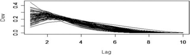
Figure 1.Development paths
For the Independent Factor model, I calculated the mean and variance of the DevLag parameters simulated from a large sample of (a,b) pairs and selected the following parameters in Table 4 for the gamma distribution for each DevLag.
Table 4.Prior distribution of settlement lag parameters
| αd |
11.0665 |
64.4748 |
189.6259 |
34.8246 |
10.6976 |
4.4824 |
2.1236 |
1.0269 |
0.4560 |
0.1551 |
| θd |
0.0206 |
0.0041 |
0.0011 |
0.0040 |
0.0079 |
0.0101 |
0.0097 |
0.0073 |
0.0039 |
0.0009 |
I also use the gamma distribution as the prior for {ELRAY}. By similarly looking at the Meyers (2007) data, I selected the parameters αe=100 and θe=0.007 for the prior gamma distribution.
5. The Metropolis-Hastings algorithm
In a Bayesian analysis, computing the posterior distribution can be difficult. Given a conditional distribution with probability density, f(x | μ), and a prior distribution, g(μ), the posterior distribution is given by f(x) = ʃ0∞ f(x | μ)· g(μ)dμ. If, for example, f(x | μ) is given by a Tweedie distribution and g(μ) is given by a gamma distribution, the integral does not have a closed-form solution. While numerically evaluating this integral may be feasible if μ has only one or two dimensions, it is practically impossible when μ has many dimensions. The Beta model and the Independent Factor models have 12 and 19 parameters, respectively.
A recent trend in Bayesian statistics has been to use Markov Chain Monte-Carlo (MCMC) methods to produce a sample {μi} to describe the posterior distribution of μ. This section describes one of the more prominent MCMC methods called the Metropolis-Hastings algorithm. Three references on MCMC methods that I have found to be useful are Albert (2007), Wüthrich and Mertz (2008), and Lynch (2007).
First, let’s describe the idea behind MCMC methods. A Markov chain is a sequence of random variables that randomly moves from state to state over discrete units of time, t. The probability of moving to a given state at time t depends only on its state at time t − 1. The term “Monte-Carlo” refers to a computer-driven algorithm that generates the Markov chain.
The Metropolis-Hastings algorithm starts with a proposal density function, p, and an initial value, μ1. It then generates successive μt s according to the following simulation algorithm.
Simulation Algorithm 2
- Select a random candidate value, μ∗ from a proposal density function p(μ∗∣μt−1).
- Compute the ratio
R=f(x∣μ∗)⋅g(μ∗)⋅p(μt−1∣μ∗)f(x∣μt−1)⋅g(μt−1)⋅p(μ∗∣μt−1).
- Select a random number U from a uniform distribution on (0,1).
- If U<R then set μt=μ∗. Otherwise set μt= μt−1.
An example of a proposal density function is p(μ∗∣μt−1)=Φ(μ∗∣μt−1,σ), where here, Φ() is the density function for a normal distribution with mean μt−1 and standard deviation σ. Note that if we choose this proposal density function, p(μ∗∣μt−1)=p(μt−1∣μ∗) and the p s cancel out when calculating the ratio R. Another choice for a proposal density function would be p(μ∗∣μt−1) =Γ(μ∗∣μt−1/αp,αp), a gamma distribution with shape parameter αp, and scale parameter μt−1/αp. The mean of this gamma distribution is μt−1. A gamma proposal density function will assure that μt is not negative.If the selection of the μ∗ leads to a high value of the ratio, R,μt=μ∗. If the selection of μ∗ leads to a low value of R, depending on the randomly selected value of U,μt can be either μ∗ or μt−1. Thus μt will tend to move around the high density regions of the posterior distribution of μ, yet occasionally venture into the low-density regions of the posterior distribution. It has been demonstrated mathematically that as t approaches infinity, the distribution of the μt s converges to the posterior distribution of μ. See Lynch (2007) for further references on this.
The convergence rate is controlled by the variability of the proposal density function. For the normal proposal density function above, a low value of σ will have the result that μt moves slowly and convergence will be slow. A high value of σ will lead to a more frequent rejection of μ∗ in Step 4 of the algorithm, and hence slow convergence of the μt s with the frequent occurrence of μt=μt−1. Similarly, the choice of αp influences the convergence rate for the gamma proposal density function. The practice that seems to be evolving among practicing Bayesians is one of choosing a proposal density volatility parameter, by trial and error, that results in about a 50% acceptance rate in Step 4 for single parameter posterior distributions, and about a 25% acceptance rate for multi-parameter posterior distributions.
Let’s look at an example. Table 5 shows 25 observed losses, denoted by Y.
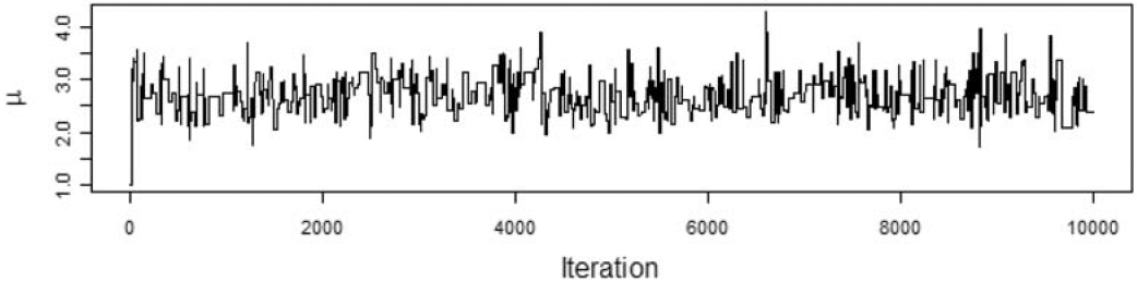
We want to model the losses with a Tweedie distribution with parameters ϕ=1,p=1.5, and unknown mean, μ. The prior distribution of μ is a gamma distribution with αμ=5 and θμ=1. To illustrate the effect of the choice of the proposal distribution, I ran the Metropolis-Hastings algorithm using the gamma proposal distributions with αp=2500,αp=25, and αp=0.25. The acceptance rate for the each run was 95%, 56%, and 6%, respectively. Figures 2, 3, and 4 show the paths taken by the values of μ for 10,000 iterations for each value of αp. Bayesian statisticians call these “trace plots.”
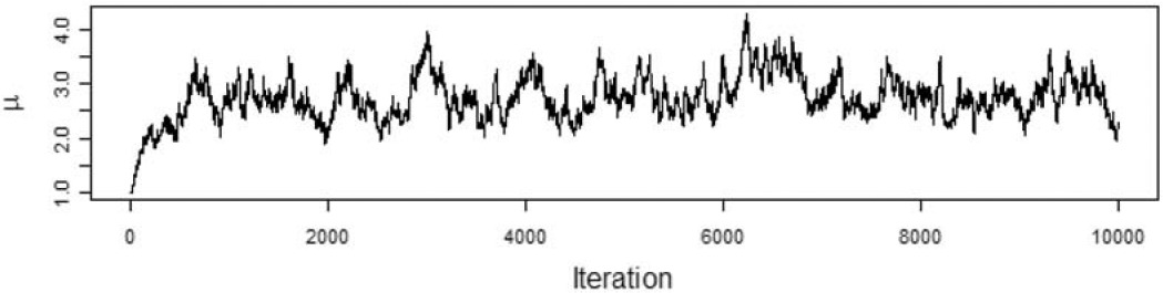
Figure 2.αp=2,500
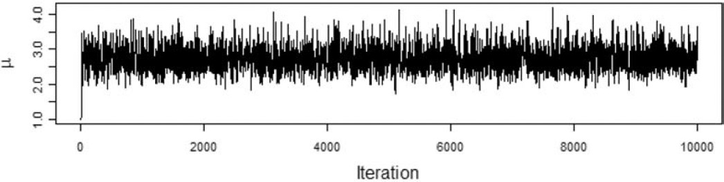
Figure 3.αp=25

Figure 4.αp=0.25
Figure 2 shows a high degree of autocorrelation between successive iterations because of the low volatility (i.e., small steps) taken by the proposal density function. Figure 4 shows a high degree of autocorrelation because of the frequent rejection of μ* taken because of the high volatility of the proposal density function.
Because of the irregular cycles in Figures 2 and 4 caused by autocorrelation, one needs to run a large number of iterations to get a good approximation to the posterior distribution. It took a smaller number of “burning” iterations to reach the steady state in Figure 3.
Figure 5 gives a histogram representing the posterior distribution of μ by a histogram consisting of the μts generated by the last 5,000 iterations of the Metropolis-Hastings algorithm. This might be referred to as the distribution of “reasonable estimates.”
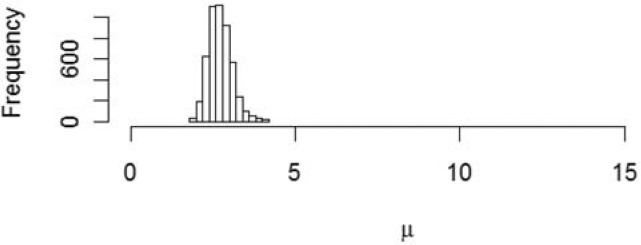
Figure 5.Posterior distribution of μ
In addition to the distribution of estimates, one often wants the predictive distribution of outcomes, Y. As the algorithm produced each μt, I also programmed it to take a random Y from a Tweedie distribution with parameters ϕ=1,p= 1.5, and μt. Figure 6 gives a histogram of this predictive distribution.
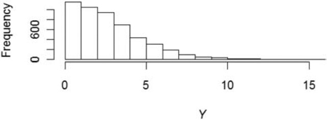
Figure 6.Predictive distribution of Y
6. The posterior distribution of model parameters
This section illustrates one way of using the Metropolis-Hasting algorithm to generate the posterior distribution of the model parameters. The Metropolis-Hastings algorithm for these models is implemented in two steps. The first step selects the {DevLag} parameters and the second step selects the {ELRAY} parameters.
For Beta model I used the maximum likelihood estimates of the a,b, and {ELRAY} parameters as the starting values a1,b1, and {ELRAY}1. For the proposal density function, I used a gamma distribution, p(x∗∣xt−1)=Γ(x∗∣xt−1/α,α) with shape parameter α=500 for x=(a,b) and {ELRAY} as needed. Successive at,bt, and {ELRAY}t parameters were generated by the following simulation algorithm. As appropriate, g will denote the prior distributions of the parameters a,b, and {ELRAY}.
Simulation Algorithm 3
-
Select random candidate values, a∗ and b∗, from the proposal density function p((a∗,b∗)∣ (at−1,bt−1)).
-
Compute the ratio:
R=ℓ(X∣{ELRAY}t−1,{DevLag∣a∗,b∗})g(a∗,b∗)⋅p(at−1,bt−1∣a∗,b∗)ℓ(X∣{ELRAY}t−1,{DevLag∣at−1,bt−1}).
-
Select a random number U from a uniform distribution on (0, 1).
-
If U<R then set (at,bt)=(a∗,b∗). Otherwise set (at,bt)=(at−1,bt−1).
-
Select random candidate values {ELRAY}∗ from the proposal density function p({ELRAY}∗ ∣{ELRAY}t−1).
-
Compute the ratio:
R=ℓ(X∣{ELRAY}∗,{DevLag∣at,bt})g({ELRAY}∗)⋅p({ELRAY}t−1∣{ELRAY}∗)ℓ(X∣{ELRAY}t−1,{DevLag∣at,bt})⋅g({ELRAY}t−1)⋅p({ELRAY}∗∣{ELRAY}t−1).
-
Select a random number U from a uniform distribution on (0, 1).
-
If U<R then set {ELRAY}t={ELRAY}∗. Otherwise set {ELRAY}t={ELRAY}t−1.
I ran the algorithm through 26,000 iterations. After some trial and error with the choice of α for the proposal density function, I settled on the shape parameter, α=500, and obtained acceptance rates of 28% for the ( a,b ) parameters and 26% for the {ELRAY} parameters.
It is instructive to look at a series of iterations. Table 6 provides a sample of the parameters {ELRAY}t and the {DevLag∣at,bt} for t going from 1,001 to 1,010 .
Table 6.Sample of parameters
| 0.91503 |
0.66796 |
0.62778 |
0.58480 |
0.56635 |
0.67332 |
0.56119 |
0.68528 |
0.69505 |
0.70776 |
| 0.91503 |
0.66796 |
0.62778 |
0.58480 |
0.56635 |
0.67332 |
0.56119 |
0.68528 |
0.69505 |
0.70776 |
| 0.91503 |
0.66796 |
0.62778 |
0.58480 |
0.56635 |
0.67332 |
0.56119 |
0.68528 |
0.69505 |
0.70776 |
| 0.91503 |
0.66796 |
0.62778 |
0.58480 |
0.56635 |
0.67332 |
0.56119 |
0.68528 |
0.69505 |
0.70776 |
| 0.91503 |
0.66796 |
0.62778 |
0.58480 |
0.56635 |
0.67332 |
0.56119 |
0.68528 |
0.69505 |
0.70776 |
| 0.91503 |
0.66796 |
0.62778 |
0.58480 |
0.56635 |
0.67332 |
0.56119 |
0.68528 |
0.69505 |
0.70776 |
| 0.91503 |
0.66796 |
0.62778 |
0.58480 |
0.56635 |
0.67332 |
0.56119 |
0.68528 |
0.69505 |
0.70776 |
| 0.91503 |
0.66796 |
0.62778 |
0.58480 |
0.56635 |
0.67332 |
0.56119 |
0.68528 |
0.69505 |
0.70776 |
| 0.86193 |
0.63186 |
0.67501 |
0.57013 |
0.60554 |
0.64775 |
0.61769 |
0.74869 |
0.68954 |
0.68855 |
| 0.85805 |
0.62464 |
0.68672 |
0.55612 |
0.58922 |
0.63364 |
0.65857 |
0.70962 |
0.67289 |
0.64800 |
| Dev1 |
Dev2 |
Dev3 |
Dev4 |
Dev5 |
Dev6 |
Dev7 |
Dev8 |
Dev9 |
Dev10 |
| 0.16546 |
0.25163 |
0.22465 |
0.16499 |
0.10414 |
0.05589 |
0.02427 |
0.00762 |
0.00131 |
0.00005 |
| 0.16546 |
0.25163 |
0.22465 |
0.16499 |
0.10414 |
0.05589 |
0.02427 |
0.00762 |
0.00131 |
0.00005 |
| 0.16321 |
0.24844 |
0.22338 |
0.16574 |
0.10598 |
0.05781 |
0.02564 |
0.00827 |
0.00148 |
0.00006 |
| 0.16613 |
0.24962 |
0.22293 |
0.16463 |
0.10487 |
0.05701 |
0.02520 |
0.00811 |
0.00144 |
0.00006 |
| 0.16613 |
0.24962 |
0.22293 |
0.16463 |
0.10487 |
0.05701 |
0.02520 |
0.00811 |
0.00144 |
0.00006 |
| 0.16613 |
0.24962 |
0.22293 |
0.16463 |
0.10487 |
0.05701 |
0.02520 |
0.00811 |
0.00144 |
0.00006 |
| 0.16613 |
0.24962 |
0.22293 |
0.16463 |
0.10487 |
0.05701 |
0.02520 |
0.00811 |
0.00144 |
0.00006 |
| 0.16613 |
0.24962 |
0.22293 |
0.16463 |
0.10487 |
0.05701 |
0.02520 |
0.00811 |
0.00144 |
0.00006 |
| 0.15732 |
0.24804 |
0.22578 |
0.16815 |
0.10736 |
0.05822 |
0.02555 |
0.00810 |
0.00141 |
0.00006 |
| 0.15732 |
0.24804 |
0.22578 |
0.16815 |
0.10736 |
0.05822 |
0.02555 |
0.00810 |
0.00141 |
0.00006 |
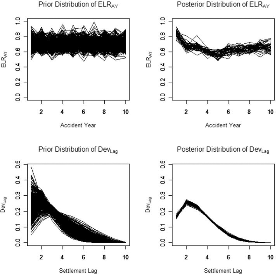
Note the autocorrelation in successive iterations resulting from the acceptance rates of around 25%. In an effort to minimize the effect of this autocorrelation, yet keep the sample manageably small for what follows, I selected a random sample of 1,000 iterations between t = 1,001 and t = 26,000 to represent the posterior distribution of parameters. Figures 7 and 8 are based on this sample.

Figure 7.Sample paths

Figure 8.Estimates
One way of viewing a Bayesian analysis is that one starts with a range of possible parameters, specified by the prior distribution. The posterior distribution can be thought of as a narrowing of the range implied by the data. Figure 7 illustrates this by plotting sample paths of {ELRAY} and {DevLag} for both the prior and posterior distributions.
For the Independent Factor model, I used the maximum likelihood estimates of the {DevLag} and {ELRAY} parameters as the starting values {DevLag}1 and {ELRAY}1. For the proposal density function, I used a gamma distribution, p(x∗∣xt−1)=Γ(x∗∣xt−1/αp,αp) with shape parameter αp=500 for x={ELRAY}. After some trial and error and examining trace plots similar to those in Figures 2-4, I concluded that the {DevLag} should vary by settlement lag, setting αp=2,000 times the maximum likelihood estimate of {DevLag}. Successive {DevLag}t and {ELRAY}t parameters were generated by the following simulation algorithm. As appropriate, g will denote the prior distributions of the parameters {DevLag} and {ELRAY}.
Simulation Algorithm 4
-
Select random candidate values, {DevLag}∗∗, from the proposal density function p({DevLag}∗∗∣{DevLag}t−1).
-
For each settlement lag, set Dev∗Lag=Dev∗∗Lag∑10i=1Dev∗∗i.
a. This step enforces the constraint that 10∑Lag=1DevLag=1.
-
Compute the ratio:
R=ℓ(X∣{ELRAY}t−1,{DevLag}∗)⋅g({DevLag}∗)⋅p({DevLag}t−1∣{DevLag}∗)(X∣{ELRAY}t−1,{DevLag}t−1)⋅g({DevLag}t−1)⋅p({DevLag}∗∣{DevLag}t−1).
-
Select a random number U from a uniform distribution on (0,1).
-
If U<R then set {DevLag}t={DevLag}∗. Otherwise set {DevLag}t={DevLag}t−1.
-
Select candidate values {ELRAY}∗ from the proposal density function p({ELRAY}∗ ∣{ELRAY}t−1).
-
Compute the ratio:
R=ℓ(X∣{ELRAY}∗,{DevLag}t)(g({ELRAY}∗)⋅p({ELRAY}t−1∣{ELRAY}∗)⋅(X∣{ELRAY}t−1,{DevLag}t)⋅g({ELRAY}t−1)⋅p({ELRAY}∗∣{ELRAY}t−1).
-
Select a random number U from a uniform distribution on (0,1).
-
If U<R then set {ELRAY}t={ELRAY}∗. Otherwise set {ELRAY}t={ELRAY}t−1.
I ran Simulation Algorithm 4 through 26,000 iterations. The acceptance rates for the {DevLag} and the {ELRAY} parameters were 24% and 27% respectively. As before, I selected a random sample of 1,000 iterations between t=1,001 and t= 26,000 to represent the posterior distribution of parameters. Figure 8 is based on this sample.
Computer code for implementing Simulation Algorithms 3 and 4, written in the R programming language, is included in Appendix C.
7. The distribution of estimates
Actuaries often use the term “range of reasonable estimates” to quantify the uncertainty in their estimation of a loss reserve. One source of this uncertainty comes from the statistical uncertainty of the parameter estimates, i.e., if one were to draw repeated random samples of data from the same underlying loss generating process, how variable would the estimate of the mean loss reserve be? Mack (1993) describes one popular way that actuaries use to quantify this uncertainty. This section describes a Bayesian analogue to the uncertainty that Mack quantifies.
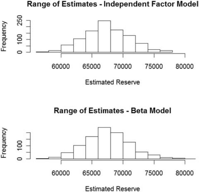
The last section provides samples of parameter estimates {ELRAY} and {DevLag} taken from the posterior distribution. For each record in the sample, calculate the estimated reserve as the sum of the expected loss in each (AY, Lag) cell for AY + Lag > 11.
E=10∑AY=2 Lag =12−AY Premium AY⋅ELRAY⋅ Dev Lag.
Figure 8 shows histograms of the estimates constructed from each record in the samples of the posterior distributions of {ELRAY} and {DevLag} for the beta and independent factor models.
The mean and standard deviation for these distributions of estimates are:
-
67,343,000 and 3,609,000 for the Independent Factor model; and
-
67,511,000 and 3,627,000 for the Beta model.
8. The predictive distribution of outcomes
Let’s now turn to the problem of predicting the sum of the future outcomes, XAY, Lag , when AY + Lag > 11 given in Table 7.
R=10∑AY=2Lag=12−AYX10AY, Lag .
| 1 |
50,000 |
7,168 |
11,190 |
12,432 |
7,856 |
3,502 |
1,286 |
334 |
216 |
190 |
0 |
| 2 |
50,000 |
4,770 |
8,726 |
9,150 |
5,728 |
2,459 |
2,864 |
715 |
219 |
0 |
X2,10 |
| 3 |
50,000 |
5,821 |
9,467 |
7,741 |
3,736 |
1,402 |
972 |
720 |
50 |
X3,9 |
X3,10 |
| 4 |
50,000 |
5,228 |
7,050 |
6,577 |
2,890 |
1,600 |
2,156 |
592 |
X4,8 |
X4,9 |
X4,10 |
| 5 |
50,000 |
4,185 |
6,573 |
5,196 |
2,869 |
3,609 |
1,283 |
X5,7 |
X5,8 |
X5,9 |
X5,10 |
| 6 |
50,000 |
4,930 |
8,034 |
5,315 |
5,549 |
1,891 |
X6,6 |
X6,7 |
X6,8 |
X6,9 |
X6,10 |
| 7 |
50,000 |
4,936 |
7,357 |
5,817 |
5,278 |
X7,5 |
X7,6 |
X7,7 |
X7,8 |
X7,9 |
X7,10 |
| 8 |
50,000 |
4,762 |
8,383 |
6,568 |
X8,4 |
X8,5 |
X8,6 |
X8,7 |
X8,8 |
X8,9 |
X8,10 |
| 9 |
50,000 |
5,025 |
8,898 |
X9,3 |
X9,4 |
X9,5 |
X9,6 |
X9,7 |
X9,8 |
X9,9 |
X9,10 |
| 10 |
50,000 |
4,824 |
X10,2 |
X10,3 |
X10,4 |
X10,5 |
X10,6 |
X10,7 |
X10,8 |
X10,9 |
X10,10 |
Suppose we have a set of parameters {ELRAY} and {DevLag } selected from iterations of a Met-ropolis-Hastings algorithm. Conceptually, the easiest way to calculate the distribution of outcomes is by repeated use of the following simulation algorithm.
Simulation Algorithm 5
-
Select the parameters {ELRAY} and {DevLag } from a randomly selected iteration.
-
For AY = 2, . . . ,10, do:
a. For Lag = 12 − AY to 10, do:
-
Set λAY, Lag =( Premium AY⋅ELRAY⋅DevLag)/(E[ZLag]).
-
Select N at random from a Poisson distribution with mean λAY,Lag.
-
If N>0, for i=1,…,N select claim amounts, Zi, Lag , at random from the claim severity distribution for the Lag.
-
If N>0, set XAY, Lag =∑Ni=1Zi, Lag , otherwise set XAY, Lag =0.
-
Set R=∑10AY=2∑10Lag=12−AYXAY, Lag .
I expect that many actuaries will be satisfied with using this simulation algorithm to calculate the predictive distribution. However, this paper uses an FFT to calculate the predictive distribution. While it is very technical and harder to implement, it is faster and it produces more accurate results (relative to the model assumptions). Appendix A describes how to implement the FFT for this paper’s application. Computer code implementing the FFT for calculating the predictive distributions in this paper, written in the R programming language, is included in Appendix C.
Figure 9 plots the density functions for the predictive distributions derived from the data in Table 7 and the parameters simulated as described in the last section.
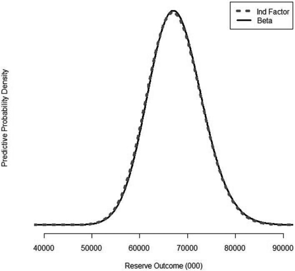
Figure 9.Density functions
The predictive means and standard deviations are:
-
67,343,000 and 5,677,000 for the Independent Factor model; and
-
67,511,000 and 5,685,000 for the Beta model.
The difference in the predictive means for the two models is 168,000 or 0.25%. This is not terribly surprising in light of the fact that the data was simulated from a model where the {DevLag} parameters were randomly selected from a beta distribution. It appears, in this case anyway, that not much in the way of predictive accuracy was lost by using the Independent Factor model with its additional parameters.
9. Conclusion
While this paper does contain some new material, I made an attempt to write it as an expository paper. By considering two models, the Independent Factor model and the Beta model, it should be clear that the Metropolis-Hastings algorithm could be applied to other models. For example:
-
One could force a constraint so that the last three {DevLag} parameters decrease by a constant factor.
-
If a claim severity distribution was not available, one could use the Tweedie distribution and treat the τ and/or p parameters as unknown.
-
One could use the full collective risk model by calculating the log-likelihood with the FFT as done in Meyers (2007).
Appendix
This paper describes the collective risk model in terms of a simulation algorithm. Given the speed of today’s personal computers, it is practical to actually do the simulations in a reasonable amount of time. This appendix describes how to do many of the calculations to a higher degree of accuracy in a significantly shorter time using FFTs.
The advantage to using FFTs is that the time-consuming task of calculating the distribution of the sum of random variables is transformed into the much faster task of multiplying the FFTs of the distributions. Simulation Algorithms 1 and 5 show that the collective risk model requires the calculation of the distribution of the sum of random claim amounts. Furthermore, Simulation Algorithm 5 requires the calculation of the distribution of the sum of losses over different accident years and settlement lags.
This appendix has three sections. Since the FFTs work on discrete random variables, the first section shows how to discretize the claim severity distribution in such a way that the limited average severities of the continuous severity distribution are preserved. The second section will show how to calculate the probabilities associated with the collective risk model. The third section will show how to calculate the predictive distribution for the outstanding losses.
A.1. Discretizing the claim severity distributions
The first step is to determine the discretization interval length h. Length h, which depended on the size of the insurer, was chosen so the 214 (16,384) values spanned the probable range of annual losses for the insurer. Specifically, let h1 be the sum of the insurer’s 10-year premium divided by 214. The h was set equal to 1,000 times the smallest number from the set {5, 10, 20, 25, 40, 50, 100, 125, 200, 250, 500, 1000} that was greater than h1 / 1000. This last step guarantees that a multiple, m, of h would be equal to the policy limit of 1,000,000.
The next step is to use the mean-preserving method (described in Klugman, Panjer, and Willmot 2004, p. 656) to discretize the claim severity distribution for each settlement lag. Let pi, Lag represent the probability of a claim with severity h⋅i for each settlement lag. Using the limited average severity (LASLag) function determined from claim severity distributions, the method proceeds in the following steps.
- p0, Lag =1−LASLag(h)/h.
- pi, Lag =(2⋅LASLag(h⋅i)−LASLag(h⋅(i−1)) −LASLag(h⋅(i+1)))/h for i=1,2,…,m−1.
- pm, Lag =1−∑m−1i=0pi, Lag .
- pik=0 for i=m+1,…,214−1.
A.2. Calculating probabilities for the compound Poisson distribution
The purpose of this section is to show how to calculate the probabilities of losses defined by the collective risk model as defined in Simulation Algorithm 1. The math described in this section is derived in Klugman, Panjer, and Willmot (2004, Section 6.91). The calculation proceeds in the following steps.
-
Set →pLag={p0, Lag ,…p214−1, Lag }.
-
Calculate the expected claim count, λAY,Lag, for each accident year and settlement lag using Equation 2, λAY, Lag ≡E[ Paid LossAY, Lag ]/E[ZLag].
-
Calculate the FFT of →pLag,Φ(→pLag).
-
Calculate the FFT of each aggregate loss random variable, XAY,Lag, using the formula Φ(→qAY, Lag )=eλ(Φ(→pLag)−1). This formula is derived in Klugman, Panjer, and Willmot (2004, Section 6.91).
-
Calculate →qAY, Lag =Φ−1(Φ(→qAY, Lag )), the inverse FFT of the expression in Step 4.
The vector, →qAY,Lag , contains the probabilities of the discretized compound Poisson distribution defined by Simulation Algorithm 1.
A.3. Calculating probabilities for the predictive distribution
To calculate the predictive distribution of the reserve outcomes by the methods in this paper, one needs the {ELRAY,DevLag} parameter set that was simulated by the Metropolis-Hastings algorithm as described in Section 6.
-
For each parameter set, denoted by i, and AY+Lag>11, do the following:
a. Calculate the expected loss, PremiumAY,i. ELRAY,i⋅DevLag,i.
b. Calculate the FFT of the aggregate loss XAY,Lag,i,Φ(→qAY,Lag,i) as described in Step 4 in Section A.2.
-
For each parameter set, i, calculate the product Φ(→qi)≡∏10AY=2∏10Lag=12−AYΦ(→qAY, Lag ,i).
-
Calculate the FFT of the mixture over all i, Φ(→q)=(∑iΦ(→qi)/n), where n is the number of Metropolis samples used in the posterior distribution.
-
Invert the FFT, Φ(→q), to obtain the vector, →q, which describes the distribution of the reserve outcomes.
Here are the formulas to calculate the mean and standard deviation of the reserve outcomes:
- Expected Value =h⋅∑214−1j=0j⋅→qj.
- Second Moment =h2⋅∑214−1j=0j2⋅→qj.
- Standard Deviation =√ Second Moment −( First Moment )2.
Figure 9 has plots of the →q s for the Cape Cod and the Beta models.
Appendix B. A fast approximation of the Tweedie distribution
The goal of this appendix is to show how to calculate approximate likelihoods ℓ(X∣{ELRAY}, {DevLag } ) for the independent factor model and ℓ(X∣{ELRAY},a,b) for the beta model, where the distribution of each XAY, Lag is approximated by a Tweedie distribution as described in Section 3 above.
Peter Dunn has written a package for the R programming language that calculates various functions associated with the Tweedie distribution. The methods of calculation are described in Dunn and Smyth (2008). Our particular interest is in the density function.
The model dispersion form of the Tweedie density function, as given by Dunn and Smyth (2008), is written as follows.
f(y∣p,μ,ϕ)=f(y∣p,y,ϕ)⋅exp(−12ϕd(y,μ)),
where the deviance function, d(y,μ) is given by:
d(y,μ)=2⋅(y2−p(1−p)⋅(2−p)−y⋅μ1−p1−p+μ2−p2−p).
Standard statistical procedures, such as the “glm” function in R, will fit a Tweedie model by maximum likelihood. These models assume that μ is a linear function of independent variables, {xi}, with unknown coefficients, {βi}. The parameters ϕ and p are assumed to be known and constant. This is particularly convenient since the function f(y∣p,y,ϕ) is not of closed form and takes relatively long to compute. The deviance function, d(y,μ), that contains all of the unknown parameters, is of closed form and can be calculated quickly.
Now let’s examine how this paper makes use of the Tweedie distribution. First it finds the first two limited moments, m1, Lag and m2, Lag , of the Pareto claim severity distributions. Using these moments it calculates the shape parameters, αLag =m2, Lag /m21, Lag −1. Then by Equation 4 in the main text, pLag=(αLag+2)/(αLag+1). It is worth noting that the pLags are between 1.6 and 1.9.
Next we set μAY,Lag=PremiumAY⋅ELRAY. DevLag and set ϕAY, Lag =(μ1−pAY, Lag ⋅m1, Lag )/(2−pLag).
At this point, it is important to examine how the Tweedie package in R, written by Peter Dunn of Dunn and Smyth (2008), works. Each call to the density function “dtweedie” invokes the long calculation, f(y \mid p, y, \phi) in Equation B.1. Once that function is called, the length of the vectors p, y, and \phi add little to the computing time.
The Metropolis-Hastings algorithms used in this paper call for an evaluation of the Tweedie density function twice in each iteration. When thousands of iterations are necessary, computing speed becomes important.
This paper uses a closed-form approximation of log(f(y | p,y,ϕ)) to speed up the calculation. Here is how it works. Dunn and Smyth (2008) give a useful transformation:
f(y \mid p, \mu, \phi)=k \cdot f\left(k y \mid p, k \mu, k^{2-p} \phi\right) . \tag{B.3}
By setting k=\phi^{-1 /(2-p)} we have f(y \mid p, y, \phi) =k \cdot f(k y \mid p, k y, 1). For each p_{\text {Lag}}, all we need is an approximation for f\left(y \mid p_{\text {Lag}}, y, 1\right). It turns out that for 1 \ll p<2, \log \left(f\left(y \mid p_{\text {Lag}}, y, 1\right)\right) can be accurately approximated by a cubic polynomial of the form a_0+a_1 x+a_2 x^2+a_3 x^3. Tables B. 1 and B. 2 show the coefficients of the cubic approximation and the accuracy for selected values of p.
Table B.1.Coefficients of the cubic approximation
| 1.05 |
−1.0537298 |
−0.4495751 |
−0.0075734 |
−0.0007098 |
| 1.10 |
−1.0075666 |
−0.4943442 |
−0.0109068 |
0.0006014 |
| 1.15 |
−1.0030623 |
−0.5213300 |
−0.0118162 |
0.0008680 |
| 1.20 |
−1.0056630 |
−0.5444444 |
−0.0128532 |
0.0010362 |
| 1.25 |
−1.0111141 |
−0.5653465 |
−0.0144145 |
0.0012391 |
| 1.30 |
−1.0166456 |
−0.5869880 |
−0.0155553 |
0.0013820 |
| 1.35 |
−1.0211424 |
−0.6105617 |
−0.0158944 |
0.0014264 |
| 1.40 |
−1.0243110 |
−0.6362369 |
−0.0154279 |
0.0013765 |
| 1.45 |
−1.0261726 |
−0.6637913 |
−0.0142951 |
0.0012522 |
| 1.50 |
−1.0268557 |
−0.6928798 |
−0.0126759 |
0.0010777 |
| 1.55 |
−1.0265187 |
−0.7231318 |
−0.0107539 |
0.0008763 |
| 1.60 |
−1.0253224 |
−0.7541853 |
−0.0087030 |
0.0006698 |
| 1.65 |
−1.0234203 |
−0.7856997 |
−0.0066798 |
0.0004764 |
| 1.70 |
−1.0209541 |
−0.8173670 |
−0.0048178 |
0.0003104 |
| 1.75 |
−1.0180503 |
−0.8489231 |
−0.0032184 |
0.0001809 |
| 1.80 |
−1.0148165 |
−0.8801616 |
−0.0019442 |
0.0000906 |
| 1.85 |
−1.0113387 |
−0.9109414 |
−0.0010153 |
0.0000363 |
| 1.90 |
−1.0076816 |
−0.9411858 |
−0.0004133 |
0.0000099 |
| 1.95 |
−1.0038912 |
−0.9708695 |
−0.0000938 |
0.0000011 |
Table B.2.Summary statistics for error
| p |
Min |
1st Quart. |
Median |
Mean |
3rd Quart. |
Max |
| 1.05 |
−0.5809000 |
−0.0089460 |
−0.0014980 |
0.0000000 |
0.0116600 |
0.5771000 |
| 1.10 |
−0.1134000 |
−0.0020520 |
0.0000026 |
0.0000000 |
0.0035110 |
0.1815000 |
| 1.15 |
−0.0272000 |
−0.0007594 |
0.0001503 |
0.0000000 |
0.0016800 |
0.0567600 |
| 1.20 |
−0.0073860 |
−0.0003781 |
0.0000727 |
0.0000000 |
0.0007142 |
0.0171100 |
| 1.25 |
−0.0019210 |
−0.0003373 |
0.0000251 |
0.0000000 |
0.0003417 |
0.0036560 |
| 1.30 |
−0.0012350 |
−0.0003801 |
0.0000048 |
0.0000000 |
0.0004188 |
0.0006517 |
| 1.35 |
−0.0026570 |
−0.0004858 |
0.0000608 |
0.0000000 |
0.0005484 |
0.0008492 |
| 1.40 |
−0.0027840 |
−0.0005010 |
0.0000517 |
0.0000000 |
0.0005574 |
0.0009526 |
| 1.45 |
−0.0023540 |
−0.0004498 |
0.0000433 |
0.0000000 |
0.0004966 |
0.0008563 |
| 1.50 |
−0.0017590 |
−0.0003617 |
0.0000347 |
0.0000000 |
0.0003991 |
0.0006697 |
| 1.55 |
−0.0011890 |
−0.0002627 |
0.0000256 |
0.0000000 |
0.0002908 |
0.0004689 |
| 1.60 |
−0.0007282 |
−0.0001717 |
0.0000170 |
0.0000000 |
0.0001910 |
0.0002951 |
| 1.65 |
−0.0003994 |
−0.0000998 |
0.0000100 |
0.0000000 |
0.0001115 |
0.0001654 |
| 1.70 |
−0.0001921 |
−0.0000504 |
0.0000051 |
0.0000000 |
0.0000565 |
0.0000809 |
| 1.75 |
−0.0000782 |
−0.0000213 |
0.0000022 |
0.0000000 |
0.0000240 |
0.0000334 |
| 1.80 |
−0.0000254 |
−0.0000071 |
0.0000007 |
0.0000000 |
0.0000080 |
0.0000109 |
| 1.85 |
−0.0000061 |
−0.0000017 |
0.0000002 |
0.0000000 |
0.0000019 |
0.0000026 |
| 1.90 |
−0.0000008 |
−0.0000002 |
0.0000000 |
0.0000000 |
0.0000003 |
0.0000004 |
| 1.95 |
0.0000000 |
0.0000000 |
0.0000000 |
0.0000000 |
0.0000000 |
0.0000000 |
The software that calculates the log-likelihood for the Tweedie starts by calling dtweedie ( y, p_{\text {Lag}}, y, 1 ) once for each value of p_{\text {Lag}} for a long vector y. It then uses a simple linear regression to calculate the cubic polynomial that best approximates \log \left(f\left(y \mid p_{\text {Lag}}, y, 1\right)\right). It then uses that polynomial in Equation B. 1 in place of \log \left(f\left(y \mid p_{\text {Lag}}, y, 1\right)\right) when calculating the loglikelihood thousands of times.
Appendix C. Computer code for the algorithms
This appendix describes the code that implements the algorithms in this paper. The code is written in R, a computer language that can be downloaded for free at www.R-Project.org.
-
The Rectangle.csv-This is the triangle in Table 1 expressed in rectangular form so it fits into an R data frame.
-
Ind Factor Model Posterior.r—This code reads The Rectangle.csv and implements the Met-ropolis-Hastings algorithm to produce an output file, Ind Factor Posterior.csv, containing sampled \left\{E L R_{A Y}\right\} and \left\{D e v_{\text {Lag }}\right\} parameters from the Independent Factor model.
-
Beta Model Posterior.r-This code reads The Rectangle.csv and implements the MetropolisHastings algorithm to produce an output file, Beta Posterior.csv, containing sampled \left\{E L R_{A Y}\right\} and \left\{D e v_{L a g}\right\} parameters from the beta model.
-
Estimates and Predicted Outcomes.r —This code takes the either of the output files the code described above and calculates the distribution of the estimates and the predictive distribution. It creates graphs like those in Figures 8 and 9.
The Rectangle.csv
| 50000 |
1 |
1 |
7168 |
| 50000 |
1 |
2 |
11190 |
| 50000 |
1 |
3 |
12432 |
| 50000 |
1 |
4 |
7856 |
| 50000 |
1 |
5 |
3502 |
| 50000 |
1 |
6 |
1286 |
| 50000 |
1 |
7 |
334 |
| 50000 |
1 |
8 |
216 |
| 50000 |
1 |
9 |
190 |
| 50000 |
1 |
10 |
0 |
| 50000 |
2 |
1 |
4770 |
| 50000 |
2 |
2 |
8726 |
| 50000 |
2 |
3 |
9150 |
| 50000 |
2 |
4 |
5728 |
| 50000 |
2 |
5 |
2459 |
| 50000 |
2 |
6 |
2864 |
| 50000 |
2 |
7 |
715 |
| 50000 |
2 |
8 |
219 |
| 50000 |
2 |
9 |
0 |
| 50000 |
3 |
1 |
5821 |
| 50000 |
3 |
2 |
9467 |
| 50000 |
3 |
3 |
7741 |
| 50000 |
3 |
4 |
3736 |
| 50000 |
3 |
5 |
1402 |
| 50000 |
3 |
6 |
972 |
| 50000 |
3 |
7 |
720 |
| 50000 |
3 |
8 |
50 |
| 50000 |
4 |
1 |
5228 |
| 50000 |
4 |
2 |
7050 |
| 50000 |
4 |
3 |
6577 |
| 50000 |
4 |
4 |
2890 |
| 50000 |
4 |
5 |
1600 |
| 50000 |
4 |
6 |
2156 |
| 50000 |
4 |
7 |
592 |
| 50000 |
5 |
1 |
4185 |
| 50000 |
5 |
2 |
6573 |
| 50000 |
5 |
3 |
5196 |
| 50000 |
5 |
4 |
2869 |
| 50000 |
5 |
5 |
3609 |
| 50000 |
5 |
6 |
1283 |
| 50000 |
6 |
1 |
4930 |
| 50000 |
6 |
2 |
8034 |
| 50000 |
6 |
3 |
5315 |
| 50000 |
6 |
4 |
5549 |
| 50000 |
6 |
5 |
1891 |
| 50000 |
7 |
1 |
4936 |
| 50000 |
7 |
2 |
7357 |
| 50000 |
7 |
3 |
5817 |
| 50000 |
7 |
4 |
5278 |
| 50000 |
8 |
1 |
4762 |
| 50000 |
8 |
2 |
8383 |
| 50000 |
8 |
3 |
6568 |
| 50000 |
9 |
1 |
5025 |
| 50000 |
9 |
2 |
8898 |
| 50000 |
10 |
1 |
4824 |
Ind Factor Model Posterior.r
# Code for calculating the factor model posterior in
# "Stochastic Loss Reserving with the Collective Risk Model"
#
# Inputs
#
set.seed(12345)
nmh=26000 # size
mh.out="Ind Factor Posterior.csv"
#
# get loss data
#
rdata=read.csv("The Rectangle.csv")
#
# create loss distribution
#
limit=1000
theta=c(10,25,50,75,100,125,150,150,150,150)
alpha=rep(2,10)
#
# prior distribution
#
alpha.elr=100
theta.elr=0.007
alpha.dev=c(11.0665,64.4748,189.6259,34.8246,10.6976, 4.4824, 2.1236, 1.0269, 0.4560, 0.1551)
theta.dev=c(.0206,.0041,.0011,.0040,.0079,.0101,.0097,.0073,.0039,.0009)
#
########################### Begin Subprograms ###########################
#
# Get the b(y,1) function from Dunn and Smyth
#
lltweedie.front=function(y,cc,k){
x1=log(y)
x2=x1^ 2
x3=x1^ 3
lf=cc[k,1]+cc[k,2]*x1+cc[k,3]*x2+cc[k,4]*x3
return(lf)
}
# get tweedie loglikelihood using the Dunn and Smyth scale transform
#
lltweedie.scaled=function(y,p,mu,phi,k1){
dev=y
ll=y
k=(1/phi)^ (1/(2-p[k1]))
ky=k*y
yp=y> 0
dev[yp]=2*((k[yp]*y[yp])^ (2-p[k1[yp]])/((1-p[k1[yp]])*(2-p[k1[yp]]))-
k[yp]*y[yp]*(k[yp]*mu[yp])^ (1-p[k1[yp]])/(1-p[k1[yp]])+
(k[yp]*mu[yp])^ (2-p[k1[yp]])/(2-p[k1[yp]]))
ll[yp]=log(k[yp])+lltweedie.front(ky[yp],cubic.coef,k1[yp])-dev[yp]/2
ll[!yp]=-mu[!yp]^ (2-p[k1[!yp]])/phi[!yp]/(2-p[k1[!yp]])
return(ll)
}
#
# Pareto limited average severity
#
pareto.las=function(x,theta,alpha){
las= ifelse(alpha==1,-theta*log(theta/(x+theta)),
theta/(alpha-1)*(1-(theta/(x+theta))^ (alpha-1)))
return(las)
}
#
# Pareto limited second moment
#
pareto.m2=function(x,th,al){
den=x^ 2*al*th^ al/(x+th)^ (al+1)
return(den)
}
#
pareto.lsm=function(x,theta,alpha){
lsm=integrate(pareto.m2,0,x,th=theta,al=alpha)$value+
x*x*(theta/(x+theta))^ alpha
return(lsm)
}
#
# tdev to dev function
#
tdev.to.dev=function(tdev){
dev=1:10
dev[1]=exp(-tdev[1]^ 2)
cp=1
for (i in 2:10){
cp=cp*(1-dev[i-1])
dev[i]=cp*exp(-tdev[i]^ 2)
}
dev=pmax(dev,0.0001) # fix for when any of the tdevs are very small.
dev=dev/sum(dev)
return(dev)
}
#
# factor crm log-likelihood
#
fact.crm.llike0.tdev=function(dev.elr){
dev=tdev.to.dev(dev.elr[1:10])
elr=dev.elr[11:20]
eloss=rdata$premium*dev[rdata$lag]*elr[rdata$ay]
phi=eloss^ (1-tweedie.p[rdata$lag])*esev[rdata$lag]/(2-tweedie.p[rdata$lag])
llike=lltweedie.scaled(rdata$loss,tweedie.p,eloss,phi,rdata$lag)
return(sum(llike))
}
#
# factor crm likelihood
#
fact.crm.llike1=function(dev,elr){
eloss=rdata$premium*dev[rdata$lag]*elr[rdata$ay]
phi=eloss^ (1-tweedie.p[rdata$lag])*esev[rdata$lag]/(2-tweedie.p[rdata$lag])
llike1=lltweedie.scaled(rdata$loss,tweedie.p,eloss,phi,rdata$lag)
return(sum(llike1))
}
#
# log prior
#
log.prior=function(dev,elr){
d=dgamma(dev,alpha.dev,scale=theta.dev,log=T)
e=dgamma(elr,alpha.elr,scale=theta.elr,log=T)
return(sum(d,e))
}
log.proposal.den=function(x,m,alpha){
d=dgamma(x,alpha,scale=m/alpha,log=T)
return(sum(d))
}
#
# Begin main program ###########################################################
#
library(tweedie)
ytop=100
y1=seq(from=ytop/100000,to=ytop,length=100000)
x1=log(y1)
x2=x1^ 2
x3=x1^ 3
cubic.coef=matrix(NA,10,4)
#
# initialize variables
#
esev=rep(0,10)
elsm=rep(0,10)
tweedie.p=1:10
for (k in 1:10){
esev[k]=pareto.las(limit,theta[k],alpha[k])
elsm[k]=pareto.lsm(limit,theta[k],alpha[k])
cvsq=elsm[k]/esev[k]^ 2-1
tweedie.p[k]=(1+2*cvsq)/(1+cvsq)
front=dtweedie(y1,tweedie.p[k],y1,1)
af=lm(log(front)~x1+x2+x3)
cubic.coef[k,]=af$coefficients
} #end k loop
#alpha=esev[rdata$lag]^ 2/(elsm[rdata$lag]-esev[rdata$lag]^ 2)
mh.dev=matrix(0,nmh,10)
mh.elr=matrix(0,nmh,10)
#
# produce a posterior distribution of parameters using the MH algorithm
#
# find maximum likelihood estimate
#
ml=optim(c(rep(1,10),rep(.7,10)),fact.crm.llike0.tdev,
control=list(fnscale=-1,maxit=25000))
devg=tdev.to.dev(ml$par[1:10])
elrg=ml$par[11:20]
mh.dev[1,]=devg
mh.elr[1,]=elrg
prev.log.post=ml$value+log.prior(devg,elrg)
#
# produce a sample of (dev,elr) parameters from the posterior distribution
#
alpha.prop.dev=2000*devg
alpha.prop.elr=500
accept.dev=0
accept.elr=0
for (i in 2:nmh){
devg=rgamma(10,shape=alpha.prop.dev[1:10],
scale=mh.dev[i-1,1:10]/alpha.prop.dev[1:10])
devg=devg/sum(devg)
u=log(runif(1))
log.post=fact.crm.llike1(devg,mh.elr[i-1,])+log.prior(devg,mh.elr[i-1,])
r=log.post-prev.log.post+log.proposal.den(mh.dev[i-1,],devg,alpha.prop.dev)-
log.proposal.den(devg,mh.dev[i-1,],alpha.prop.dev)
mh.dev[i,]=mh.dev[i-1,]
if(u< r){
mh.dev[i,]=devg
accept.dev=accept.dev+1
prev.log.post=log.post
}
#
elrg=rgamma(10,shape=alpha.prop.elr,scale=mh.elr[i-1,]/alpha.prop.elr)
u=log(runif(1))
log.post=fact.crm.llike1(mh.dev[i,],elrg)+log.prior(mh.dev[i,],elrg)
r=log.post-prev.log.post+log.proposal.den(mh.elr[i-1,],elrg,alpha.prop.elr)-
log.proposal.den(elrg,mh.elr[i-1,],alpha.prop.elr)
mh.elr[i,]=mh.elr[i-1,]
if(u< r){
mh.elr[i,]=elrg
accept.elr=accept.elr+1
prev.log.post=log.post
}
}
#
# MCMC convergence diagnostics
#
library(stats)
windows(record=T)
par(mfrow=c(2,1)) for (i in 1:10){
Dev=mh.dev[,i]
plot(1:nmh,Dev,main=paste("Development Factor for Lag ",i),type="l",
xlab="Iteration")
abline(mh.dev[1,i],0,lwd=3)
temp=acf(Dev,lwd=3)
}
for (i in 1:10){
ELR=mh.elr[,i]
plot(1:nmh,ELR,main=paste("Expected Loss Ratio for AY ",i),type="l",
xlab="Iteration")
abline(mh.elr[1,i],0,lwd=3)
temp=acf(ELR,lwd=3)
}
#
# take a sample and write to an output file
#
s=sample(1001:nmh,1000)
posterior=data.frame(mh.elr[s,],mh.dev[s,])
names(posterior)=c("ELR1","ELR2","ELR3","ELR4","ELR5","ELR6","ELR7",
"ELR8","ELR9","ELR10","Lag1","Lag2","Lag3","Lag4",
"Lag5","Lag6","Lag7","Lag8","Lag9","Lag10")
write.csv(posterior,file=mh.out,row.names=F)
#
# write out acceptance rates at the end
#
100*accept.dev/nmh
100*accept.elr/nmh
Beta Model Posterior.r
# Code for calculating the beta model posterior in
# "Stochastic Loss Reserving with the Collective Risk Model"
#
# Inputs
#
set.seed(12345)
nmh=26000 # size
mh.out="Beta Posterior.csv"
#
# get loss data #
rdata=read.csv("The Rectangle.csv")
#
# create loss distribution #
limit=1000
theta=c(10,25,50,75,100,125,150,150,150,150)
alpha=rep(2,10)
#
# prior distribution
#
alpha.elr=100
theta.elr=0.007
alpha.a=75
theta.a=.02
alpha.b=25
theta.b=.2
#
######################### Begin Subprograms ####################################
#
# Get the b(y,1) function from Dunn and Smyth
#
lltweedie.front=function(y,cc,k){
x1=log(y)
x2=x1^ 2
x3=x1^ 3
lf=cc[k,1]+cc[k,2]*x1+cc[k,3]*x2+cc[k,4]*x3
return(lf)
}
# get tweedie loglikelihood using the Dunn and Smyth scale transform
#
lltweedie.scaled=function(y,p,mu,phi,k1){
dev=y
ll=y
k=(1/phi)^ (1/(2-p[k1]))
ky=k*y
yp=y> 0
dev[yp]=2*((k[yp]*y[yp])^ (2-p[k1[yp]])/((1-p[k1[yp]])*(2-p[k1[yp]]))-
k[yp]*y[yp]*(k[yp]*mu[yp])^ (1-p[k1[yp]])/(1-p[k1[yp]])+
(k[yp]*mu[yp])^ (2-p[k1[yp]])/(2-p[k1[yp]]))
ll[yp]=log(k[yp])+lltweedie.front(ky[yp],cubic.coef,k1[yp])-dev[yp]/2
ll[!yp]=-mu[!yp]^ (2-p[k1[!yp]])/phi[!yp]/(2-p[k1[!yp]])
return(ll)
}
#
# Pareto limited average severity
#
pareto.las=function(x,theta,alpha){
las= ifelse(alpha==1,-theta*log(theta/(x+theta)),
theta/(alpha-1)*(1-(theta/(x+theta))^ (alpha-1)))
return(las)
}
#
# Pareto limited second moment
#
pareto.m2=function(x,th,al){
den=x^ 2*al*th^ al/(x+th)^ (al+1)
return(den)
}
#
pareto.lsm=function(x,theta,alpha){
lsm=integrate(pareto.m2,0,x,th=theta,al=alpha)$value+
x*x*(theta/(x+theta))^ alpha
return(lsm)
}
#
# beta generated cnm likelihood using nb approximation
#
beta.crm.llike0=function(a.b.elr){
a=a.b.elr[1]
b=a.b.elr[2]
elr=a.b.elr[3:12]
cdev1=pbeta((1:10)/10,a,b)
dev=cdev1-c(0,cdev1[-10])
eloss=rdata$premium*dev[rdata$lag]*elr[rdata$ay]
phi=eloss^ (1-tweedie.p[rdata$lag])*esev[rdata$lag]/(2-tweedie.p[rdata$lag])
llike=lltweedie.scaled(rdata$loss,tweedie.p,eloss,phi,rdata$lag)
return(sum(llike))
}# end beta.crm.llike0.approx
#
# factor crm likelihood
#
fact.crm.llike1=function(dev,elr){
eloss=rdata$premium*dev[rdata$lag]*elr[rdata$ay]
phi=eloss^ (1-tweedie.p[rdata$lag])*esev[rdata$lag]/(2-tweedie.p[rdata$lag])
llike1=lltweedie.scaled(rdata$loss,tweedie.p,eloss,phi,rdata$lag)
return(sum(llike1))
}
#
# log prior
#
log.prior=function(a.b,elr){
a=dgamma(a.b[1],alpha.a,scale=theta.a,log=T)
b=dgamma(a.b[2],alpha.b,scale=theta.b,log=T)
e=dgamma(elr,alpha.elr,scale=theta.elr,log=T)
return(sum(a,b,e))
}
log.proposal.den=function(x,m,alpha){
d=dgamma(x,alpha,scale=m/alpha,log=T)
return(sum(d))
}
#
# Begin main program ###########################################################
#
library(statmod)
library(tweedie)
ytop=100
y1=seq(from=ytop/100000,to=ytop,length=100000)
x1=log(y1)
x2=x1^ 2
x3=x1^ 3
cubic.coef=matrix(NA,10,4)
#
# initialize variables
#
esev=rep(0,10)
elsm=rep(0,10
tweedie.p=1:10
for (k in 1:10){
esev[k]=pareto.las(limit,theta[k],alpha[k])
elsm[k]=pareto.lsm(limit,theta[k],alpha[k])
cvsq=elsm[k]/esev[k]^ 2-1
tweedie.p[k]=(1+2*cvsq)/(1+cvsq)
front=dtweedie(y1,tweedie.p[k],y1,1)
af=lm(log(front) x1+x2+x3)
cubic.coef[k,]=af$coefficients
} #end k loop
mh.a.b=matrix(0,nmh,2)
mh.dev=matrix(0,nmh,10)
mh.elr=matrix(0,nmh,10)
#
# produce a posterior distribution of parameters using the MH algorithm
#
# find maximum likelihood estimate
#
ml=optim(c(alpha.a*theta.a,alpha.b*theta.b,1,rep(.7,10)),beta.crm.llike0,
control=list(fnscale=-1,maxit=25000))
a.bg=ml$par[1:2]
cdev1=pbeta((1:10)/10,a.bg[1],a.bg[2])
devg=cdev1-c(0,cdev1[-10])
elrg=ml$par[3:12]
mh.a.b[1,]=a.bg
mh.dev[1,]=devg mh.elr[1,]=elrg
prev.log.post=ml$value+log.prior(devg,elrg)
#
# produce a sample of (dev,elr) parameters from the posterior distribution
#
alpha.prop.a.b=500
alpha.prop.elr=500
accept.dev=0
accept.elr=0
for (i in 2:nmh){
a.bg=rgamma(2,shape=alpha.prop.a.b,
scale=mh.a.b[i-1,]/alpha.prop.a.b)
cdev1=pbeta((1:10)/10,a.bg[1],a.bg[2])
devg=cdev1-c(0,cdev1[-10])
u=log(runif(1))
log.post=fact.crm.llike1(devg,mh.elr[i-1,])+log.prior(a.bg,mh.elr[i-1,])
r=log.post-prev.log.post+log.proposal.den(mh.a.b[i-1,],a.bg,alpha.prop.a.b)-
log.proposal.den(a.bg,mh.a.b[i-1,],alpha.prop.a.b)
mh.a.b[i,]=mh.a.b[i-1,]
mh.dev[i,]=mh.dev[i-1,]
if(u< r){
mh.a.b[i,]=a.bg
mh.dev[i,]=devg
accept.dev=accept.dev+1
prev.log.post=log.post
}
#
elrg=rgamma(10,shape=alpha.prop.elr,scale=mh.elr[i-1,]/alpha.prop.elr)
u=log(runif(1))
log.post=fact.crm.llike1(mh.dev[i,],elrg)+log.prior(mh.a.b[i,],elrg)
r=log.post-prev.log.post+log.proposal.den(mh.elr[i-1,],elrg,alpha.prop.elr)-
log.proposal.den(elrg,mh.elr[i-1,],alpha.prop.elr)
mh.elr[i,]=mh.elr[i-1,]
if(u< r){
mh.elr[i,]=elrg
accept.elr=accept.elr+1
prev.log.post=log.post
}
}
#
# MCMC convergence diagnostics
#
library(stats)
windows(record=T)
par(mfrow=c(2,1))
for (i in 1:10){
Dev=mh.dev[,i]
plot(1:nmh,Dev,main=paste("Development Factor for Lag ",i),type="l",
xlab="Iteration")
abline(mh.dev[1,i],0,lwd=3)
temp=acf(Dev,lwd=3)
}
for (i in 1:10){
ELR=mh.elr[,i]
plot(1:nmh,ELR,main=paste("Expected Loss Ratio for AY ",i),type="l",
xlab="Iteration")
abline(mh.elr[1,i],0,lwd=3)
temp=acf(ELR,lwd=3)
}
#
# take a sample and write to an output file
#
s=sample(1001:nmh,1000)
posterior=data.frame(mh.elr[s,],mh.dev[s,])
names(posterior)=c("ELR1","ELR2","ELR3","ELR4","ELR5","ELR6","ELR7",
"ELR8","ELR9","ELR10","Lag1","Lag2","Lag3","Lag4",
"Lag5","Lag6","Lag7","Lag8","Lag9","Lag10")
write.csv(posterior,file=mh.out,row.names=F)
#
# write out acceptance rates at the end
#
100*accept.dev/nmh
100*accept.elr/nmh
Estimates and Predicted Outcomes.r
# Code for calculating the predictive distribution in
# "Stochastic Loss Reserving with the Collective Risk Model"
#
# input premium=rep(50000,10)
post.input="Beta Posterior.csv"
#
# estimate the step size for discrete loss distribution
#
estimate.h< -function(premium,fftn,limit.divisors){
h< -10*premium/2^ fftn
h< -min(subset(limit.divisors,limit.divisors> h))
return(h)
}
#
# Pareto limited average severity
#
pareto.las< -function(x,theta,alpha){
las< - ifelse(alpha==1,-theta*log(theta/(x+theta)),
theta/(alpha-1)*(1-(theta/(x+theta))^ (alpha-1)))
return(las)
}
#
# total reserve predictive distribution
#
totres.predictive.dcnb=function(prem,elr,dev,esev,dp,phiz){
phix=complex(2^ fftn,0,0)
for (i in 1:npost){
phixp=complex(2^ fftn,1,0)
for (j in 2:10){
dpp=rep(0,2^ fftn)
lamp=0
for (k in (12-j):10) {
eloss=prem[j]*elr[i,j]*dev[i,k]
lam=eloss/esev[k]
lamp=lamp+lam
dpp=dpp+dp[,k]*lam
} # end k loop
dpp=dpp/lamp
phixp=phixp*exp(lamp*(fft(dpp)-1))
} # end j loop
phix=phix+phixp
} # end i loop
pred=round(Re(fft(phix/npost,inverse=TRUE)),12)/2^ fftn
return(pred)
} #end totres predictive densityposterior=read.csv("beta_posterior.csv")
#
# discretized Pareto severity distribution
#
discrete.pareto< -function(limit,theta,alpha,h,fftn){
dpar< -rep(0,2^ fftn)
m< -ceiling(limit/h)
x< -h*0:m
las< -rep(0,m+1)
for (i in 2:(m+1)) {
las[i]< -pareto.las(x[i],theta,alpha)
} #end i loop
dpar[1]< -1-las[2]/h
dpar[2:m]< -(2*las[2:m]-las[1:(m-1)]-las[3:(m+1)])/h
dpar[m+1]< -1-sum(dpar[1:m])
return(dpar)
} # end discrete.pareto function
#
# begin main program
#
# set up severity distribution
#
posterior=read.csv(post.input)
range=1:dim(posterior)[1]
elr=as.matrix(posterior)[range,1:10]
dev=as.matrix(posterior)[range,11:20]
npost=dim(elr)[1]
fftn< -14
limit.divisors< -c(5,10,20,25,40,50,100,125,200,250,500,1000)
limit< -1000
theta< -c(10,25,50,75,100,125,150,150,150,150)
alpha< -rep(2,10)
h< -estimate.h(max(premium),fftn,limit.divisors)
phiz< -matrix(0,2^ fftn,10)
dp< -matrix(0,2^ fftn,10)
esev< -rep(0,10)
for (k in 1:10){
dp[,k]< -discrete.pareto(limit,theta[k],alpha[k],h,fftn)
phiz[,k]< -fft(dp[,k])
} #end k loop
esev=h*as.vector(0:(2^ fftn-1)
#
# produce histogram of loss estimates
#
windows(record=T)
post.est=rep(0,npost)
for (i in 1:npost){
for (j in 2:10){
for (k in (12-j):10) {
post.est[i]=post.est[i]+premium[j]*elr[i,j]*dev[i,k]
} # end k loop
} # end j loop
} # end i loop
hist(post.est,main=paste("Range of Estimates",post.input),
sub=paste("Mean Estimate =",round(mean(post.est)),
"Standard Deviation of Estimates =",round(sd(post.est))),
xlab="Estimated Reserve (000)")
#
# calculate predictive distribution
#
pred=totres.predictive.dcnb(premium,elr,dev,esev,dp,phiz)
pred.range=(cumsum(pred)< .99999)&(cumsum(pred)> (1-.99999))
predb=pred[pred.range]
x=h*(0:(2^ fftn-1))
mean.outcome=sum(x*pred)
sd.outcome=sqrt(sum(x*x*pred)-mean.outcome^ 2)
plot(x[pred.range],predb/h,type="l",col="black",lwd=3,ylim=c(0,max(predb/h)),
xlim=range(x[pred.range]),
main=paste("Predictive Distribution for ",post.input),
xlab="Reserve Outcome (000)",ylab="Predictive Probability Density",
sub=paste("Predictive Mean =",round(mean.outcome),
"Predictive Standard Deviation =",round(sd.outcome)))