Modeling Loss Index Triggers for Cat Bonds: A Continuous Approach

1. Introduction

In recent years, catastrophe bonds (cat bonds, hereafter) have become a widespread and highly developed form of securitization, and have notably enhanced the insurance industry’s capacity for covering risk. The origin of these products, as well as that of the “extinct” catastrophe options and futures (D’Arcy and France 1992; Cox and Schwebach 1992), was the industry’s response to the extremely hard market conditions brought by the occurrence of several, unexpectedly frequent and severe, natural catastrophes in the mid-1990s (Hurricanes Hugo and Andrew in 1992; the earthquake in Northridge in 1994).

Cat bonds have considerably evolved since the early days of the market (McGhee, Clarke, and Collura 2007; McGhee, Faust, and Clarke 2006, 2005; McGhee 2004; McGhee and Eng 2003). The initial indemnity-based arrangements have given way to a growing preference for loss-index-triggered contracts, whose underlying index tracks the development of specified catastrophic damages. In these transactions, principal and/or coupon payoffs are contingent upon the selected loss index exceeding a certain attachment point, where, should damages be lower, the investor recovers at maturity the whole principal plus a high return, and in the other case the sponsor receives as much as the investor loses from a Special Purpose Vehicle (i.e., an offshore reinsurer that issues the bonds to the investors, and enters into a reinsurance agreement with the ceding entity). As significant advantages, loss index triggers make cat bonds more readily understandable to investors, reduce moral hazard, and save the insurer from having to disclose confidential underwriting information. Hence, an accurate modeling of the evolution of the selected index becomes of prime importance.

Several pieces of research have focused on the subject. Cummins and Geman (1995) discuss the pricing of the first generation of catastrophe derivatives traded at the Chicago Board of Trade (CBOT), and model the instantaneous claim process as a geometric Brownian motion, combined with a Poisson process with constant jump size. Geman and Yor (1997) follow a similar approach with regard to the underlying loss index process of Property Claim Services (PCS) options. Aase (2001) prices cat futures and options by modeling catastrophic loss indexes through a stochastic Markov process. Loubergé, Kellezi, and Gilli (1999) draw on Cummins and Geman’s approach to valuate index-triggered cat bonds. Lee and Yu (2002) introduce default risk by means of a Wiener process, and formulate practical remarks on moral hazard and basis risk. Lastly, Cox and Pedersen (2000) suggest a cat bond pricing method under an incomplete market setting, relying on a modeling of the interest rate’s term structure and a probability structure for catastrophic risk.

The use of geometric Brownian motion, although frequent in the literature, assumes exponential growth of the instantaneous claim reporting rate, while the empirical evidence suggests it being a time-uniform rate. In view of such inconsistency Alegre, Pérez-Fructuoso, and Devolder (2003) developed a stochastic discrete model, where a catastrophe’s total incurred loss is defined as the sum of the amount of reported losses and the amount of incurred-but-not-yet-reported losses, with the latter decreasing proportionally to a constant value called “nominal claim reporting rate.” A discrete stochastic process of Bernoulli variables, each displaying two different claim reporting speeds, accounts for randomness. Finally, a demonstration of this construction’s convergence in law to a geometric Brownian motion-based continuous modeling is provided.

In searching for methods that can more easily and accurately calculate catastrophic loss indexes, and thus more precisely price loss index-triggered cat bonds, our model extends to continuous time that of Alegre, Pérez-Fructuoso, and Devolder (2003). This paper does not focus, however, on measuring the basis risk of cat bonds, but rather on elaborating indexes which faithfully reflect catastrophic damages hedged with loss-indexed cat bonds. This certainly improves the bonds’ efficiency and, as a logical consequence, reduces their associated basis risk. Under these circumstances, the general option pricing theory becomes applicable, thereby providing a close-form solution to the valuation of cat bonds.

Our analysis categorizes catastrophes under three severity levels, the first for events which are quickly reported, and the other two for longer-term, more severe disasters. As in Alegre, Pérez-Fructuoso, and Devolder (2003), the total incurred loss of the bond-specified catastrophe is assumed to comprise the amount of reported losses and the amount of incurred-but-not-yet-reported losses. But as a key modeling hypothesis, we consider that the latter decreases proportionally to a real-value function, called “claim reporting rate,” for which we formulate three possible definitions: constant, asymptotic, and hybrid.

Using this hypothesis, which remarkably eliminates the need for a stochastic differential equation, we obtain the reported loss amount by simply subtracting the amount of the incurred-but-not-yet-reported loss from the specified catastrophe’s total incurred loss, and then readily calculate the loss index as the amount of reported loss multiplied by a variable indicator depending on the event occurring.

The remainder of the paper is organized as follows: Upon definition of the basic hypotheses on the occurrence of catastrophes and claim reporting, Section 2 establishes a method for calculation of loss indexes, and a general solution to obtain both the amount of reported loss and the amount of the incurred-but-not-yet-reported loss. Section 3 adapts the general model to the particular case, most generalized in academic research, of a constant claim reporting rate. Section 4 validates that adaptation by estimating the model’s core parameters. Section 5 summarizes our principal findings and concludes.

2. Determination of the loss index trigger: general case

We set in this section the basic hypotheses on the occurrence of catastrophes and claim reporting, in order to develop a general expression enabling calculation of the catastrophic loss index.

2.1. Hypotheses on the occurrence of catastrophes

Let [0,T] ⊂ [0,T′] be the cat bond risk period, where T′ ≥ T stands for the bond maturity, and let τ ∈ [0,T] denote the time of the catastrophe occurring.

Define K_τ^(·,i) as the random variable “severity of the catastrophe (·,i) occurring at time τ,” where the super-index (·) represents the concrete class of the specified catastrophic event,

\[ (\cdot)=\left\{\begin{array}{ll} \mathrm{H}: & \text { Hurricane } \\ \mathrm{E}: & \text { Earthquake } \\ \mathrm{TS}: & \text { Tsunami } \\ \mathrm{F}: & \text { Flood } \\ \vdots & \end{array}\right. \]

and i = 1,2,3 expresses its low (i = 1), medium (i = 2), or major (i = 3) incurred loss, as appropriate (Alegre, Pérez-Fructuoso, and Devolder 2003).

Finally, define δ_i,τ as a Bernoulli variable (i.e., an indicator variable), with a value of either 0 if an event of incurred loss i does not occur at time τ ∈ [0,T], or 1 otherwise.

2.2. Hypotheses on claim reporting

We consider that the occurrence of a catastrophe (·,i) at time τ ∈ [0,T] triggers the associated claim reporting process until the bond’s maturity, T′, and assume that, for any valuation moment t ∈ (τ,T′] ⊂ [0,T′], the total incurred loss, K_τ^(·,i), is the sum of two random variables,

\[ K_{\tau}^{(\cdot, i)}=R_{\tau}^{(\cdot, i)}(t)+S_{\tau}^{(\cdot, i)}(t) \tag{2.1} \]

where R_τ^(·,i)(t) represents the incurred-but-not-yet-reported loss amount (hereafter, IBNRL), and S_τ^(·,i)(t) stands for the reported loss amount (RL, hereafter).

Both R_τ^(·,i)(t) and S_τ^(·,i)(t) are subject to the following boundary conditions:

• Initial boundary condition, t = τ: if the cat bond’s valuation moment coincides with that when the catastrophe occurs \[R_{\tau}^{(\cdot, i)}(\tau)=K_{\tau}^{(\cdot, i)} \quad \text { and } \quad S_{\tau}^{(\cdot, i)}(\tau)=0 \tag{2.2}\]

  the IBNRL equals the total catastrophe incurred loss, and then the RL is obviously zero.

• Final boundary conditiont → ∞: if the cat bond’s valuation moment tends to infinity, \[\lim _{t \rightarrow \infty} R_{\tau}^{(\cdot, i)}(t)=0 \quad \text { and } \quad \lim _{t \rightarrow \infty} S_{\tau}^{(\cdot, i)}(t)=K_{\tau}^{(\cdot, i)} \tag{2.3}\]

  then the catastrophe incurred loss is reported and, also obviously, the IBNRL is zero.

A simple glance at catastrophic data suffices to realize that the intensity of the claim reporting is closely related to each disaster’s specific features (class of catastrophic event, moment and area of occurrence). Most attempts at modeling the underlying loss ratio of catastrophe insurance derivatives define the claim reporting as an instantaneous process following a geometric Brownian motion, and hence assume an exponential growth in the instantaneous claims average (Cummins and Geman 1995; Geman and Yor 1997). However, there is strong empirical evidence indicating the contrary to be the case: when a catastrophe occurs, the largest proportion of total claims are reported almost immediately, and the rest of the reported claims decrease over time.

We regard the assumption of the exponential growth in the instantaneous claim average as the single most important limitation of the literature to date. Accordingly, our model relies on the hypothesis that each catastrophe has its own particular evolution, and assumes the instantaneous claims process not only as growing over time, as previous models do, but also as being proportional to the IBNRL.

We represent this latter variable by means of the following stochastic differential equation,

\[ \begin{aligned} d R_{\tau}^{(\cdot, i)}(t)= & -\alpha_{\tau}^{(\cdot, i)}(t-\tau) \times R_{\tau}^{(\cdot, i)}(t) \times d t+\sigma_{\tau}^{(\cdot, i)} \\ & \times R_{\tau}^{(\cdot, i)}(t) \times d w_{\tau}^{(\cdot, i)}(t-\tau) \end{aligned} \tag{2.4} \]

where α_τ^(·,i) (t − τ) is a real-value function, referred to as claim reporting rate, to express the reported claims process drift; σ_τ^(·,i) is a constant value denoting the reporting process volatility; and w_τ^(·,i) (t − τ) is a standard Wiener process which introduces randomness into our modeling.

Equation (2.4) states that the IBNRL decreases in time proportionally to the claim reporting rate, which we estimate by assuming that claims from medium-scale catastrophes (i = 2) are reported faster than those from major ones (i = 3), i.e., α_τ^(·,2) (t − τ) > α_τ^(·,3) (t − τ). As regards small-scale catastrophes (i = 1), we hold the view that they are instantaneously reported, i.e., if α_τ^(·,1) (t − τ) → ∞, then R_τ^(·,1) (t) = 0 and S_τ^(·,1) (t) = k_τ^(·,1).

Since catastrophes are thought of as having their own specific evolution, we do not formulate a single definition of the claim reporting rate function, but propose three definitions to pick out the one best fitting to the empirical data available:

1. Constant, \[\alpha_{\tau}^{(\cdot, i)}(t-\tau)=\alpha_{\tau}^{(\cdot, i)} \tag{2.5}\]

2. Asymptotic (exponential growth), \[\alpha_{\tau}^{(\cdot, i)}(t-\tau)=\alpha_{\tau}^{(\cdot, i)} \times\left(1-e^{-\beta_{\tau}^{(\cdot, i)} \times(t-\tau)}\right) ; \tag{2.6}\]

3. Hybrid (increasing linearly until s_m^(·,i), and constant from then on), \[\begin{array}{l}\alpha_{\tau}^{(\cdot, i)}(t-\tau) \\\quad=\left\{\begin{array}{ll}\frac{\alpha_{\tau}^{(\cdot, i)}}{s_{m}^{(\cdot, i)}} \times(t-\tau) & 0 \leq(t-\tau) \leq s_{m}^{(\cdot, i)} \\\alpha_{\tau}^{(\cdot, i)} & (t-\tau)>s_{m}^{(\cdot, i)}\end{array} .\right.\end{array} \tag{2.7}\]

Notice that the σ_i,τ-amplified white noise disturbance of the claim reporting rate might turn this variable into a negative one, and accordingly render a growing IBNRL, unlike our assumption. That could happen if losses are eventually priced below the estimated range. Therefore, as a necessary condition to our modeling, σ_τ^(·,i) should be of such value as to eliminate any scenario of a growing IBNRL.

2.3. General solution to the IBNRL and the RL

Applying Itô’s Lemma (Friedman 1975; Malliaris and Brock 1991; Arnold 1974) in Equation (2.4), we get the following expression for the IBNRL:

\[ \begin{aligned} R_{\tau}^{(\cdot, i)}(t)=K_{\tau}^{(\cdot, i)} \times \exp [ & -\left(\int_{0}^{t-\tau} \alpha_{\tau}^{(\cdot, i)}(s) d s\right. \\ & \left.+\frac{\left(\sigma_{\tau}^{(\cdot, i)}\right)^{2}}{2} \times(t-\tau)\right) \\ & \left.+\sigma_{\tau}^{(\cdot, i)} \times w_{\tau}^{(\cdot, i)}(t-\tau)\right] \end{aligned} \tag{2.8} \]

The relation between R_τ^(·,i)(t) and S_τ^(·,i)(t), as established in Equation (2.1), allows us to easily obtain the RL as the difference between the IBNRL and the catastrophe’s total incurred loss:

\[ \begin{array}{l} S_{\tau}^{(\cdot, i)}(t)=K_{\tau}^{(\cdot, i)}-R_{\tau}^{(\cdot, i)}(t) \\ =K_{\tau}^{(\cdot, i)} \times\left\{1-\exp \left[-\left(\int_{0}^{t-\tau} \alpha_{\tau}^{(\cdot, i)}(s) d s\right.\right.\right. \\ \left.+\frac{\left(\sigma_{\tau}^{(\cdot, i)}\right)^{2}}{2} \times(t-\tau)\right) \\ \left.\left.+\sigma_{\tau}^{(\cdot, i)} \times w_{\tau}^{(\cdot, i)}(t-\tau)\right]\right\} . \end{array} \tag{2.9} \]

Then, it is straightforward to see that if σ_τ^(·,i) = 0, we draw as a result the expression for both the IBNRL, R_τ^(·,i)(t), and the RL, S_τ^(·,i), in a deterministic model:

\[ R_{\tau}^{(,, i)}(t)=K_{\tau}^{(,, i)} \times \exp \left[-\left(\int_{0}^{t-\tau} \alpha_{\tau}^{(,, i)}(s) d s\right)\right] \tag{2.10} \]

\[ S_{\tau}^{(,, i)}(t)=K_{\tau}^{(,, i)} \times\left\{1-\exp \left[-\left(\int_{0}^{t-\tau} \alpha_{\tau}^{(, i)}(s) d s\right)\right]\right\} \tag{2.11} \]

2.4. Calculation of the catastrophic loss index

Catastrophic loss indexes can be defined as the quotient of the total loss amounts of one or more disasters occurring over a specified period and a constant value, which may be, for instance, either the sum of the premiums earned throughout the risk period, or, alternatively, a fixed value that translates losses into capital market basis points, as PCS do.

Index-triggered cat bonds cover a single catastrophe, with their payoffs being contingent upon the value taken by the specified index at maturity, LI(T′). This value can be obtained by aggregation of losses from the hedged catastrophe until T′,

\[ \begin{aligned} L I\left(T^{\prime}\right) & =\delta_{\tau}^{(\cdot, i)} \times S_{\tau}^{(\cdot, i)}\left(T^{\prime}\right) \\ & =\left\{\begin{array}{lll} 0 & \text { if } & \delta_{\tau}^{(\cdot, i)}=0 \\ S_{\tau}^{(\cdot, i)}\left(T^{\prime}\right) & \text { if } & \delta_{\tau}^{(\cdot, i)}=1 \end{array},\right. \end{aligned} \tag{2.12} \]

where LI(T′) is random because S_τ^(·,i)(T′) is a random variable. At the bond’s issuance, the specified catastrophe occurring, its time of occurrence (if any) and severity are all unknown.

Obviously, the same boundary conditions as those governing the random variable S_τ^(·,i)(t) hold for the loss index. Then, at the issuance t = 0, LI(0) = 0 (S_τ^(·,i)(0) = 0), and at maturity, we have

\[ \begin{array}{l} L I\left(T^{\prime}\right)=\delta_{\tau}^{(\cdot, i)} \times S_{\tau}^{(\cdot, i)}\left(T^{\prime}\right)=\delta_{\tau}^{(\cdot, i)} \times K_{\tau}^{(\cdot, i)} \\ \quad \times\left\{1-\exp \left[-\left(\int_{0}^{T^{\prime}-\tau} \alpha_{\tau}^{(\cdot, i)}(s) d s+\frac{\left(\sigma_{\tau}^{(\cdot, i)}\right)^{2}}{2}\left(T^{\prime}-\tau\right)\right)\right.\right. \\ \left.\left.\quad+\sigma_{\tau}^{(\cdot, i)} \times w_{\tau}^{(\cdot, i)}\left(T^{\prime}-\tau\right)\right]\right\} \end{array} \tag{2.13} \]

Equation (2.13) has been formulated at the starting point of the claim reporting process. So we now turn to analyze how the loss index probability distribution changes as the time t ∈ [τ,T′] is reached, and data available on the RL are introduced.

Let the filtration F_t denote the RL potential history over the time interval [τ,t]; that is to say, F_t ≅ LI(t). And let LI*(T′) = LI(T′) | F_t be an F_t-conditioned random variable expressing the total reported loss amount until T′. In order to obtain LI*(T′) = LI(T′) | F_t, we first calculate the restriction of LI(T′), given by the total RL at any time t ∈ [τ, T′], LI(t), as follows:

\[ \begin{array}{l} L I(t)=\delta_{\tau}^{(\cdot, i)} \times S_{\tau}^{(\cdot, i)}(t)=\delta_{\tau}^{(\cdot, i)} \times K_{\tau}^{(\cdot, i)} \\ \qquad\left\{1-\exp \left[-\left(\int_{0}^{t-\tau} \alpha_{\tau}^{(\cdot, i)}(s) d s+\frac{\left(\sigma_{\tau}^{(\cdot, i)}\right)^{2}}{2}(t-\tau)\right)\right.\right. \\ \left.\left.\quad+\sigma_{\tau}^{(\cdot, i)} \times w_{\tau}^{(\cdot, i)}(t-\tau)\right]\right\} \end{array} \tag{2.14} \]

The conditioned loss index can be then derived by introducing LI(t) into LI(T′):

\[\scriptsize{L I^{*}\left(T^{\prime}\right)=\left(\delta_{\tau}^{(-, i)} \mid F_{t}\right) \times\left[\begin{array}{c} \left.L I(t)+\left(k_{\tau}^{(-, i)} \mid F_{t}\right) \times\left\{1-\exp \left[-\int_{t-\tau}^{T^{\prime}-\tau} \alpha_{\tau}^{(-, i)}(s) d s-\frac{\left(\sigma_{\tau}^{(-, i)}\right)^{2}}{2} \times\left(T^{\prime}-t\right)+\sigma_{\tau}^{(-, i)} \times w_{\tau}^{(, i)}\left(T^{\prime}-t\right)\right]\right\}\right] \\ \times\left\{\exp \left[-\int_{0}^{t-\tau} \alpha_{\tau}^{(,-i)}(s) d s-\frac{\left(\sigma_{\tau}^{(-, i)}\right)^{2}}{2} \times(t-\tau)+\sigma_{\tau}^{(-, i)} \times w_{\tau}^{(-, i)}(t-\tau)\right]\right\} \end{array}\right] .} \tag{2.15} \]

LI*(T′) behaves exactly as LI(t), for the growing exponential term counterbalances the decreasing one. In this manner, the closer the valuation time, the larger the LI*(T′), and hence the higher probability of the bond payoffs being delivered.

3. A particular case: Solutions for a constant claim reporting rate

Assuming a constant drift in the Wiener process (Cummins and Geman 1995), we define in this section the expressions of both the IBNRL and the RL for a constant claim reporting rate (i.e., for what is called here the “instantaneous claim reporting rate”), α_τ^(·,i)(s) = α_τ^(·,i).

In order to do so, it is first necessary to solve the integral in Equation (2.8) as

\[ \int_{0}^{t-\tau} \alpha_{\tau}^{(\cdot, i)}(s) d s=\int_{0}^{t-\tau} \alpha_{\tau}^{(\cdot, i)} d s=\alpha_{\tau}^{(\cdot, i)} \times(t-\tau) \tag{3.1} \]

Then, the IBNRL at t can be obtained by substituting into Equation (2.8) the outcome of (3.1), that is

\[ \begin{aligned} R_{\tau}^{(\cdot, i)}(t)=K_{\tau}^{(\cdot, i)} \times \exp [ & -\left(\alpha_{\tau}^{(\cdot, i)}+\frac{\left(\sigma_{\tau}^{(\cdot, i)}\right)^{2}}{2}\right)(t-\tau) \\ & \left.+\sigma_{\tau}^{(\cdot, i)} w_{\tau}^{(\cdot, i)}(t-\tau)\right], \end{aligned} \tag{3.2} \]

and therefore the expression of the RL at t turns out to be

\[ \begin{array}{c} S_{\tau}^{(\cdot, i)}(t)=K_{\tau}^{(\cdot, i)} \times\left\{1-\exp \left[-\left(\alpha_{\tau}^{(\cdot, i)}+\frac{\left(\sigma_{\tau}^{(\cdot, i)}\right)^{2}}{2}\right)(t-\tau)\right.\right. \\ \left.\left.+\sigma_{\tau}^{(\cdot, i)} w_{\tau}^{(\cdot, i)}(t-\tau)\right]\right\} \end{array} \tag{3.3} \]

Given that the distribution of R_τ^(·,i)(t) is dependent on the probability distribution of the catastrophe severity, K_τ^(·,i), if the latter is a constant value (the usual hypothesis in actuarial literature), the distribution of R_τ^(·,i)(t) is lognormal, with the associated normal distribution (Feller 1968) being:

\[ N\left(\ln K_{\tau}^{(\cdot, i)}-\left(\alpha_{\tau}^{(\cdot, i)}+\frac{\left(\sigma_{\tau}^{(\cdot, i)}\right)^{2}}{2}\right)(t-\tau), \sigma_{\tau}^{(\cdot, i)} \sqrt{t-\tau}\right) . \tag{3.4} \]

This implies that the average IBNRL decreases asymptotically to the abscises axis, and hence that the RL increases K_τ^(·,i)-asymptotic,

\[ \begin{array}{l} E\left[R_{\tau}^{(\cdot, i)}(t)\right]=K_{\tau}^{(\cdot, i)} \times e^{-\alpha_{\tau}^{(\cdot, i)} \times(t-\tau)} \\ E\left[S_{\tau}^{(\cdot, i)}(t)\right]=K_{\tau}^{(\cdot, i)} \times\left[1-e^{-\alpha_{\tau}^{(\cdot, i)} \times(t-\tau)}\right] . \end{array} \tag{3.5} \]

Once the RL is calculated, the conditioned loss index, LI*(T′), under an instantaneous claim reporting rate setting, results as

\[\scriptsize{ L I^{*}\left(T^{\prime}\right)=\left(\delta_{\tau}^{(\cdot, i)} \mid F_{t}\right) \times\left[\begin{array}{c} L(t)+\left(K_{\tau}^{(\cdot, i)} \mid F_{t}\right) \times\left\{1-\exp \left[-\left(\alpha_{\tau}^{(\cdot, i)}+\frac{\left(\sigma_{\tau}^{(\cdot, i)}\right)^{2}}{2}\right) \times\left(T^{\prime}-t\right)+\sigma_{\tau}^{(\cdot, i)} \times w_{\tau}^{(\cdot, i)}\left(T^{\prime}-t\right)\right]\right\} \\ \times \exp \left[-\left(\alpha_{\tau}^{(\cdot, i)}+\frac{\left(\sigma_{\tau}^{(\cdot, i)}\right)^{2}}{2}\right) \times(t-\tau)+\sigma_{\tau}^{(\cdot, i)} \times w_{\tau}^{(\cdot, i)}(t-\tau)\right] \end{array}\right] . }\tag{3.6} \]

Determined in this way, a loss index allows us to easily price loss-index-triggered cat bonds at any time t ∈ (τ, T′] as in Loubergé, Kellezi, and Gilli (1999), or in Cummins and Geman (1995).

Before we end this section, we illustrate the performance of our catastrophic loss index with a simple example. Following Loubergé, Kellezi, and Gilli (1999) and Geman and Yor (1997), consider a zero-coupon bond issued at time 0 with face value N, and maturity T′. The bond payoffs are contingent upon both the value taken by our loss index at maturity, i.e., LI(T′), and a trigger value C specified in the contract.

Denoting the bond value at maturity as B(T′), the resulting states of nature are:

• If LI(T′) ≤ C, the catastrophic losses tracked by the index do not exceed the specified trigger value. Therefore B(T′) = N, and the investors recover the whole principal at maturity.

• If C < LI(T′) < C + N, the investors lose part of the principal, which goes to cover the excess of loss index above the trigger, and hence B(T′) = N − (LI(T′) − C) ≥ 0.

• Finally, if LI(T′) ≥ C + N, the investors lose the whole principal, and the bond value at maturity is obviously null (B(T′) = 0).

These expressions naturally lead us to write the bond value at maturity as

\[ \begin{aligned} B\left(T^{\prime}\right)= & N-\max \left(0, L I\left(T^{\prime}\right)-C\right) \\ & +\max \left(0, L I\left(T^{\prime}\right)-(C+N)\right) \end{aligned} \tag{3.7} \]

Equation (3.7) reflects the gain profiles generated by the purchase of a reverse call spread (namely, the combination of a long position in a riskless zero-coupon bond, a short position in a catastrophic call option with strike price C, and a long position in a catastrophic call option with strike price N + C).

Then, under a risk-neutral approach, and assuming a constant interest rate r over the interval [0,T′], the bond price at any time t can be easily obtained as a martingale (i.e., as the discounted price process under a risk-adjusted probability measure Q):

\[ B(t)=e^{-r\left(T^{\prime}-t\right)} E_{Q}\left[B\left(T^{\prime}\right) \mid F_{t}\right], \tag{3.8} \]

with F_t representing the information available on reported claims at time t.

Equation (3.8) can be written alternatively as

\[ \begin{aligned} B(t)= & N e^{-r\left(T^{\prime}-t\right)}-e^{-r\left(T^{\prime}-t\right)} \\ & \times E_{Q}\left[\max \left(0, L I^{*}\left(T^{\prime}\right)-C\right)\right. \\ & \left.\quad+\max \left(0, L I^{*}\left(T^{\prime}\right)-(C+N)\right)\right] \end{aligned} \tag{3.9} \]

whose explicit solution can be simply derived by applying the Black-Scholes pricing model,

\[ \begin{aligned} B(t)= & N \times e^{-r\left(T^{\prime}-t\right)} \times\left[1-N\left(d_{2}^{\prime}\right)\right]-L I^{*}\left(T^{\prime}\right) \\ & \times\left[N\left(d_{1}\right)-N\left(d_{1}^{\prime}\right)\right]+C \times e^{-r\left(T^{\prime}-t\right)} \\ & \times\left[N\left(d_{2}\right)-N\left(d_{2}^{\prime}\right)\right] \end{aligned} \tag{3.10} \]

with:

\[ \begin{aligned} d_{1} & =\frac{\frac{\ln \left(L I^{*}\left(T^{\prime}\right)\right)}{C}+\left(r+\frac{\left(\sigma_{\tau}^{(\cdot, i)}\right)^{2}}{2}\right) \times\left(T^{\prime}-t\right)}{\sigma_{\tau}^{(\cdot, i)} \times\left(T^{\prime}-t\right)}, \\ d_{2} & =d_{1}-\sigma_{\tau}^{(\cdot, i)} \times\left(T^{\prime}-t\right), \end{aligned} \]

and,

\[ \begin{aligned} d_{1}^{\prime} & =\frac{\frac{\ln \left(L I^{*}\left(T^{\prime}\right)\right)}{C+N}+\left(r+\frac{\left(\sigma_{\tau}^{(\cdot, i)}\right)^{2}}{2}\right) \times\left(T^{\prime}-t\right)}{\sigma_{\tau}^{(\cdot, i)} \times\left(T^{\prime}-t\right)}, \\ d_{2}^{\prime} & =d_{1}^{\prime}-\sigma_{\tau}^{(\cdot, i)} \times\left(T^{\prime}-t\right) . \end{aligned} \]

4. Estimation of the constant model

The instantaneous claim reporting rate and the volatility of the Wiener process are the fundamental parameters to be estimated in our model. To this end, we use historical data on the RL in week-aggregated percentage (Real RL in Tables 1, 2, and 3) from three major floods that occurred in Spain: Alcira (1991), Barcelona (1999), and Valencia (2000). Tables 1, 2, and 3 display these data series, provided by the Reinsurance and Technique Department of the Consorcio de Compensación de Seguros (a public body, dependent on the Spanish Ministry of Economy and Finance, in charge of the coverage of extraordinary risks), as well as the IBNRL (Real IBNRL in Tables 1, 2, and 3), calculated for each period as 100 minus the respective real RL.

Spain has been our choice because the Consorcio de Compensación de Seguros is currently interested in analyzing this kind of instrument as a possible alternative hedge tool to cover catastrophic perils and risks from terrorist attacks.

The next subsection is devoted to adjusting these data to our Wiener process-based loss index model.

4.1. Parameters estimation

As discussed in Section 3, the assumption of the total catastrophe incurred loss as being a constant value means that the IBNRL follows a lognormal distribution, whose expected value is coincident with that under the deterministic model,

\[ \begin{aligned} R_{\tau}^{(\cdot, i)}(t)= & k_{\tau}^{(\cdot, i)} \exp \left[-\left(\alpha_{\tau}^{(\cdot, i)}+\frac{\sigma_{\tau}^{(\cdot, i)^{2}}}{2}\right)(t-\tau)+\sigma_{\tau}^{(\cdot, i)} w_{\tau}^{(\cdot, i)}(t-\tau)\right] \\ & \sim \operatorname{Lognormal}\left(\ln k_{\tau}^{(\cdot, i)}-\left(\alpha_{\tau}^{(\cdot, i)}+\frac{\sigma_{\tau}^{(\cdot, i)^{2}}}{2}\right)(t-\tau), \sigma_{\tau}^{(\cdot, i)} \sqrt{t-\tau}\right) \Rightarrow E\left[R_{\tau}^{(\cdot, i)}(t)\right]=K_{\tau}^{(\cdot, i)} e^{-\alpha_{\tau}^{(\cdot, i)}(t-\tau)} \end{aligned} \]

Taking this fact into account, as well as the claim reporting patterns of the sample data available, the IBNRL may be written as

\[ \begin{aligned} R_{\tau}^{(\cdot, i)}(t)= & R_{\tau}^{(\cdot, i)}(t-1) \\ & \times \exp \left[-\left(\alpha_{\tau}^{(\cdot, i)}+\frac{\left(\sigma_{\tau}^{(\cdot, i)}\right)^{2}}{2}\right)+\sigma_{\tau}^{(\cdot, i)} w_{\tau}^{(\cdot, i)}(1)\right] . \end{aligned} \tag{4.1} \]

which means that the variation of R_τ^(·,i)(t) is a lognormal distribution whose associated normal distribution has the following trend and dispersion parameters:

\[ \ln \frac{R_{\tau}^{(\cdot, i)}(t)}{R_{\tau}^{(\cdot, i)}(t-1)} \sim N\left(-\left(\alpha_{\tau}^{(\cdot, i)}+\frac{\left(\sigma_{\tau}^{(\cdot, i)}\right)^{2}}{2}\right), \sigma_{\tau}^{(\cdot, i)}\right) . \tag{4.2} \]

Estimating these parameters by maximum likelihood, we obtain the estimated instantaneous claim reporting rate as

\[ \hat{\alpha}_{\tau}^{(\cdot, i)}=\bar{X}-\frac{\left(\hat{\sigma}_{\tau}^{(\cdot, i)}\right)^{2}}{2} \tag{4.3} \]

where

\[ \begin{array}{l} \bar{X}=\frac{1}{n} \sum_{i=1}^{n}-\ln \left(\frac{\text { Real } \mathrm{IBNRL}_{i}}{\text { Real IBNRL }_{i-1}}\right)\\ \text { and }\\ \left(\hat{\sigma}_{\tau}^{(\cdot, i)}\right)^{2}=\frac{1}{n} \sum_{i=1}^{n}\left(-\ln \left(\frac{\text { Real IBNRL }_{i}}{\text { Real IBNRL }_{i-1}}\right)-\bar{X}\right)^{2} \end{array} \]

are, respectively, the sample mean and the sample variance.

Since the quasi-variance is an unbiased estimator of a normal distribution variance, we can use it to estimate our model’s variance

\[ S^{2}=\frac{1}{n-1} \sum_{i=1}^{n}\left(-\ln \left(\frac{\text { Real IBNRL }_{i}}{\text { Real IBNRL }_{i-1}}\right)-\bar{X}\right)^{2} . \tag{4.4} \]

The estimated results of the instantaneous claim reporting rate, as well as those of the Wiener process volatility, are listed, respectively, in Tables 4 and 5.

The P-values resulting from applying the 𝒳² goodness-of-fit test for a significance level of 5 percent are displayed in Table 6.

The 𝒳² test divides the range of data series (Alcira, Barcelona, Valencia) into equally probable classes (12, 12, 14, respectively), and compares the number of observations in each class to the number expected. In the light of these P-values, it is straightforward to conclude that the null hypothesis of the variables ln(R_τ^(·,i)(t)/R_τ^(·,i) (t − 1)) being normally distributed is not to be rejected.

4.2. IBNRL prediction intervals

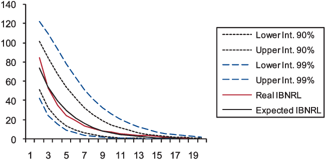
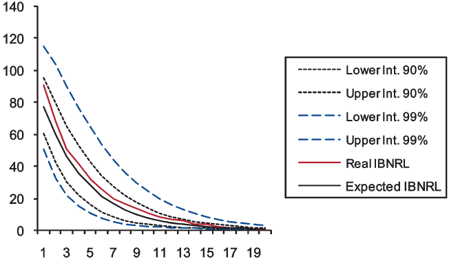
On the basis of the estimation of both the instantaneous claim reporting rate and the volatility of the Wiener process, we check in this subsection the goodness-of-fit by calculating the 90 percent and 99 percent prediction intervals for the IBNRL by means of a normal two-tailed distribution, assuming the catastrophe’s total incurred loss equals 100 (Tables 7, 8, and 9, and Figures 1, 2, and 3).

Figure 1.Prediction intervals for Alcira data series

Figure 2.Prediction intervals for Barcelona data series

Figure 3.Prediction intervals for Valencia data series

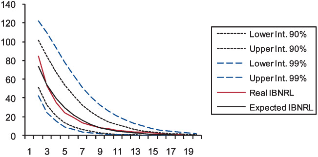
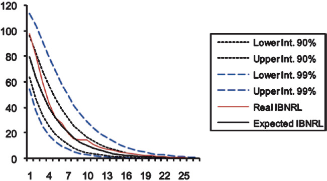
As Figures 1, 2, and 3 show, the prediction intervals are not symmetrical with respect to the expected IBNRL, since data have been exponentially transformed. For either case (namely, 90 and 99 percent intervals), both the real and the expected data remain within the calculated prediction limits. This is a good fit for the IBNRL normal distribution, which demonstrates that our modeling accurately captures the uneven behavior of the claim reporting process over time.

5. Concluding remarks

The continuous model proposed in this paper allows for an easy calculation of catastrophic loss indexes, thus facilitating the pricing of loss index-triggered cat bonds. Unlike previous models [for instance, Cummins and Geman (1995) and Geman and Yor (1997)], we hold the view that the severity of a catastrophe is a random variable resulting from the sum of two other random variables: the IBNRL and the RL.

Previous contributions presuppose a growing RL, which is accordingly represented by means of a geometric Brownian motion. This paper coincides on the first point, but uses the Wiener process to explain the decreasing dynamics of the IBNRL, rather than to describe the evolution of the RL, which is obtained by mere subtraction of the former from the total severity of the specified catastrophe. The loss index is then the RL multiplied by an indicator which varies according to the likelihood of the catastrophic event occurring, thus notably simplifying both the calculation of the index and the estimation of the parameters.

For validation, we have estimated the reporting rate (by maximum likelihood) and the volatility of the model (through calculation of the quasivariance), and concluded that the null hypothesis of the IBNRL log-variations being normally distributed cannot be rejected. To test the goodness-of-fit, finally, we have determined the prediction intervals for both the real and the expected IBNRL, and found that our continuous random model properly describes the behavior of the catastrophic claim reporting process.

Acknowledgments

The author gratefully acknowledges the constructive suggestions and valuable comments from the referees for their significant contribution to improve and clarify this paper. The author also wishes to thank the work of the editors during the review process.