Optimal Layers for Catastrophe Reinsurance

1. Introduction^[1]

Catastrophe reinsurance serves to shield an insurer’s surplus against severe fluctuations arising from large catastrophe losses. By purchasing catastrophe reinsurance, the reinsured trades part of its profit to gain stability in its underwriting and financial results.^[2] If catastrophe risks are independent of other sources of risk and diversifiable in equilibrium, Froot (2001) argued that, under the assumption of a perfect financial market, the reinsurance premium for catastrophe protection should equal the expected reinsurance cost and that a risk-averse insurer would seek the protection against large events over hedging low-retention layers. Gajek and Zagrodny (2004) concluded that if a reinsured has enough money to buy full protection against bankruptcy (ruin), the optimal reinsurance arrangement is the aggregate stop-loss contract with the largest possible deductible.

In practice, financial markets are not perfect, reinsurance prices are significantly higher than those indicated by the theory noted above, and it does not make economic sense for insurers to buy full protection against ruin. Froot (2001) showed that the ratios of the catastrophe reinsurance premium to the expected catastrophe loss can be as high as 20 for certain high-retention layers that have low penetration probabilities.^[3] Facing the reality of relatively high reinsurance prices and the practical economic constraints on the catastrophe reinsurance buyer, primary insurers are reluctant to surrender a large portion of their profit for limited catastrophe reinsurance protections. Thus the reinsured often purchases low reinsurance layers that are subject to a high probability of being penetrated.

Economists have offered many explanations for the inefficiency of the reinsurance market. Borch (1962) investigated the equilibrium of the reinsurance market and found that the reinsurance market will, in general, not reach a Pareto Optimum if each participant seeks to maximize his utility. Froot (2001) identified eight theoretical reasons to explain why insurers buy relatively little reinsurance against large catastrophe events. He found the supply restrictions associated with capital market imperfections (insufficient capital in reinsurance, market power of reinsurers, and inefficient corporate forms for reinsurance) provide the most powerful explanation. As practicing actuaries, the authors believe there are significant limitations on reinsurers’ ability to diversify risk. In the context of catastrophe reinsurance, no reinsurer is big enough to fully diversify away catastrophe risk. To support the risk, a reinsurer needs to hold a prohibitively large amount of additional capital and will, in turn, need to realize an adequate return on such capital.

Froot (2007) found that product-market sensitivity to risk and exposure asymmetry tend to make insurers more conservative in accepting unsystematic risks, more eager to diversify underwriting exposures, and more aggressive in hedging. Even though reinsurance prices are high relative to expected loss, insurers are still willing to seek reinsurance protections.

In this study, the authors do not explore the level of reinsurance price and its reasonableness. We also do not investigate why insurance firms are risk averse to catastrophe losses which are unsystematic and uncorrelated with aggregate market return. Instead, we treat reinsurance price as a predetermined variable in the overall strategic decision-making process and develop an optimal reinsurance strategy for insurers conditioned by their risk appetite, prevailing reinsurance prices at the time a decision is made, and the overall profitability of the enterprise.

This introductory discussion would not be complete if we did not explicitly point out that a reinsurance arrangement, in fact, is a combination of art and science. It often depends on general economic conditions in the state or country of the reinsured and worldwide, the recent history of catastrophe reinsurance in the state or country of the reinsured and worldwide, and the risk characteristics of the reinsured. Both reinsurer and reinsured usually are well informed and are free to negotiate in the spirit of open competition. In the negotiation, it is quite common that certain terms of the treaties would be modified, such as changing the retention level and the size of the layer. In pursuing the optimization process outlined in this paper, we are not attempting to deny or ignore this general art/science characteristic of the reinsurance arrangement. Instead our hope is that knowledge of the optimal balance between profit and risk, as measured using the process outlined in this paper, in the particular circumstances of a reinsured vis-à-vis the then-prevailing market prices, will serve to enhance the quality of the reinsurance decision, ceteris paribus.

Reinsurance arrangements have been studied extensively because of their strategic importance to the financial condition of insurance companies. However, previous studies on optimal catastrophe reinsurance only utilized partial information in the reinsurance decision-making process. Gajek and Zagrodny (2000) and Kaluszka (2001) investigated the optimal reinsurance arrangement by way of minimizing the consequential variance of an insurer’s portfolio. Gajek and Zagrodny (2004) discussed the optimal aggregate stop-loss contract from the perspective of minimizing the probability of ruin. Those studies focus on the risk component, but ignore the profit side of the equation. Bu (2005) developed the optimal reinsurance layer within a mean-variance framework. Insurers are assumed to minimize the sum of the price of reinsurance, the catastrophe loss net of reinsurance recoveries, and the risk penalty. Bu used both the profit and risk components in the optimization. However, his method focused on the catastrophe loss only and ignored the concurrent effect of noncatastrophe underwriting performance on the financial results of the reinsured. In practice, the overall profitability is an important factor impacting the reinsurance strategy because, among other things, it can enhance an insurer’s capability to assume risk.

Lampaert and Walhin (2005) studied the optimal proportional reinsurance that maximizes RORAC (return on risk-adjusted capital). The approach requires the estimation of economic capital based on VaR or TVaR (tail value at risk) at a small predetermined probability. VaR and TVaR are popular in insurance generally and in actuarial circles specifically. VaR is the point at which a “bad” outcome can occur at a predetermined probability, say 1%. TVaR is the mean of all outcomes that are “worse” than the predetermined “bad” outcome. VaR, and especially TVaR, has some convenient features as a risk measure.^[4] TVaR only contemplates severe losses having a probability at or lower than a given probability as the central risk drivers, and it treats those losses linearly. For example, if an insurer has a 5% probability of a loss of $3 million, a 4% probability of a loss of $5 million, a 0.9% probability of a loss of $10 million, and a 0.1% probability of a loss of $100 million, VaR at 1% is $10 million and TVaR is $19 million (10 * 0.9% + 100 * 0.1%)/1%. VaR and TVaR are not consistent with common risk perception from two perspectives: (1) fear is not just of severe losses, it is also of smaller losses (Bodoff 2009). In the case above, $3- and $5-million losses will not contribute to VaR because VaR only considers 1% probability at which risk is generated; (2) risk-bearing entities do not weigh the risk of loss in a linear manner and are more concerned about the incidence of large losses than smaller ones. In other words, risk perception is exponentially, not linearly, increased with the size of loss.

In practice, the RORAC method has been popular in calculating the optimal catastrophe reinsurance layer. In this study, we improve the popular mean-variance approach advocated in academic studies by using lower partial moment (LPM) as the measure of risk, and provide an alternative method for determining optimal reinsurance layers. Compared with the RORAC approach, our method has three advantages. First, it does not involve the calculation of the necessary economic capital, which has no universally accepted definition. Second, by VaR or TVaR, true risk exists only at the tail of the distribution. By LPM, on the other hand, all the losses are considered as generating risk to the risk-bearer, but severe losses contribute to LPM disproportionately. Third, the estimation of variance and semivariance is relatively robust compared to VaR and TVaR in the context of catastrophe losses. The tail estimation of remote catastrophe losses generally is not robust, and is very sensitive to the assumptions about the underlying distribution, especially at high significance levels. The limitations of the proposed method are the limitations inherent to the mean-variance framework. It can be difficult to estimate the risk-penalty coefficient, as the parameter is often time-dependent and subject to management’s specific risk appetite.

This paper improves the previous mean-variance optimal reinsurance studies from two perspectives. First, it considers noncatastrophe and catastrophe losses simultaneously. Second, the risk is measured by LPM (semivariance), which is a more reasonable and appropriate risk measure than the traditional risk measures, such as total variance, used in previous studies (i.e., Borch 1982; Lane 2000; Kaluszka 2001; Bu 2005). Even though the authors investigate the optimal layers in the context of catastrophe reinsurance, the proposed method can be easily applied to aggregate excess-of-loss (XOL) treaties and occurrence XOL treaties that cover shock losses at individual occurrence/claim levels.

2. Risk-adjusted profit model

Insurance companies buy catastrophe reinsurance to reduce potential volatility in earnings and to provide balance sheet protection from catastrophic events. However, reinsurance comes at a cost, and therefore attaining an optimal balance between profit levels after the effect of catastrophe reinsurance and the reduction in their risk exposure is important. Buying unnecessary or “excessive” reinsurance coverage would give up more of the reinsured’s underwriting profit than is necessary or desirable. Buying inadequate reinsurance coverage would still expose the reinsured to the volatility engendered by the risk of large catastrophe events, the reinsurance cover notwithstanding. The value of reinsurance is the stability gained or the risk reduced and the cost is the premium paid less the loss recovered. As Venter (2001) pointed out, the analysis of a reinsurance arrangement is the process of quantifying this cost/benefit relationship. It is self-evident that in an insurance company’s decision-making process, a relatively certain, but maximal, profit is preferable over other, perhaps higher profit potentials that are also exposed to the risk of large catastrophic losses. Following the classic meanvariance framework in financial economics, a reinsured will buy reinsurance to maximize its risk-adjusted profit, defined as^[5]

$$\mathrm{RAP}=E(r)-\theta * \operatorname{Var}(r) \tag{1}$$

where r is the net underwriting profit rate, E(r) is the mean of r and Var(r) is its variance. θ * Var(r) is the penalty on risk. θ is the risk-penalty coefficient: the higher the risk-penalty θ, the greater is the reinsured’s risk aversion. If θ = 0, the reinsured is risk-neutral. It will try to maximize profit and not care about risk. In this scenario, it will not give up any profit to purchase reinsurance.

The most common measurement of risk is the variance associated with a particular outcome. Variance reflects the magnitude of uncertainty (variability) in underwriting results, and how widely spread the values of the profit rate are likely to be around the mean. Therefore, within a variance framework, all the variations, both desirable and undesirable, are viewed as manifestations of risk. Large favorable swings will lead to a large variance, but insurers certainly have no problem with such favorable underwriting results. Markowitz (1959) pointed out the drawbacks of using total variance as a measure of risk, as there is implicitly and directly a cost to both upside and downside movements.

Fishburn (1977) argued that risk should be measured in terms of only below-target returns. Hogan and Warren (1974) and Bawa and Lindenberg (1977) suggested using LPM to replace total variance as the risk measure:

$$\operatorname{LPM}(T, k)=\int_{-\infty}^{T}(T-r)^{k} d F(r) \tag{2}$$

where T is the minimum acceptable profit rate, k is the moment parameter which measures one’s risk perception sensitivity to large loss, and F(r) is the probability function of r. Unlike total variance, LPM only measures the unfavorable variation (e.g., when r < T) as risk. Because LPM does not change with favorable deviations, it would seem to be a superior measure of risk.

When T is triggered at the 1% probability level and k = 1, LPM is equal to 0.01 * TVaR. When the distribution is symmetric, T is the mean, and k = 2, it is equal to 0.5 * variance. LPM combines the advantages of variance and TVaR. It is superior to variance by not treating the favorable outcomes as risks. It is superior to TVaR because (1) it considers small and medium losses as risk components, and (2) it provides nonlinear increasing penalties on larger losses when k > 1. In the example above, suppose a $100 million loss will cause a financial rating downgrade, while a $10 million loss merely causes a bad quarter. Management inevitably will perceive a $100 million loss to be more than 10 times as bad as a $10 million loss. By VaR, a $100 million loss is 10 times as bad as a $10 million loss. By LPM with k = 1.5, the risk of a $100 million loss is 31.6 times that of a $10 million loss; and by LPM with k = 2, it is 100 times. The k value is a direct measure of risk aversion to large losses.

When k = 2, LPM is often called “semivariance” (it excludes the effects of variance associated with desirable outcomes in the measurement of risk) and has been gaining greater acceptance. By formula, semivariance is defined as

$$\operatorname{SV}(T)=\int_{-\infty}^{T}(T-r)^{2} d F(r). \tag{3}$$

A growing number of researchers and practitioners are applying semivariance in various financial applications. For example, Price, Price, and Nantell (1982) showed that semivariance helps to explain the puzzle of Black, Jensen, and Scholes (1972) and Fama and MacBeth (1973) that low-beta stocks appear systematically underpriced and high-beta stocks appear systematically overpriced. However, to date, the casualty actuarial literature has seldom used the semivariance as a risk management tool and neither does it appear much in practice.^[6]

Generally, a decision-maker can be expected to be more concerned with the semivariance than with the total variance. Using downside risk instead of total variance, the downside-risk-adjusted profit (DRAP) becomes

$$\operatorname{DRAP}=\operatorname{Mean}(r)-\theta * \operatorname{LPM}(T, k), \tag{4}$$

where θ is the penalty coefficient on downside risk.

Three parameters T, k, θ in the DRAP formula interactively reflect risk perception and risk aversion. With these three parameters, the DRAP method provides a comprehensive and flexible capacity to capture risk tolerance and appetite.

T is the benchmark point of profit below which the performance would be considered as “downside” (lower than is minimally unacceptable). T can be a target profit rate, the risk-free rate, zero, or even negative, depending on one’s risk perception. When T is at the very right tail of r, only large losses contribute to the downside risk. T can vary by the mix of lines of business. For example, for long tail lines, negative underwriting profits may be tolerable because of anticipated investment income on loss reserves.

The moment parameter k reflects one’s risk perception as the size of loss grows: k > 1 implies exponentially increasing loss perception to large losses; 0 < k < 1 represents concavely increasing loss perception to large losses; k =1 implies linearly increasing loss perception. In general, k is larger than 1 since fear of extreme events that can lead to a financial downgrade is greater than the fear of multiple smaller losses. Because semivariance is the most popular LPM, we choose k = 2 to illustrate our approach in the case study presented below.

The risk aversion level is represented by θ, which is a function of T and varies according to its values. For example, when T = 0, all the underwriting losses contribute to LPM(0, k); when T = −10%, only losses exceeding the 10% loss rate contribute to LPM(−0.1, k). LPM(−0.1, k) represents a much more severe risk than LPM(0, k). θ is also a function of k. For example, LPM(T, 1) and LPM(T, 2) are at different scales because the former is at the first moment and the latter is at the second moment. θ should vary with k because k changes the scale of risk measure.

Note that θ may not be constant across loss layers. For example, when k = 1, LPM is a linear function of loss. For a run of smaller losses that cause a “bad” quarter, θ may be very small. For losses that cause a “bad” year or eliminate management’s annual bonus, θ may be larger. For losses that lead to a financial downgrade or the replacement of management, θ will be even larger. Interested readers can expand the models in this paper by adding a series of risk-penalties upon predetermined loss layers with various risk aversion coefficients. When k ≥ 2, because LPM increases exponentially with extreme losses, it may not be necessary to impose higher risk-penalty coefficients on higher layers.

In addition, k may not be constant across loss layers. The scale of loss impacts the value of k. If k is constant, say k = 2, it implies that $100 million loss is 100 times worse than $10 million loss. It also indicates that $100 loss is 100 times worse of $10 loss. The latter, in general, is not true because of linear risk perception when viewing a smaller nonmaterial loss. In the context of reinsurance, k might be closer to one at a working layer (low retention with high probability of penetration) and would increase for higher excess layers. Interested readers can expand the models in this paper by adding a series of risk-penalties upon predetermined loss layers with various moment parameters.

The academic tradition in financial economics has been to set θ as a constant and k = 2.^[7] Assuming an individual has a negative exponential utility function u(r)= −exp(−A * r), where A > 0. If r is normally distributed, the expected utility is E[u(r)] = −exp[−A * E(r) + 0.5A² * Var(r)]. Maximizing E[u(r)] is equivalent to maximizing E(r) − 0.5A * Var(r). Also, −u′′(r)/u′(r), which is equal to A in this specific case, is often referred as the “Arrow-Pratt measure of absolute risk aversion.” Constant θ and k = 2 are built-in features under the assumptions of negative exponential utility function and normality. Alternatively, interested readers can use negative exponential utility, logarithmic utility, or define their own concavely increasing utility curves, and select the optimal reinsurance layer to maximize the expected utility function.^[8] To simplify the illustration and to be consistent with academic tradition, we use a constant θ and k = 2 in the case study.

An inherent difficulty in mean-variance type of analysis is the need to estimate the risk-penalty coefficient empirically. The key is to measure how much risk premium one is willing to pay for hedging risk. The flip counter-party question is how much investors would require for assuming that risk. For overall market risk premium, one can obtain the market risk premium by subtracting the risk-free treasury rate from market index return. For example, if the market return is 10%^[9] and the risk-free rate is 5.5%, the risk premium is 4.5%, or 45% of total “profit.” For the risk premium in the insurance/reinsurance market, one can use the market index for insurance/reinsurance companies. For the risk premium in catastrophe reinsurance, one can compare catastrophe bond rates to the risk-free rate. For example, if the catastrophe bond yield is 12%,^[10] the treasury rate yield is 5.5%, and the expected loss from default is 0.5%, then the risk premium^[11] is 6%, consisting of 50% of total yield.

The methods above provide objective estimation of θ assuming that management’s risk appetite is consistent with the market. In reality, θ varies by risk-bearing entity. Each risk-bearing entity has its own risk perception and tolerance. To measure management’s risk aversion, one can obtain θ by asking senior executives, “In order to reduce downside risks, how much of the otherwise available underwriting profit per unit of risk are you willing to pay?” The answer to a single question may not be sufficient to pin down the value of theta. Most likely management would require information about expected results under optimal reinsurance programs at various values of theta to fully understand the implications of the final theta value selected. To replicate the sensitivity tests that management may perform when determining the utility function, the case study provides optimal insurance solutions at various values of theta.

For the same management within the same institution, θ often is time-variant^[12] as the risk appetite often changes to reflect macro economic conditions or micro financial conditions. For example, after a financial crisis, insurance companies may become more risk averse. θ also varies by the mix of business. For lines with little catastrophe potential, such as personal auto, the tolerance on downside risk might be higher and θ would be smaller. For lines with higher catastrophe potential, such as homeowners, θ can be larger. θ is difficult to estimate because of its subjective nature. Actuarial judgment plays an important role when determining the risk-penalty coefficient.

In the context of catastrophe reinsurance, the layers are bands of protection associated with catastrophe-triggered loss amounts. Outside of price, the main parameters of a catastrophe layer are the retention, the coverage limit, and the cession percentage within the layer of protection. Retention is the amount that the total loss from a catastrophe event must exceed before reinsurance coverage attaches. The limit is the size of the band above the retention that is protected by reinsurance. The cession percentage is the percentage of the catastrophe loss within the reinsurance layer that will be covered by the reinsurer. The limit multiplied by the cession percentage is the maximum reinsurance recovery from a catastrophe event within that particular band of loss. The coverage period of catastrophe reinsurance contracts is typically one year. Let x_i denote the gross incurred loss from the $i^{th}$ catastrophe event within a year, and Y be the total gross noncatastrophe loss of the year. Let R be the retention level of the reinsurance, L be the coverage layer of the reinsurance immediately above R,^[13] and ϕ be the coverage percentage within the layer.

The loss recovery from reinsurance for the ith catastrophe event is

$$G\left(x_{i}, R, L\right)=\left\{\begin{array}{cl} 0 & \text { if } \quad x_{i} \leq R \\ \left(x_{i}-R\right) * \phi & \text { if } \quad R<x_{i} \leq R+L . \\ L * \phi & \text { if } \quad x_{i}>R+L \end{array}\right. \tag{5}$$

Let EP be the gross earned premium, EXP be the expense of the reinsured, N be the total number of catastrophe events in the reinsurance contract year, RP(R,L) be the reinsurance premium, which is a decreasing function of R and an increasing function of L, and RI be the reinstatement premium.

The underwriting profit gross of reinsurance is

$$\pi=\mathrm{EP}-\mathrm{EXP}-Y-\sum_{i=1}^{N} x_{i} .\tag{6}$$

Reinstatement premium is a pro rata reinsurance premium charged for the reinstatement of the amount of reinsurance coverage that was “consumed” as the result of a reinsurance loss payment under a catastrophe cover. The standard practice is one or two reinstatements. The number of reinstatements imposes an aggregate limit on catastrophe reinsurance. The reinstatement premium after the ith catastrophe event is

$$\mathrm{RI}\left(x_{i}, R, L\right)=\mathrm{RP}(R, L) * G\left(x_{i}, R, L\right) / L .\tag{7}$$

The underwriting profit net of reinsurance is

$$\begin{aligned} \pi= & \mathrm{EP}-\mathrm{EXP}-Y-\sum_{i=1}^{N} x_{i}-\mathrm{RP}(R, L) \\ & +\sum_{i=1}^{N} G\left(x_{i}, R, L\right)-\sum_{i=1}^{N} \mathrm{RI}\left(x_{i}, R, L\right). \end{aligned} \tag{8}$$

The underwriting profit rate net of reinsurance is

$$\begin{aligned} r= & 1-\frac{\mathrm{EXP}+Y+\mathrm{RP}(R, L)}{\mathrm{EP}} \\ & -\frac{\sum_{i=1}^{N} x_{i}-G\left(x_{i}, R, L\right)+\mathrm{RI}\left(x_{i}, R, L\right)}{\mathrm{EP}} . \end{aligned} \tag{9}$$

Thus the optimal layer is that combination of R and L which maximizes DRAP:^[14]

$$\operatorname{Max}_{R, L} \operatorname{Mean}(r)-\theta * \mathrm{SV}(r), \quad \text { subject to C.} \tag{10}$$

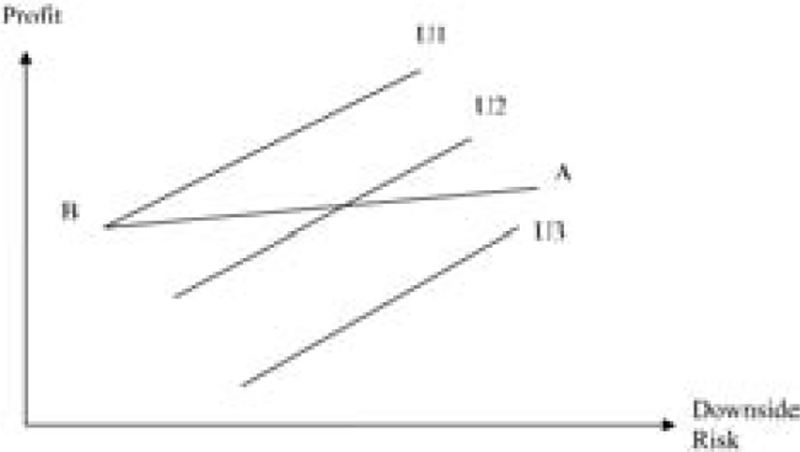
Capital asset pricing model suggests that firms in a perfect market are risk neutral to unsystematic risks. If reinsurers are adequately diversified and price as though they are risk neutral, the reinsurance premium would be equal to the expected reinsurance cost.^[15] That is, the total premium paid by reinsured, $\mathrm{RP}(R, L)+\sum_{i=1}^N \mathrm{RI}\left(x_i, R, L\right)$, is equal to the expected reinsurer’s loss cost, $\sum_{i=1}^N G\left(x_i, R, L\right)$ plus reinsurer’s expense. In this case, reinsurance will significantly reduce the volatility of the underlying results of the insured over time, but slightly reduce the expected profit by the reinsurance expense over the same period of time. Figure 1 shows reinsurance optimization under the assumption of perfect market diversification. A is the combination of profit and downside risk without any reinsurance. B is the profit and risk with full reinsurance. B is not downside-risk-free because noncatastrophe loss could cause the profit to fall below the minimum acceptable level. Line AB is the efficient frontier with all possible reinsurance layers. Closer to B, it represents buying a great deal of reinsurance coverage. Closer to A, it represents buying minimal reinsurance coverage. Under the assumption, the reinsurance premium only covers reinsurer’s costs, and the line is relatively flat.^[16] U1, U2, and U3 are the utility curves. The slope of those lines is the risk-penalty coefficient θ. The steeper the curve, the more risk-averse. All the points on a given curve provide the exact same utility. The higher utility curve represents the higher utility. The utilities on line U1 are higher than those on lines U2 and U3. An insurance company gains the highest utility at point B. Thus maximizing the risk-adjusted profit is equivalent to minimizing the downside risk. The optimal solution occurs when R = 0 and L = + ∞. A retention equal to zero coupled with an unlimited reinsurance layer will completely remove the volatility from catastrophe events with a low cost (reinsurance premium-recovery). Under the perfect market diversification assumption, the proposed method yields a solution consistent with Froot (2001).

Figure 1.Reinsurance optimization under the assumption of perfect diversification

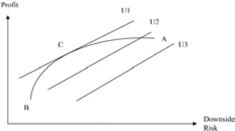
In practice, however, because of the need to reward reinsurers for taking risk, the reinsurance price RP(R,L) is always larger than the expected reinsurer’s loss cost. The expected loss/premium ratio is generally a decreasing function of retention R. The higher the retention R, the lower the expected reinsurance loss ratio. From the relationship between risk transfer and reinsurance premium, a higher layer implies a higher level of risk being transferred to the reinsurer. To support the risk associated with higher layers, the reinsurer needs more capital and thus requires a higher underwriting margin. Therefore, a reinsured has to pay a larger risk premium on higher layers to hedge its catastrophe risk. In practice, $E\left(\sum_{i=1}^N G\left(x_i, R, L\right)\right) / \mathrm{RP}(R, L)$ is often less than 40%, and even below 10% for high retention treaties. The relatively high prices associated with high retentions often deter the reinsured from purchasing coverage at those levels. Subject to the constraints imposed by reinsurance prices and the willingness of the reinsured to pay, as Froot (2001) discussed, the optimal solutions are often low reinsurance retentions at a relatively low price and a high probability of being penetrated. Figure 2 shows reinsurance optimization in reality. As in Figure 1, curve AB represents the efficient frontier. Because reinsurance companies cannot fully diversify catastrophe risk and require higher returns to assume the risk on higher layers, AB is a concave curve: from A to B, the slope becomes steeper to reflect higher risk premiums associated with higher layers. Close to point B, the slope is very steep to reflect the extra capital surcharge at the top layers. Of all the possible reinsurance layers, point C provides the highest utility (or DRAP) to the reinsured.

Figure 2.Reinsurance optimization in reality

3. A case study

3.1. Key parameters

Suppose an insurance company with $10 billion^[17] gross earned premium plans to purchase catastrophe reinsurance. Within one year, the number of covered catastrophe events is normally distributed^[18] with a mean of 39.731 and a standard deviation of 4.450; and the gross loss from a single catastrophe event is assumed to be lognormally distributed. The logarithm of the catastrophe loss has a mean of 14.478 and a standard deviation of 1.812,^[19] which imply a mean of $10.02 million and a standard deviation of $50.77 million for the catastrophe loss from one event. The mean of the aggregate gross loss from all the catastrophe events within a year is $397.94 million and the standard deviation is $322.92 million. The expense ratio of the insurance company is assumed to be 33.0%. The aggregate gross noncatastrophe loss is also assumed to be lognormally distributed with a logarithm of noncatastrophe loss mean of 22.497 and standard deviation of 0.068. This implies that the mean of gross noncatastrophe loss is $5.91 billion and the standard deviation is $402.10 million. Assuming catastrophe and noncatastrophe losses are independent,^[20] the mean of the aggregate gross loss is $6.30 billion and the standard deviation is $515.72 million. The mean underwriting profit rate is 3.93% and the standard deviation is 5.16%. The numerical study is based on this hypothetical company using the simulated noncatastrophe and catastrophe loss data. The simulation is repeated 10,000 times. In each simulation, the noncatastrophe loss and catastrophe losses within a year are generated, the losses covered by the reinsurance treaty are calculated by Equation (5), and the total profit rate is calculated by Equation (9) assuming two reinstatements. Let r_m be the profit rate from the mth round of simulation. The semivariance is

$$\mathrm{SV}(R, L)=\frac{1}{10000} \sum_{m=1}^{10000}\left(\min \left(r_{m}-T, \quad 0\right)\right)^{2}. \tag{11}$$

Equation (11) is a discrete formula of semivariance, which is an approximation of Equation (3).

Let us assume that reinsurance will cover 95% of the layer (R,L) and UL is the upper limit of the covered reinsurance layer (R,L), UL = R + L. For reinsurance prices, we fit a nonlinear curve using actual reinsurance price quotes.^[21] The fitted reinsurance price of layer (R,L) is^[22]

$$\begin{aligned} \mathrm{RP}(R, L)= & 1.2300 *(\mathrm{UL}-R)+1.2978 * 10^{-4} \\ & *\left(\mathrm{UL}^{2}-R^{2}\right)-1.3077 * 10^{-8} \\ & *\left(\mathrm{UL}^{3}-R^{3}\right)-0.1835 \\ & *(\mathrm{UL} * \log (\mathrm{UL})-R * \log (R)) \\ & +45.4067 *(\log (\mathrm{UL})-\log (R)) . \end{aligned}$$

The appendix contains both the quoted reinsurance prices and the fitted reinsurance prices. The actual prices below layer ($1,800 million, $3,050 million) are derived by combining the six layers with known quotes. Simon (1972) and Khury (1973) discussed the importance of maintaining the logical consistency among various alternatives, especially on pricing. The fitted price curve is logically consistent in two ways: (1) the rate-on-line is strictly decreasing with retention and consistent with actual observations; (2) for two adjacent layers, the sum of prices is equal to the price of the combined layer, that is, RP(R,L₁ + L₂) = RP(R,L₁) + RP(R + L₁, L₂).

The minimum acceptable profit rate T and risk-penalty coefficient θ vary by business mix and by risk-bearing entity. In this case study, 0% is selected as the minimum acceptable profit rate for illustrative purposes. So, only underwriting losses contribute to the risk calculation. For θ, we use three values, 16.71, 22.28, and 27.85. Those coefficients represent management’s willingness to pay 30%,^[23] 40%, and 50% of underwriting profits to hedge downside risk, respectively. The risk-penalty coefficients in the case study are selected solely for illustrative purposes.

3.2. Numerical results

In the simulation, we generate catastrophe loss and noncatastrophe loss for 10,000 years. In the instant case, 397,257 catastrophe events are generated. Table 1 summarizes the losses covered by reinsurance for quoted layers; Table 2 reports the distribution summary of underwriting profit rates net of reinsurance and the risk-adjusted profit rates for quoted layers and their continuous combinations.

As illustrated in Table 1, a catastrophe loss has a 10.18% chance to penetrate the retention level of $305 million within one year. So, roughly in one of 10 years, the reinsured will obtain recoveries by purchasing the reinsurance for this layer. The higher the retention level, the lower the probability that the catastrophe loss penetrates the layer. For example, the catastrophe loss has only a 0.40% chance of penetrating a retention level of $1,800 million.^[24] This is expected because the frequency of a very large catastrophe loss is relatively small. For the layer ($305 million, $420 million), the reinsurance price is $20.8 million, while the mean of loss recovered from the reinsurance is $8.9 million. The ratio of reinsurance recovery to reinsurance premium is 42.59%. The reinsurance is costly, especially for the higher layers. For the top layer ($1,800 million, $3,050 million), the reinsurance price is $39.1 million while the mean of loss recovered by reinsurance is $2.6 million. The ratio of recovery to premium is 6.58%. So, the capital charge on the top layer of reinsurance tower is very high.

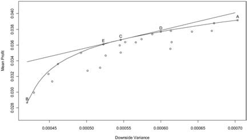
Table 2 reports the probability of net underwriting loss, the probability of severe loss (defined as more than 15% of net underwriting loss), mean of profit, variance of profit, semivariance of profit, and risk-adjusted profits at θ = 22.28. The scattered dots (except for A, C, D, and E) in Figure 3 represent the quoted reinsurance layers and all possible continuous combinations of those layers. A represents the no reinsurance scenario and B represents the maximal reinsurance scenario of stacking all quoted layers. The slope from A to B becomes steeper and reflects the reality of reinsurance pricing. The concave curve in Figure 3 represents the efficient frontier. Not unexpectedly, some of the quoted reinsurance layers are not at the frontier: one can find another layer to produce a higher return at the same downside risk or a lower risk at the same return. For example, layer ($305 million, $1,030 million) is not efficient with a mean profit and a semivariance of 3.465% and 0.053%, respectively. Layer ($610 million, $1,800 million) is clearly superior because it increases average return (3.500%) while reducing risk (0.049%).

Figure 3.Reinsurance efficient frontier

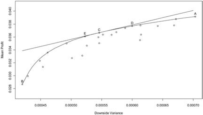
As shown in Table 2, the reinsured will maximize its DRAP by selecting the layer ($680 million, $1,390 million) assuming a 22.28 risk-penalty coefficient, which implies that the management would be willing to pay 1.567% of gross premium (40% of gross underwriting profit) to hedge downside risk. For a lower layer, even though the layer has a greater chance to be penetrated, the potential risk of catastrophe loss is tolerable by the reinsured. For a higher layer, the reinsurance price is too high compared to the risk mitigation it provides. Point C in Figure 3 represents this optimization option. The straight tangent line represents the utility curve at θ = 22.28. All other possible layers are below the line and therefore have lower utility values.

It is also clear from Table 2 that catastrophe reinsurance does not increase the probability of being profitable in the instant case. Without reinsurance, the probability of underwriting loss is 18.41%. With reinsurance of various layers, the probabilities of underwriting loss are over 19%. The purpose of reinsurance is to buy protections against large events. Without reinsurance, the chance of severe loss is 0.48%, or roughly one in 200 years. With a minimal reinsurance layer ($305 million, 420 million), it reduces to 0.42%, or roughly one in 250 years. With the optimal reinsurance layer ($680 million, $1,390 million), the chance of severe loss reduces to 0.21%, or roughly one in 500 years.

If the reinsured is less risk-averse, the optimal layer will be narrower and the retention level will be higher. As shown in Table 3, when θ = 16.71, or when the management would like to pay 1.175% of gross premium (30% of total underwriting profit) to hedge its downside risk, the optimal layer is ($795 million, $1,220 million). On the contrary, if the reinsured is more risk-averse, the optimal layer will be wider and the retention level will be lower. For example, when θ = 27.85, or the management would like to pay 1.958% of gross premium (50% of total underwriting profit) to hedge its downside risk, the optimal layer is ($615 million, $1,460 million). Point D in Figure 3 represents the optimization at reduced risk aversion while Point E represents the optimization at higher risk aversion.

In practice, actuaries may not be able to choose reinsurance layers from an unlimited pool of options. They often need to select a layer or a combination of layers from a limited number of options. A simple method is to calculate the riskadjusted profit for the candidate layers using Equation (9) and select a layer associated with the highest score. Layer ($610 million, $1,030 million) is the best of the six quoted options. In this case, actuaries do not need to fit a nonlinear curve on reinsurance prices and to solve the complicated optimization problem.

The underwriting performance may impact the reinsurance selection from two perspectives: (1) the more profitable the business, the more risk the insurer can retain, and the less reinsurance the insurer may be willing to buy; (2) the more profitable the business, the more capital can be deployed for reinsurance, and the more reinsurance the insurer is able to buy. The optimal reinsurance layer, assuming a 3.93% gross underwriting profit rate with θ = 22.28, is ($680 million, $1,390 million). If the company could make 2% more underwriting profit by lowering its noncatastrophe loss ratio, the reinsurance optimizations could be formularized by the following parameters:^[25]

1. The benchmark point for minimum acceptable profit may increase to 2%. In this case, the semivariance will not be impacted by a profitability change; the optimal layer remains the same as ($680 million, $1,390 million).

2. The minimum acceptable profit rate remains at 0%. In this case, the semivariance reduces with improved profitability. The semivariance decreases from 0.07% to 0.05% and downside deviation from 2.652% to 2.240%. This is because smaller catastrophe events no longer produce underwriting losses, and larger events would produce 2% less loss.

   a. If the penalty on the semivariance remains at 22.28, the optimal layer becomes ($740 million, $1,420 million). The insurer would maximize its risk-adjusted profit by retaining more loss from relatively small events (higher retention). This is because the reinsured has more underwriting profit to cover smaller catastrophe events. And by increasing the retention level, it could have additional capital to buy more protection from a higher layer ($1,390 million, $1,420 million). The limit is reduced from $710 million to $680 million because the downside risk is smaller.

   b. If the reinsured would like to use the same level of profit, or 1.567% of gross premium, to fully hedge downside risk, θ would be 31.22. In this scenario, the optimal layer is ($630 million, $1,555 million). The reinsured would like to buy a wider layer with a lower retention due to increased risk-aversion (willing to pay the same amount of price to hedge a semivariance that is 28.6% smaller than before).

4. Conclusions

When selecting reinsurance layers for catastrophe loss, the reinsured weighs two dimensions in the decision making process: profit and risk. The reinsured would give up too much of its underwriting profit if purchasing excessive reinsurance. On the other hand, the reinsured would still be under the risk of large catastrophe losses if carrying little reinsurance. This study explores the determination of the optimal reinsurance layer for catastrophe loss. The reinsured is assumed to be risk-averse and chooses the reinsurance layer that maximizes the underwriting profit net of reinsurance adjusted for downside risk. It provides a theoretical and practical model under classical mean-variance framework to estimate the optimal reinsurance layer. Theoretically, the paper improves previous studies by utilizing both catastrophe and noncatastrophe loss information simultaneously and using the lower partial moment to measure risk. Practically, the optimal layer is determined numerically by the risk appetite of the reinsured, the reinsurance price quotes by layer, and the loss (frequency and severity) distributions of the business written by the reinsured. The proposed approach uses three parameters to reflect the insurer’s risk perception and risk aversion. T is the minimum acceptable profit and the benchmark point to define “downside.” The moment that represents one’s risk perception of larger losses is k; the higher the k, the greater the fear of severe losses. θ is the risk-penalty coefficient which represents one’s risk aversion. The higher the θ, the greater the risk aversion to downside risks. The DRAP (downside-risk-adjusted profit) framework provides a flexible approach to capture the insurer’s risk appetite comprehensively and precisely. All the information required by the model should be readily available from catastrophe modeling vendors and the actuarial database of an insurance company.

Additionally, we would like to make the following concluding remarks:

1. From the perspective of enterprise risk management (ERM), catastrophe insurance is a risk management tool to mitigate one of many risks faced by insurance companies. Catastrophe reinsurance should not be arranged or evaluated solely upon the information of catastrophe losses. Instead, its arrangement should be viewed concurrently with other types of risks, such as noncatastrophe underwriting risk and various investment risks. In this paper we consider both catastrophe and noncatastrophe losses and the analysis (simulation) is carried out with both sets of variables operating concurrently. This particular path views the catastrophe reinsurance cover as a part of the ERM process. We believe the decision reached by viewing the transaction as a step in the ERM process to be a superior decision. This idea may be extended to all other elements of reinsurance considered and/or utilized by an insurer. In effect, our suggestion is that the reinsurance decision, for catastrophe reinsurance and otherwise, is an important element of the total ERM process.

2. The reinsurance purchase decision is seldom, if ever, guided solely by the dry mechanics of pricing a layer above a particular attachment point to pay a certain percentage of the covered layer. An aspect of the transaction that goes beyond the mechanical factors deals with “who” the prospective reinsurer is. This is an important input item, but it is always an intangible. The size of the reinsurer, the size of its surplus, the financial rating of the reinsurer, the length and quality of the relationship with the reinsurer, how much of the reinsurance is retained for its own account, and so forth form important intangibles that are impossible to factor into any simulation. All the same, these factors do operate and they can influence the final decision.

3. Another aspect of the reinsurance decision is the way the ultimate decision maker may be able to use the outputs of modeling such as those proposed in this paper. The models and their output in effect provide the ultimate decision maker with some absolute points of reference that can be factored into the final decision. For example, if the model results show a clearly economically advantageous reinsurance proposition is being offered, the ultimate decision maker now has some “elbow room” to fully capitalize on the advantage that is being offered: he may seek to expand layers of coverage, extend the terms of coverage, add additional reinstatement provisions, and so on. On the other hand, if the proposed reinsurance is particularly disadvantageous, the ultimate decision maker also is well armed to seek alternatives that are consistent with his appetite for risk: change the point of attachment, change the size of the reinsured layer, seek outside bids for the same coverage, and so on. In all cases, the knowledge that is imparted from these simulations to the ultimate decision maker enhances his level of comfort with what is being offered as well as with any final decision.

4. The downside risk measure and utility function (downside-risk-adjusted profit) in this study can be adapted to analyze whether an insurance company should write catastrophe exposures and the design of the catastrophe reinsurance program would be one component of such an analysis. For example, if the profit in a property line is not high enough to cover reasonable reinsurance costs, or even negative, it is better to not write that property line. The risk-adjusted profit of the primary insurer without the property line will be higher than that by adding the line and buying the optimal catastrophe reinsurance cover. In reality, a property line may not be profitable and it may not be a viable option to completely exit or even shrink the line. Under the scenario of unprofitable property lines with predetermined exposures, the proposed method can still help the primary insurer to find an optimal reinsurance solution and to mitigate severe downside pains from property lines by giving up a portion of profit from other profitable lines.

5. Uncertainty in modeling and estimating net underwriting profit is an important consideration. Model and parameter risks inherent in catastrophe loss simulations can influence actual vs. perceived costs as well as the optimal amount of capacity companies choose to buy.

Finally, there is no question that, when all is said and done, the ultimate decision maker has to weigh many things, both objective and subjective, on the way to finalizing the reinsurance decision. Having the results of the simulations presented in this paper serves to improve the quality of decision making.