


1. Introduction
Over the years, there have been a number of stochastic loss reserving models that provide the means to statistically estimate confidence intervals for loss reserves. In discussing these models with other actuaries, I find that many feel that the confidence intervals estimated by these methods are too wide. The reason most give for this opinion is that experienced actuaries have access to information that is not captured by the particular formulas they use. These sources of information can include intimate knowledge of claims at hand. A second source of information that many actuarial consultants have is the experience gained by setting loss reserves for other insurers.
As one digs into the technical details of the stochastic loss reserving models, one finds many assumptions that are debatable. For example, Mack (1993), Barnett and Zehnwirth (2000), and Clark (2003) all make a number of simplifying assumptions on the distribution of an observed loss about its expected value. Now it is the essence of predictive modeling to make simplifying assumptions. Which set of simplifying assumptions should we use? Arguments based on the “reasonability” of the assumptions can (at least in my experience) only go so far. One should also test the validity of these assumptions by comparing the predictions of such a model with observations that were not used in fitting the model.
Given the inherent volatility of loss reserve estimates, testing a single estimate is unlikely to be conclusive. How conclusive is the following statement?
Yes, the prediction falls somewhere within a wide range.
A more comprehensive test of a loss reserve model would involve testing its predictions on many insurers.
The purpose of this paper is to address at least some of the issues raised above.
-
The methodologies developed in this paper will be applied to the Schedule P data submitted on the 1995 NAIC Annual Statement for each of 250 insurers.
-
The stochastic loss model underlying the methods of this paper will be the collective risk model. This model combines the underlying frequency and severity distributions to get the distribution of aggregate losses. This approach to stochastic loss reserving is not entirely new. Hayne (2003) uses the collective risk model to develop confidence regions for the loss reserve, but the regions assume that the expected value of the loss reserve is known. This paper makes explicit use of the collective risk model to first derive the expected value of the loss reserve.
-
Next, this paper will illustrate how to use Bayes’ Theorem to estimate the predictive distribution of future paid losses for an individual insurer. The prior distributions used in this method will be “derived” by an analysis of loss triangles for other insurers. This method will provide some of the “experience gained by setting loss reserves for other insurers” that is missing from existing statistical models for calculating loss reserves. An advantage of such an approach is that all assumptions (i.e., prior distributions) and data will be clearly specified.
-
Next, this paper will test the predictions of the Bayesian methodology on data from the corresponding Schedule P data in the corresponding 2001 NAIC Annual Statements. The essence of the test is to use the predictive distribution derived from the 1995 data to estimate the predicted percentile of losses posted in the 2001 Annual Statement for each insurer. While the circumstances of each individual insurer may be different, the predicted percentiles of the observed losses should be uniformly distributed. This will be tested by standard statistical methods.
-
Finally, this paper will analyze the reported reserves and their subsequent development in terms of the predictive distributions calculated by this Bayesian methodology.
The main body of the paper is written to address a general actuarial audience. My intention is to make it clear what I am doing in the main body. In the Appendix, I will discuss additional details needed to implement the methods described in some of the sections.
2. Exploratory data analysis
The basic data used in this analysis was the earned premium and the incremental paid losses for accident years 1986 to 1995. The incremental paid losses were those reported as paid in each calendar year through 1995.
The data used in this analysis was taken from Schedule P of the 1995 NAIC Annual Statement, as compiled by the A. M. Best Company. I chose the Commercial Auto line of business because the payout period was long enough to be interesting but short enough so that ignoring the tail did not present a significant problem. The estimation of the tail is beyond the scope of this paper.
I selected 250 individual insurance groups from the hundreds that were reported by A. M. Best. Criteria for selection included: (1) at least some exposure in each of the years 1986 to 1995; (2) no abrupt changes in the exposure from year to year; and (3) no sharp decreases in the cumulative payment pattern. There were occasions when the incremental paid losses were negative, but small in comparison with the total loss. In this case, I treated the incremental losses as if they were zero. I believe this had minimal effect on the total loss reserve.
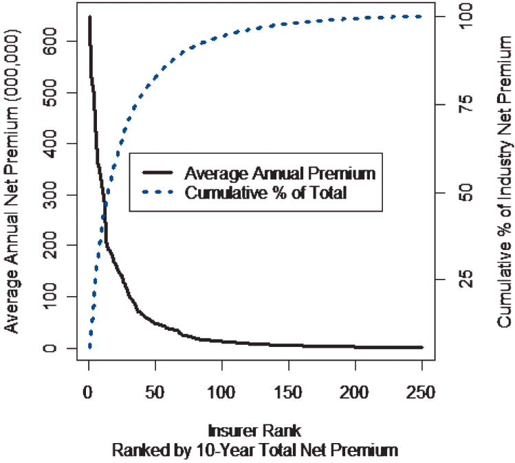
Let’s look at some graphic summaries of the data. Figure 1 shows the distribution of insurer sizes, ranked by 10-year total earned premium. It is worth noting that 16 of the insurers accounted for more than half of the total premium of the 250 insurers.

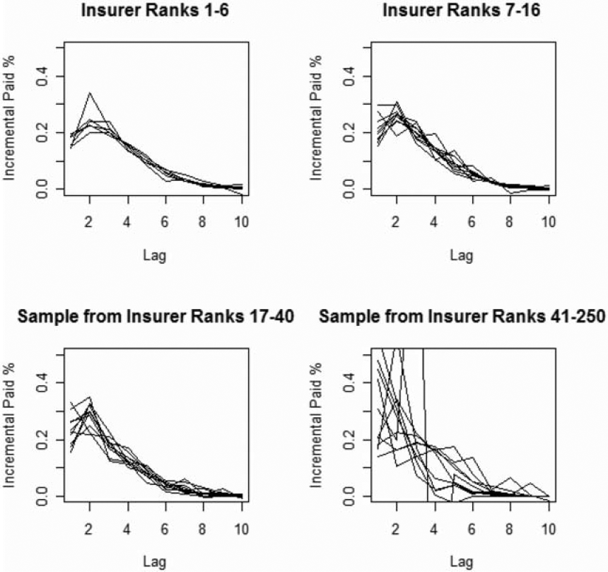
Figure 2 shows the variability of payment paths (i.e., proportion of total reported paid loss segregated by settlement lag) for the accident year 1986. This figure makes it clear that payment paths do vary by insurer. How much these differences can be attributed to systematic differences between insurers, versus how much can be attributed to random processes, is unclear at this point.

Figure 3 shows the aggregate payment patterns for four groups, each accounting for approximately one quarter of the total premium volume.

-
Insurers ranked 1–6, 7–16, 17–40, and 41–250 each accounted for about one quarter of the total premium.
-
Each plot represents approximately one quarter of the total premium volume.
-
The variability of the incremental paid loss factors increases as the size of the insurer decreases.
-
Segment 1—Insurers ranked 1–6, Segment 2—Insurers ranked 7–16, Segment 3—Insurers ranked 17–40, Segment 4—Insurers ranked 41–250.
-
There is no indication of any systematic differences in payout patterns by size of insurer.
3. A stochastic loss reserve model
The goal of this paper is to develop a loss reserving model that makes testable predictions, and to then actually perform the tests. Let’s start with a more detailed outline of how I intend to reach this goal.
-
The model for the expected payouts will be fairly conventional. It will be similar to the “Cape Cod” approach first published by Stanard (1985). This approach assumes a constant expected loss ratio across the 10-year span of the data.
-
Given the expected loss, the distribution of actual losses around the expected will be modeled by the collective risk model—a compound frequency and severity model. As mentioned above, this approach has precedents with Hayne (2003). This will conclude Section 3.
-
In Section 4, I will turn to estimating the parameters for the above models. The initial estimation method will be that of maximum likelihood.
-
I will then discuss testing the predictions of the model in Section 5. Initially, the tests will be on the same data that was used for fitting the models. (The tests on data in the 2001 Annual Statements will come later.) As mentioned above, the test will consist of calculating the percentiles of each of the observed loss payments and testing to see that those predictions are uniformly distributed.
As we proceed, I will focus on the 40 largest insurers. I do this because, in my judgment, the models are responding mainly to random losses for the smaller insurers. As we shall see, the results of the fitted models for the 40 largest insurers will form the basis for the Bayesian analysis that will be applied to each insurer, large and small. Implicit in this approach is the assumption that main systematic differences in the loss payment paths are somehow captured by the largest 40 insurers.
Let’s proceed.
Assume that the expected losses are given by the following model.
E[ Paid Loss AY,Lag]= Premium AY×ELR× Dev Lag
where
-
AY(1986 = 1,1987 = 2, . . .) is an index for accident year.
-
Lag = 1,2, . . . , 10 is the settlement lag reported after the beginning of the accident year.
-
Paid Loss is the incremental paid loss for the given accident year and settlement lag.
-
Premium is the earned premium for the accident year.
-
ELR is an unknown parameter that represents the expected loss ratio.
-
DevLag is an unknown parameter that depends on the settlement lag.
As with Stanard’s “Cape Cod” method, the ELR parameter will be estimated from the data.
The “Cape Cod” formula that I used to estimate the expected loss is by no means a necessary feature of this method. Other formulas, like the chain ladder model, can be used.
A common adjustment that one might make to Equation 1 is to multiply the ELR by a premium index to adjust for the “underwriting cycle.” I tried this, but it did not appreciably increase the accuracy of the predictions for this data and time period. Thus I chose to use the simpler model in this paper. But one should consider using a premium index in other circumstances.
Let XAY,Lag be a random variable for an insurer’s incremental paid loss in the specified accident year and settlement lag. Assume that XAY,Lag has a compound negative binomial (CNB) distribution, which I will now describe.
-
Let ZLag be a random variable representing the claim severity. Allow each claim severity distribution to differ by settlement lag.
-
Given E[Paid Loss]AY,Lag, define the expected claim count λAY,Lag by
λAY, Lag ≡E[ Paid loss AY, Lag ]/E[ZLag ]
This definition of the expected claim count may not correspond to the way an insurer actually counts claims. What is important is that it is consistent with the way the claim severity distribution is constructed. Our purpose is to describe the distribution of XAY,Lag.
-
Let NAY,Lag be a random variable representing the claim count. Assume that the distribution of NAY,Lag is given by the negative binomial distribution with mean λAY,Lag and variance λAY,Lag + c · λ2AY,Lag.
-
Then the random variable XAY,Lag is defined by XAY,Lag=ZLag,1+ZLag,2+⋯+ZLag,NAY,Lag
While the above defines how to express the random variable XAY,Lag in terms of other random variables NAY,Lag and ZLag, later on we will need to calculate the likelihood of observing xAY,Lag for various accident years and settlement lags. The details of how to do this are in the technical appendix. Here is a high-level overview of what will be done below.
- The distributions of ZLag were derived from data reported to ISO as part of its regular increased limits ratemaking activities. Like the substantial majority of insurers that report their data to ISO, the policy limit will be set to $1,000,000. The distributions varied by settlement lag with lags 5–10 having the highest severity. See Figure 4 below. For this application I discretized the distributions at intervals h, which depended on the size of the insurer. I chose h so the 214 (16,384) values spanned the probable range of losses for the insurer.

-
I selected the value of 0.01 for the negative binomial distribution parameter, c. The paper by Meyers Meyers (2006) analyzes Schedule P data for Commercial Auto and provides justification for this selection.
-
Using the Fast Fourier Transform (FFT), I then calculated the entire distribution of a discretized XAY,Lag, rounded to the nearest multiple of h. The use of Fourier Transforms for such calculations is not new. References for this in CAS literature include the papers by Heckman and Meyers (1983) and Wang (1998).
-
Whenever the probability density of a given observation xAY,Lag given E[Paid LossAY,Lag] was needed, I rounded the xAY,Lag to the nearest multiple of h and did the above calculation.
The resulting distribution function is denoted by:
CNB(xAY, Lag ∣E[ Paid loss AY, Lag ]).
This specifies the stochastic loss reserving model used in this paper. The parameters that depend on the particular insurer are the ELR and the 10 DevLag parameters. I will now turn to showing how to estimate these parameters, given the earned premiums and the Schedule P loss triangle.
Clark (2003) has taken a similar approach to loss reserve estimation. Indeed, I credit Clark for the inspiration that led to the approach taken in this section and the next. Clark used the Weibull and loglogistic parametric models where I used Equation 1 above. In place of the CNB distribution described above, Clark used what he calls the “overdispersed Poisson” (ODP) distribution.[1] He then estimated the parameters of his model by maximum likelihood. This is where I am going next.
4. Maximum likelihood estimation of model parameters
The data for a given insurer consists of earned premium by accident year, indexed by AY = 1, 2, . . . , 10, and a Schedule P loss triangle with losses {xAY,Lag} and Lag = 1, . . . ,(11 − AY). With this data, one can calculate the probability, conditional on the parameters ELR and DevAY,Lag, of obtaining the data by the following equation.
L({xAY, Lag })=∏10AY=1∏11−AYLag =1CNB(xAY, Lag ∣E[ Paid LossAY, Lag ])
Generally one calls L(·) the likelihood function of the data.
For this model, maximum likelihood estimation refers to finding the parameters ELR and DevLag that maximize Equation 4 (indirectly through Equation 1). There are a number of mathematical tools that one can use to do this maximization. The particular method I used is described in the Appendix.
After examining the empirical paths plotted in Figures 2 and 3, I decided to put the following constraints in the DevLag parameters.
-
Dev1 ≤ Dev2.
-
Devj ≥ Devj+1 for j = 2,3, . . . ,9.
-
Dev7/Dev8 = Dev8/Dev9 = Dev9/Dev10.
-
∑10i=1 Devi = 1.
The third set of constraints was included to add stability to the tail estimates. They also reduce the number of free parameters that need to be estimated from eleven to nine. The last constraint eliminated an overlap with the ELR parameter and maintained a conventional interpretation of that parameter.
Figure 5 plots the fitted payment paths for each of the 250 insurers. You might want to compare these payment paths with the empirical payment paths in Figure 2.
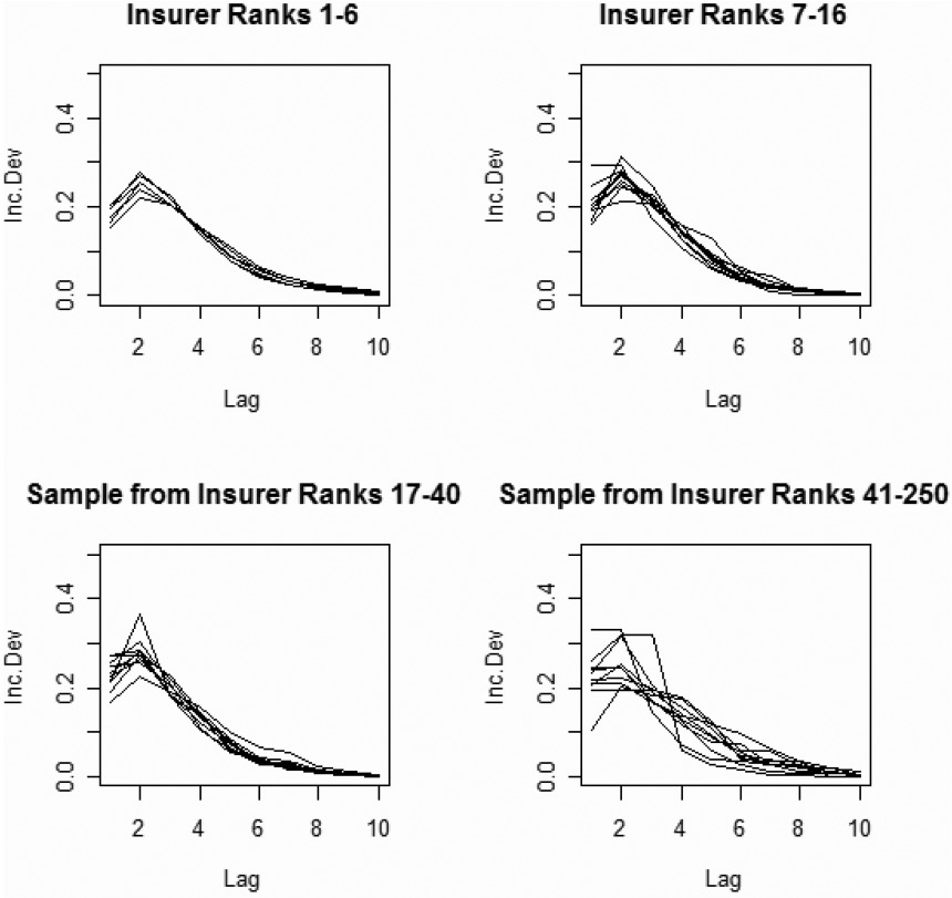
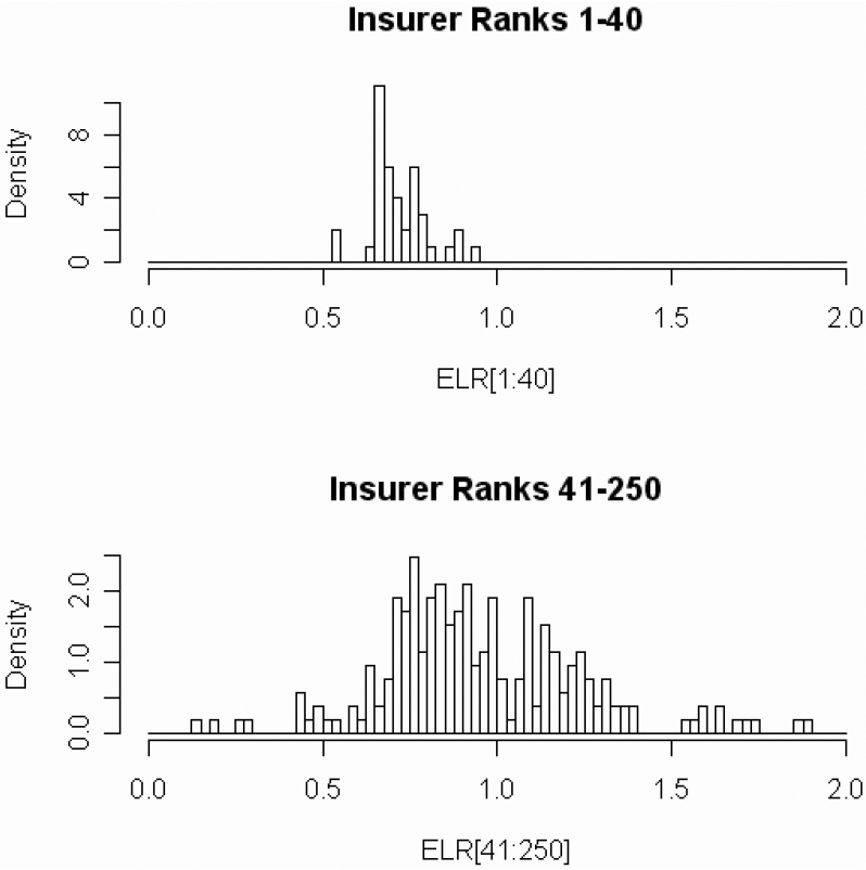
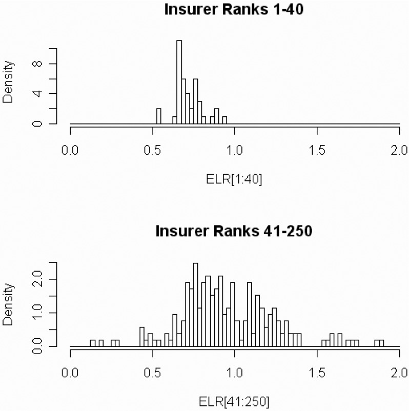
Figure 6 gives histograms of the 250 ELR estimates.
-
The samples are the same insurers as in Figure 2.
-
Note the wide variability of the fitted payment paths for the smallest insurers.
-
Note the high variability of the ELR estimates for the smallest insurers.
5. Testing the model
Given parameter estimates ELR and DevAY,Lag, one can use the model specified by Equations 1–3 above to calculate the percentile of any observation xAY,Lag by first calculating the expected loss, then the expected claim count, and finally the distribution of losses about the expected loss by the CNB distribution. Whatever the expected losses, accident year or settlement lag, the percentiles should be uniformly distributed. One can also include the calculated percentiles of several insurers to give a more conclusive test of the model.
The hypothesis that any given set of numbers has a uniform distribution can be tested by the Kolmogorov-Smirnov test. See, for example, Klugman, Panjer, and Willmot (KPW) (2004, 428) for a reference on this test. The test is applied in our case as follows. Suppose you have a sample of numbers, F1,F2, . . . ,Fn, between 0 and 1, sorted in increasing order. One then calculates the test statistic:
D=maxi|Fi−in+1|.
If D is greater than the critical value for a selected level α, we reject the hypothesis that the Fis are uniformly distributed. The critical values depend upon the sample size. Commonly used critical values are 1.22/ for α = 0.10,1.36/ for α = 0.05, and 1.63/ for α = 0.01.
Note that the Kolmogorov-Smirnov test should not be applied when testing the model with data that was used to fit the model.
A graphical way to test for uniformity is a p-p plot, which is sometimes called a probability plot. A good reference for this is KPW (2004, 424). The plot is created by arranging the observations F1,F2, . . . ,Fn in increasing order and plotting the points (i/(n + 1),Fi) on a graph. If the model is “plausible” for the data, the points will be near the 45° line running from (0,0) to (1,1). Let dα be a critical value for a Kolmogorov-Smirnov test. Then the p-p plot for a plausible model should lie within ±dα of the 45° line.
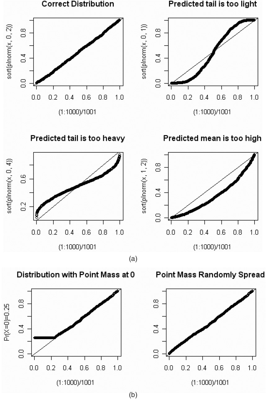
A nice feature of p-p plots is that they provide, to the trained eye, a diagnosis of problems that may arise from an ill-fitting model. Let’s look at some examples. Let x be a random sample of 1,000 numbers from a lognormal distribution with parameters μ = 0 and σ = 2. Let’s look at some p-p plots when we mistakenly choose a lognormal distribution with different μs and σs. On Figure 7(a), sort(plnorm(x,μ,σ)) on the vertical axis will denote the sorted Fis predicted by a lognormal distribution with parameters μ and σ.
-
On the first graph, μ and σ are the correct parameters, and the p-p plot lies on a 45° line as expected.
-
On the second graph, with σ = 1, the low predicted percentiles are lower than expected, while the high predicted percentiles are higher than expected. This indicates that the tails are too light.
-
On the third graph, with σ = 4, the low predicted percentiles are higher than expected, while the high predicted percentiles are lower than expected. This indicates that the tails are too heavy.
-
On the fourth graph, with μ = 1, almost all the predicted percentiles are lower than expected.
This indicates that the predicted mean is too high.
If a random variable X has a continuous cumulative distribution function F(x), the Fis associated with a sample {xi} will have a uniform distribution. There are times when we want to use a p-p plot with a random variable X, which we expect to have a positive probability at x = 0. The left side of Figure 7(b) shows a p-p plot for a distribution with Pr(X = 0) = 0.25. The Kolmogorov-Smirnov test is not applicable in this case. However, we can “transform” the Fis into a uniform distribution by multiplying Fi = F(xi) by a random number that is uniformly distributed whenever xi = 0. We can then use the Kolmogorov-Smirnov test of uniformity. The right side of Figure 7(b) illustrates the effect of such an adjustment. All of the p-p plots below will have this adjustment.
Now let’s try this for real.
Figure 8 gives a p-p plot for the percentiles predicted for the data that was used to fit each model for the top 40 insurers. Overall there were 2,200 (= 40 × 55) calculated percentiles. By examining Figure 8, we see that the fitted model has tails that are a bit too heavy.

Let me make a personal remark here. In my many years of fitting models to data, it is a rare occasion when a model passes such a test with data consisting of thousands of observations. I was delighted with the goodness of fit. Nevertheless, I investigated further to see what “went wrong.” Figure 9 shows p-p plots for the same data segregated by settlement lag. These plots appear to indicate that the main source of the problem is in the distributions predicted for the lower settlement lags.
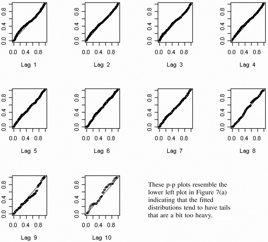
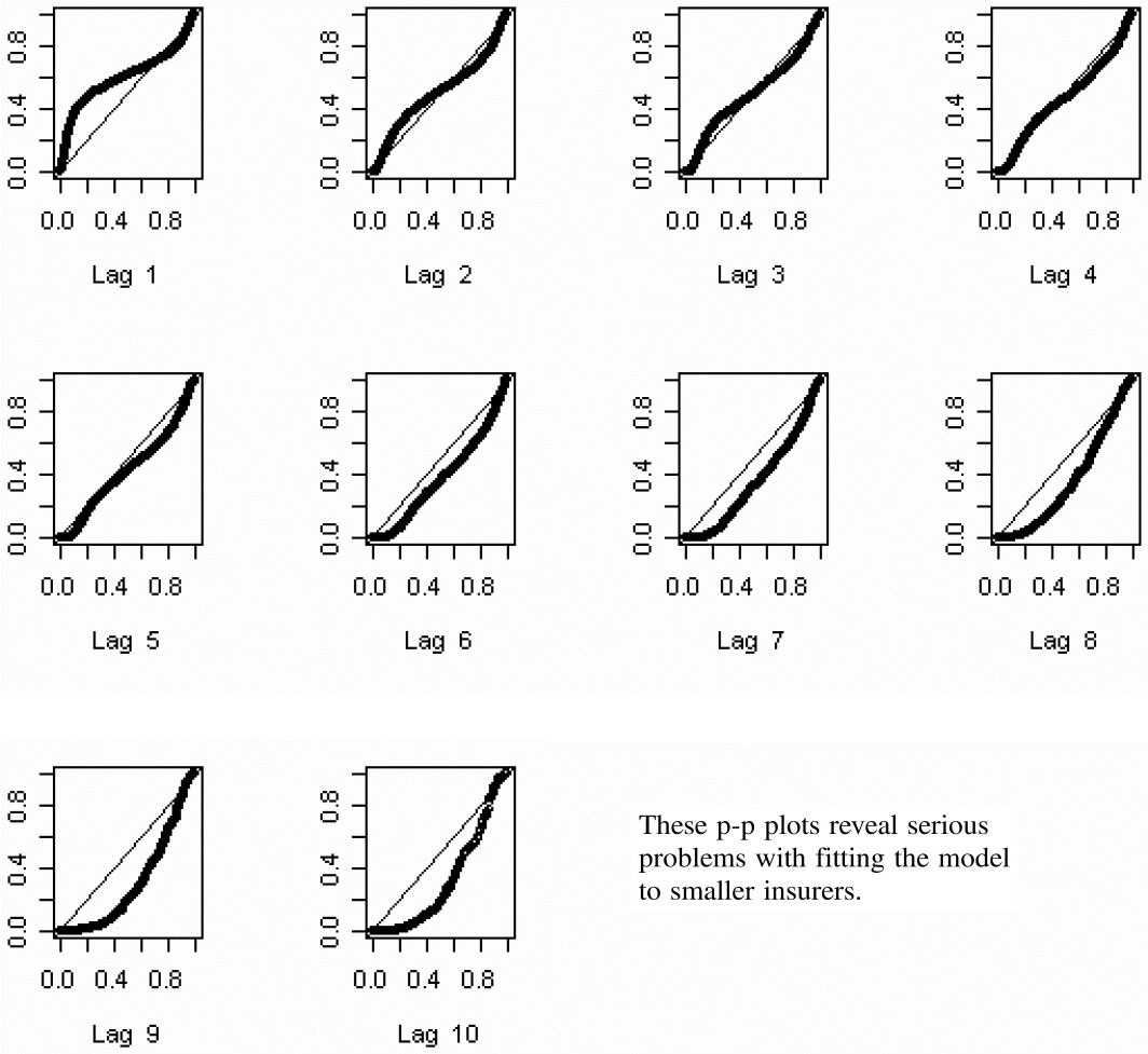
Figure 10 shows p-p plots for the percentiles predicted for the data used in fitting the smallest 210 insurers. Suffice it to say that these plots reveal serious problems with using this estimation procedure with the smaller insurers. I think the problem lies in fitting a model with nine parameters to noisy data consisting of 55 observations. On the other hand, the procedure appears to work fairly well for large insurers with relatively stable loss payment patterns. See Figures 2, 3, 5, and 6. I suspect the same problem with small insurers occurs with other many-parameter models, such as the chain ladder method.
6. Predicting future loss payments using Bayes’ Theorem
The failure of the model to predict the distribution of losses for the smaller insurers and the comparatively successful predictions of the model on larger insurers leads to the question: Is there any information that can be gained from the larger insurers that would be helpful in predicting the loss payments of the smaller insurers? That is the topic of this section.
Let ω = {ELR(ω),DevLag(ω),Lag = 1,2, . . . ,10} be a set of vectors that determine the expected losses in accordance with Equation 1. Let Ω be the set of all ωs. These models are distinguished only by the values of their parameters, and not by the assumptions or methods that were used to generate the parameters. Using Equation 4, one can combine each expected loss model with the parameters as assumptions underlying Equations 2 and 3 to calculate the likelihood of the given loss triangle {xAY,Lag}. Each likelihood can be interpreted as:
L=Probability{ data ∣ model }≡Pr{{xAY, Lag }∣ω}
Then using Bayes’ Theorem one can then calculate:
∝ Probability { data ∣ model }× Prior { model }.
Stated more mathematically:
Pr{ω∣{xAY, Lag }}∝Pr{{xAY, Lag }∣ω}×Pr{ω}.
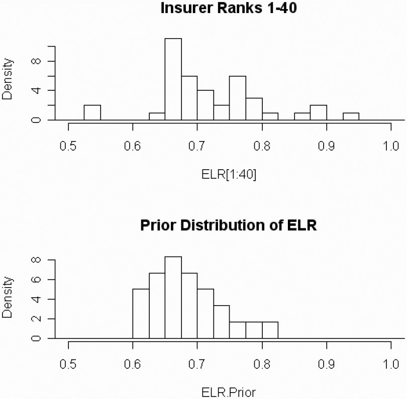
Each ω ∈ Ω will consist of forty {DevLag} combinations taken from maximum likelihood estimates of the top 40 insurers above. I judgmentally selected equal probabilities for each ω ∈ Ω. Each of the forty {DevLag} combinations will be independently crossed with nine potential ELRs starting with 0.600 and increasing by steps of 0.025 to a maximum of 0.800. Thus Ω has 360 parameter sets. I judgmentally selected the prior probability of the ELRs after an inspection of the distribution of maximum likelihood estimates. See Figure 11 and Table 1 below.
So we are given a loss triangle {xAY,Lag}, and we want to find a stochastic loss model for our data. Here are the steps we would take to do this.
-
Using Equation 4, calculate Pr{{xAY,Lag} | ω} for each ω ∈ Ω.
-
The posterior probability of each ω ∈ Ω is given by
Pr{ω∣{xAY, Lag }}=Pr{{xAY, Lag }∣ω}×Pr{ω}∑ω∈ΩPr{{xAY, Lag }∣ω}×Pr{ω}.
In words, the final stochastic model for a loss triangle is a mixture of all the models ω ∈ Ω, where the mixing weights are proportional to the posterior probabilities.
Here are some technical notes.
-
In doing these calculations for the 250 insurers, it happens that almost all the weight is concentrated on, at most, a few dozen models out of the original 360. So, instead of including all models in the original Ω, I sorted the models in decreasing order of posterior probability and dropped those after the cumulative posterior probability summed to 99.9%.
-
When calculating the final model for any of the top 40 insurers, I excluded that insurer’s parameters {DevLag} from Ω and added the parameters for the 41st largest insurer in its place. I did this to reduce the chance of overfitting.
The stochastic model of Equation 8 is not the end product. Quite often, insurers are interested in statistics such as the mean, variance, or a given percentile of the total reserve. I will now show how to use the stochastic model to calculate these “statistics of interest.”
At a high level, the steps for calculating the “statistics of interest” are as follows.
-
Calculate the statistic conditional on ω for each accident year and settlement lag of interest, i.e., the complement of the triangle AY = 2, . . . ,10, Dev = 12 − AY, . . . ,10.
-
Aggregate the statistic over the desired accident years and settlement lags for each ω.
-
Calculate the unconditional statistic by mixing (or weighting) the conditional statistics of Step 2, above, with the posterior probabilities of each model in Ω.
These steps should become clearer as we look at specific statistics. Let’s start with the expected value.
-
For each accident year and settlement lag, calculate the expected value for each ω using Equation 1. E[ Paid Loss AY,Lag∣ω]= Premium AY×ELR(ω)× Dev Lag (ω)
-
To get the total expected loss for each ω, sum the expected values over the desired accident years and settlement lags. E[ Paid loss ∣ω]=∑AY, Lag E[ Paid loss AY, Lag ∣ω].
-
The unconditional total expected loss is the posterior probability weighted average of the conditional total expected losses, with the posterior probabilities given by Equation 8. E[ Paid loss ]=∑ω∈ΩE[ Paid loss ∣ω]×Pr{ω∣{xAY, Lag }}.
Note that for each ω, the conditional expected loss will differ. Our next “statistic of interest” will be the standard deviation of these expected loss estimates. This should be of interest to those who want a “range of reasonable estimates.”
The first two steps are the same as those for finding the expected loss above. In the third step we calculate E[Paid Loss] as above but, in addition, we calculate the second moment:
-
SM[ˆE[ Paid loss ]]≡∑ω∈ΩE[ Paid loss ∣ω]2×Pr{ω∣{xAY, Lag }}
Then: Standard Deviation [ˆE[ Paid loss ]]=√SM[ˆE[ Paid loss ]]−E[ Paid loss ]2.
As the second example begins to illustrate, the three steps to calculating the “statistic of interest” can get complex.
Our third “statistic of interest” is the standard deviation of the actual loss. Before we begin, it will help to go over the formulas involved in finding the standard deviation of sums of losses.
First, recall from Equation 2 that our model imputes an expected claim count, λAY,Lag, by dividing the expected loss by the expected claim severity for the settlement lag.
Next recall the following bullet from the description of the CNB distribution above.
- Let NAY,Lag be a random variable representing the claim count. Assume that the distribution of NAY,Lag is given by the negative binomial distribution with mean λAY,Lag and variance λAY,Lag + c · λ2AY,Lag.
The negative binomial distribution can be thought of as the following process.
-
Select the random number χ from a gamma distribution with mean 1 and variance c.
-
Select NAY,Lag from a Poisson distribution with mean χ · λAY,Lag.
Consider two alternatives for applying this to the claim count for each settlement lag in a given accident year.
-
Select χ independently for each settlement lag.
-
Select a single χ and apply it to each settlement lag.
If one selects the second alternative, the multivariate distribution of {NAY,Lag} is called the negative multinomial distribution. This does not change the distribution of losses of an individual settlement lag. It does generate the correlation between the claim counts by settlement lag.
I will assume that the multivariate claim count for settlement lags within a given accident year has a negative multinomial distribution. The thinking behind this is that the χ is the result of an economic process that affects how many claims occur in a given year.
Clark (2006) provides an alternative method for dealing with correlation between settlement lags.
Let be the cumulative distribution for ZLag. Mildenhall (2006) shows that (stated in the notation of this paper) the distribution of has a CNB distribution with expected claim count and claim severity distribution
FZAY, Tot =10∑Lag =12−AYλAY, Lag ⋅FZLag /10∑Lag =12−AYλAY, Lag .
Now let’s describe the three steps to calculate the standard deviation of the actual loss.
-
For each accident year and settlement lag, calculate the expected claim count λAY,Lag(ω) using Equation 2.
-
The aggregation for each ω takes place in two steps.
a. Calculate the mean and variance of each accident year’s actual loss. E[ Paid LossAY∣ω]=λAY, Tot (ω)⋅E[ZAY, Tot ].Var[ Paid LossAY∣ω]=λAY, Tot (ω)⋅SM[ZAY, Tot ]+c⋅λAY, Tot (ω)2⋅E[ZAY, Tot ]2.
b. Sum the first and second moments over the accident years. E[ Paid Loss ∣ω]=∑AYE[ Paid LossAY∣ω].SM[ Paid Loss ∣ω]=∑⋯SM[ Paid LossAY∣ω].
-
E[PaidLoss]=∑ω∈ΩE[ Paid Loss ∣ω]×Pr{ω∣{xAY,Lag }}.SM[PaidLoss]=∑ω∈ΩSM[ Paid Loss ∣ω]×Pr{ω∣{xAY, Lag }}.StandardDeviation[PaidLoss]=√SM[ Paid Loss ]−E[ Paid Loss ]2.
The final “statistic of interest” is the distribution of actual losses. We are fortunate that the CNB distribution of each individual XAY,Lag is already defined in terms of its Fast Fourier Transform (FFT). To get the FFT of the sum of losses, we can simply multiply the FFTs of the summands. Other than that, the three steps are similar to those of calculating the standard deviation of the actual losses. To shorten the notation, let X denote Paid Loss.
-
For each accident year and settlement lag, calculate the expected claim count λAY,Lag(ω) using Equation 2.
-
The aggregation for each ω takes place in three steps.
a. Calculate the severity FFT Φ(→pAY, Tot ∣ω)=∑10Lag =12− AY λAY,Lag(ω)⋅Φ(→pLag ∣ω)/∑10Lag =12−AYλAY,Lag(ω) for each accident year, and then
b. calculate the accident year FFT Φ(→qAY, Tot ∣ω)=(1−c⋅(∑10Lag =12− AY λAY, Lag (ω))⋅(Φ(→pAY, Tot ∣ω)−1))−1/c for each accident year.
c. The FFT for the sum of all accident years is given by: Φ(→qω)=∏AYΦ(→qAY, Tot ∣ω)
-
The distribution of actual losses is obtained by inverting the FFT: Φ(→q)=∑ω∈ΩΦ(→qω)×Pr{ω∣{xAY, Lag }}.
See the Appendix for additional mathematical details of working with FFTs.
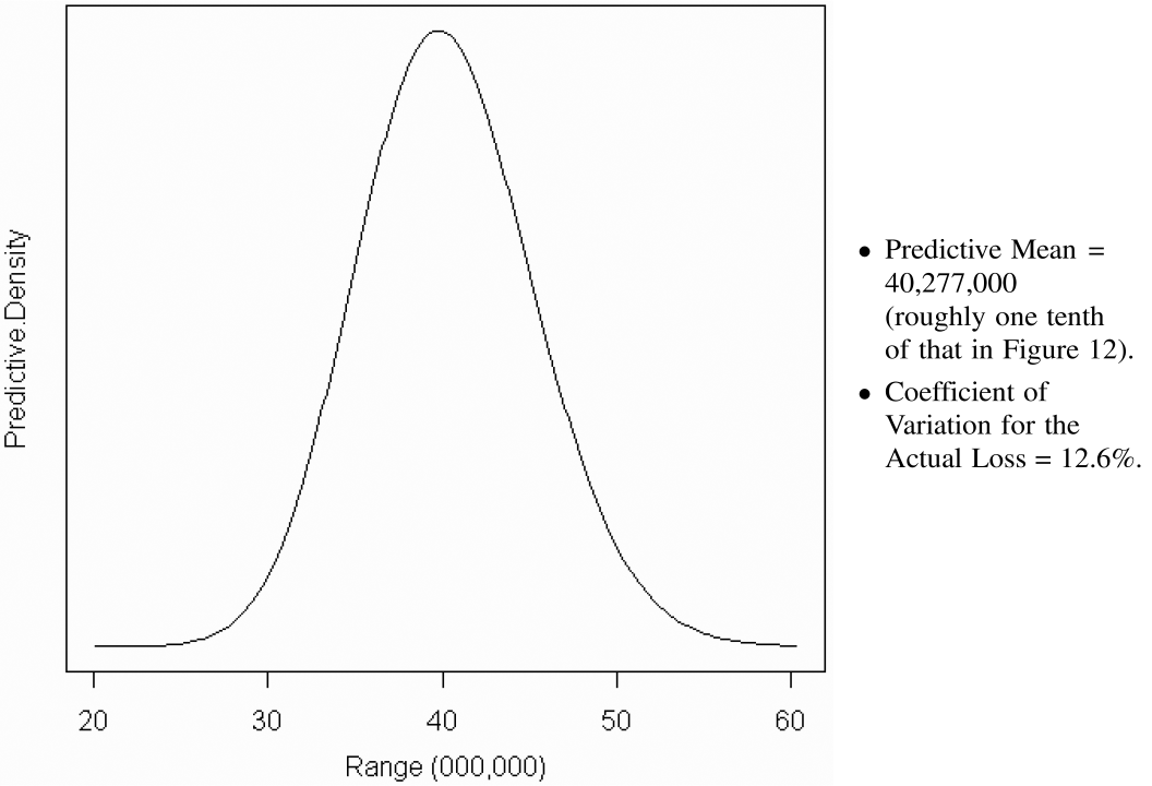
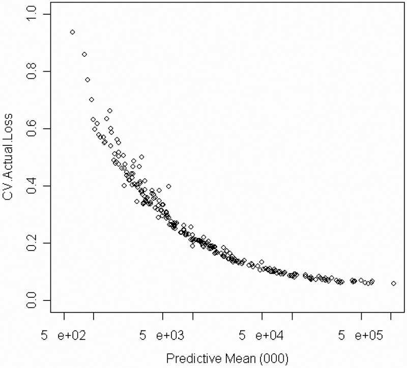
Figures 12 and 13 below show each of the three statistics for two insurers for the outstanding losses for accident years 2, . . . ,10 up to settlement lag 10. The insurer in Figure 12 has ten times the predictive mean reserve as the insurer in Figure 13. Figure 14 plots the predictive coefficient of variation against the predictive mean reserve. The decreased variability that comes with size should not come as a surprise. The absolute levels of variability will be interesting only if I can demonstrate that this methodology can predict the distribution of future results. That is where I am going next.
7. Testing the predictions
The ultimate test of a stochastic loss reserving model is its ability to correctly predict the distribution of future payments. While the distribution of future payments will differ by insurer, when one calculates the predicted percentile of the actual payment, the distribution of these predicted percentiles should be uniform.
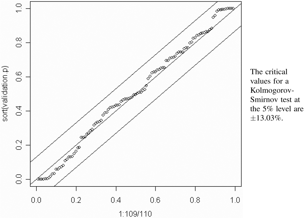
To test the model, we examined Schedule P from the 2001 NAIC Annual Statement. The losses reported in these statements contain six subsequent diagonals on the four overlapping years from 1992 through 1995. Earned premiums and losses in the overlapping diagonals for the 1995 and 2001 Annual Statements agreed in 109 of the 250 insurers, so I used these 109 insurers for the test.
Using the predictive distribution described in the last section, I calculated the predicted percentile of the total amount paid for the four accident years in the subsequent six settlement lags. These 109 percentiles should be uniformly distributed. Figure 15 shows the corresponding p-p plot and the confidence bands at the 5% level as determined by the Kolmogorov-Smirnov test. The plot lies well within that band. While we can never “prove” a model is correct with statistics, we gain confidence in a model as we fail to reject the model with such statistical tests. I believe this test shows that the Bayesian CNB model deserves serious consideration as a tool for setting loss reserves.

8. Comparing the predictive reserves with reported reserves
This section provides an illustration of the kind of analysis that can be done externally with the Bayesian methodology described in this paper. Readers should exercise caution in generalizing the conclusions of this section beyond this particular line of business in this particular time period.
This paper makes no attempt to pin down the methods used in setting the reported reserves. However, there are many actuaries that expect reported reserves to be more accurate than a formula derived purely from the paid data reported on Schedule P. As stated in the introduction to this paper, those who set those reserves have access to more information that is relevant to estimating future loss payments.
The comparisons below will be performed to two sets of insurers—the entire set of 250 insurers and the subset of 109 insurers for which the overlapping accident years 1992–1995 agree. Testing the latter will enable us to compare the predictions based on information available in 1995 with the incurred losses reported in 2001.
The first test looks at aggregates summed over all insurers in each set. Table 2 compares the predictions of this model with the actual reserves reported on the 1995 annual statement. The “actual reserve” is the difference between the total reported incurred loss, as of 1995 for the “initial” reserve, and 2001 for the “retrospective” reserve, minus the total reported paid loss, as of 1995.
For the 250 insurers, the reported initial reserve was 9.1% higher than the predictive mean. For the 109 insurers the corresponding percentage was 9.9%. The lowering of the percentage reserves from 1995 to 2001 to 2.4% suggests that for the industry, reserves were redundant for Commercial Auto in 1995.[2]
For the remainder of this section, let’s suppose that the expected value of the Bayesian CNB model described above is the “best estimate” of future loss payments. From the above, there are two arguments supporting that proposition.
-
Figure 15 in Section 7 above shows that the Bayesian CNB model successfully predicted the distribution of payments for the six years after 1995 well within the usually accepted statistical bounds of error.
-
The final row of Table 2 shows that the expected value predicted by the Bayesian CNB model, in aggregate, comes closer to the 2001 reserve than did the reported reserves for 1995.
Now let’s examine some of the implications of this proposition for reported reserves.
There are many actuaries who argue that reported reserves should be somewhat higher than the mean. See, for example, Paragraph 2.17 on page 5 of Report of the Insurer Solvency Working Party of the International Actuarial Association (2004). Related to this, I recently saw a working paper by Grace and Leverty (n.d.) that tests various hypotheses on insurer incentives.
If insurers were deliberately setting their reserves at some conservative level, we would expect to see that the reported reserves are at some moderately high percentile of the predictive distribution. Figure 16 shows that some insurers appear to be reserving conservatively. But there are also many insurers for which the predictive percentile of the reported reserve is below 50%. But by 2001, the percentiles of the retrospective reserve for 1995 were close to being uniformly distributed.

-
The greater number of insurers reserved above the 50th percentile indicates that some insurers have conservative estimates of their loss reserves posted in 1995.
-
The right side of this figure shows that the spread of the reserve percentiles spans all insurer sizes.
If there is a bias in the posted reserves, we would see corrections in subsequent years. The 109 insurers for which we have subsequent development provide data to test potential bias. To perform such a test, I divided the 109 insurers into two groups. The first group consisted of all insurers that posted reserves in 1995 that were lower than their predictive mean. The second group consisted of all insurers that posted reserves higher than their predictive mean.
As Figure 17 and Table 3 show, the first group shows an upward adjustment and the second group shows a more pronounced downward adjustment. The plots show that we cannot attribute these adjustments to only a few insurers. However, there are some insurers in the first group that show a downward adjustment, and other insurers in the second group that show an upward adjustment.

The fact that the total adjustments only go part way to the predictive mean suggests that some insurers may be able to make more accurate estimates with access to information that is not provided on Schedule P.
9. Summary and conclusions
This paper demonstrates a method, which I call the Bayesian CNB model, for estimating the distribution of future loss payments of individual insurers. The main features of this method are as follows.
-
The stochastic loss reserving model is based on the collective risk model. While other stochastic loss reserving approaches make use of the collective risk model, this approach uses it as an integral part of estimating the parameters of the model.
-
Predicted loss payments are derived from a Bayesian methodology that uses the results of large, and presumably stable, insurers as its “prior information.” While insurers do indeed differ in their claim payment practices, the underlying assumption of this methodology is that these differences are reflected in this collection of large insurers. This paper demonstrates that using prior information derived from large insurers, together with the CNB model for the stochastic losses, makes this method applicable to all insurers, both large and small.
-
Loss reserving models should be subject to testing their predictions on future payments. Tests on a single insurer are often inconclusive because of the volatile nature of the loss reserving process. But it is possible to test a stochastic loss reserving method on several insurers simultaneously by comparing its predicted percentiles of subsequent losses to a uniform distribution. This paper tests its model on 109 insurers and finds that its predictions are well within the statistical bounds expected for a sample of this size.
-
By making the assumption that the Bayesian CNB model provides the “best estimate” of future loss payments, the analysis in this paper suggested that there are some insurers that post reserves conservatively, while others post reserves with a downward bias. Readers should exercise caution in generalizing these conclusions beyond this particular line of business in this time period.
While this paper did not address the tail when a significant amount of losses are to be paid after 10 years, I do have some suggestions on how to use this approach when the tail extends beyond 10 years. First, the DevLag parameters in each ω could be extended further based on either analysis or the judgment of the insurer. The parameters for the later lags may differ even if the parameters for the earlier lags are identical. The data in Schedule P contains the sum of losses paid for all prior years. If the insurer has premium information from the prior years, the methods described in this paper could be used to calculate the distribution of that sum conditional on each model ω, and hence contribute to the estimation of the posterior probability of each model ω.
I view this paper as an initial attempt at a new method for stochastic loss reserving. To gain general acceptance, this approach should be tested on other lines of insurance and by other researchers. The data required to do such studies consist of Schedule Ps that American insurers are required to report to regulators, and claim severity distributions. This information can be obtained from vendors. AM Best compiles the Schedule P information. ISO fits claim severity distributions for many lines of insurance.
This method requires considerable statistical and actuarial expertise to implement. It also takes a lot of work. In this paper, I have tried to make the case that we should expect that such efforts could yield fruitful results.