Estimation and Robustness of Linear Mixed Models in Credibility Context

1. Introduction

Credibility theory is a method to predict the future exposures of a risk entity based on past information. In statistics, the credibility data can be treated as longitudinal data, and the development of credibility theory has been closely linked to the longitudinal data model. Frees, Young, and Lou (1999) has demonstrated the implementation of the linear mixed model under the classical credibility framework. The implementation of the generalized linear mixed model, which is an extension of the linear mixed model, has been proposed by Antonio and Beirlant (2006). Although only independent error structure has been considered in both literatures, the longitudinal data interpretation suggests additional techniques that actuaries can use in credibility rate making.

Later developments of credibility theory have considered the correlation between error terms. For instance, Cossette and Luong (2003) employed the regression credibility model, which can be regarded as a special form of the linear mixed model, to catch the random effects and within-panel correlation structure, and used weighted least squares method to estimate the variance covariance parameters. Lo, Fung, and Zhu (2006) and Lo, Fung, and Zhu (2007) proposed the generalized estimating equations (GEE) to handle the correlated error structure and estimate the variance of the random components under the regression credibility model. The methods in those papers have been justified by empirical studies.

In this paper, our attention is given to the linear mixed modeling in credibility context under Hachemeister’s model and Dannenburg’s model while taking into account both independent and correlated error structures. Maximum likelihood (ML) and restricted maximum likelihood (REML) methods are used to estimate the variance covariance parameters, where the random components are regarded as normally distributed. The performance of the ML and REML estimators are compared with the classical Hachemeister’s and Dannenburg’s estimators in simulation studies, when the error terms are normally distributed and non-normally distributed. In both situations, it can be shown that the ML that an REML approaches has clear advantages over its alternatives.

The structure of this paper is as follows. In Section 2, the regression credibility model is specified. Several commonly used error structures for modeling the observations of a risk entity are introduced. Section 3 gives a brief introduction on ML and REML methods and their applications to the linear mixed model. The estimation of the structural parameters in Hachemeister’s and Dannenburg’s two-way crossed classification models are studied in Sections 4 and 5. In both sections, a brief introduction of the credibility model and classical estimation method is given, then two simulation studies are presented to examine the performance of the proposed ML and REML approaches. The first study tests the performance of ML and REML approaches when the observations are normally distributed. The second study tests the performance of ML and REML approaches when the observations are lognormally distributed, i.e., the normality assumption is violated. A few concluding remarks are given in the last section. It can be shown that enormous discrepancies of the performance of the credibility estimator for the credibility factors and future exposure between the classical estimation approach and the ML, REML approaches occur in both Dannenburg’s model and Hachemeister’s model. For instance, when the error terms follow multivariate normal distribution, the mean squared errors of the classical estimators for future exposure are a few hundred times higher than the counterpart in the proposed ML approach.

2. Model specification

2.1. Regression credibility model

In this paper, we employ the regression credibility model which is proposed by Hachemeister (1975). It is a specific form of a linear mixed model that can help us capture within-panel correlation. The regression model has the following form:

\[ \mathbf{y}_{i}=\mathbf{X}_{i} \boldsymbol{\beta}_{i}+\varepsilon_{i}, \quad i=1,2, \ldots, n . \tag{1} \]

Each element \(y_{i j}\) in the \(r_i \times 1\) vector \(\mathbf{y}_i\) corresponds to the observed value with regard to risk entity \(i\) in the \(j\) th observation period. The design matrix \(\mathbf{X}_i\), of dimension \(r_i \times m\), enters the model as a known constant matrix. The dimension of the vector of regression coefficients \(\boldsymbol{\beta}_i\) is \(m . \boldsymbol{\beta}_i \mathrm{~s}\) are assumed to be independent and normally distributed, with common mean \(\boldsymbol{\beta}\) and variance covariance matrix \(\mathbf{F}\) for all \(i\). The error vectors \(\varepsilon_i \mathrm{~s}\) are taken to be independently distributed from a normal distribution with mean \(\mathbf{0}\) and variance covariance matrix \(\sigma^2 \mathbf{V}_i=\sigma^2 \mathbf{W}_i^{-1 / 2} \boldsymbol{\Gamma}_i \mathbf{W}_i^{-1 / 2}\), where \(\mathbf{W}_i^{-1 / 2}\) is a diagonal weight matrix of known constants and \(\boldsymbol{\Gamma}_i\) is a correlation matrix. Here we assume \(\Gamma_i\), which describes the correlation between the error terms \(\varepsilon_{i j}\) s for entity \(i\), to be positive definite and depends on some fixed unknown parameters which are to be estimated. Aided by the specifications stated above, readers may easily derive the following about \(\mathbf{y}_i\):

(a) \(\mathbf{y}_i\) and \(\mathbf{y}_j\) are statistically independent for \(i \neq j\);
(b) \(\mu_i=E\left(\mathbf{y}_i\right)=\mathbf{X}_i \boldsymbol{\beta}\);
(c) \(\mathbf{V}\left(\mathbf{y}_i\right)=\mathbf{X}_i \mathbf{F} \mathbf{X}_i^{\prime}+\sigma^2 \mathbf{W}_i^{-1 / 2} \boldsymbol{\Gamma}_i \mathbf{W}_i^{-1 / 2}\).

Hachemeister (1975) and Rao (1975) give the linear Bayes estimator for β_i, which minimizes the mean-squared error losses. This estimator takes the following form:

\[ \hat{\boldsymbol{\beta}}_{i}^{(\mathrm{B})}=\mathbf{Z}_{i} \hat{\boldsymbol{\beta}}_{i}^{(\mathrm{GLS})}+\left(\mathbf{I}-\mathbf{Z}_{i}\right) \boldsymbol{\beta}, \tag{2} \]

where \(\mathbf{Z}_i\) is the credibility matrix, \(\hat{\boldsymbol{\beta}}_i^{(\mathrm{GLS})}\) is the generalized least squares estimator for \(\boldsymbol{\beta}_i\), and we have

\[ \mathbf{Z}_{i}=\mathbf{F}\left[\mathbf{F}+\sigma^{2}\left(\mathbf{X}_{i}^{\prime} \mathbf{V}_{i}^{-1} \mathbf{X}_{i}\right)^{-1}\right]^{-1} ,\tag{3} \]

\[ \hat{\boldsymbol{\beta}}_{i}^{(\mathrm{GLS})}=\left(\mathbf{X}_{i}^{\prime} \mathbf{V}_{i}^{-1} \mathbf{X}_{i}\right)^{-1} \mathbf{X}_{i}^{\prime} \mathbf{V}_{i}^{-1} \mathbf{y}_{i} . \tag{4} \]

As we can see from the above, in order to get the estimation of \(\boldsymbol{\beta}_i\), we have to estimate the parameters \(\sigma^2, \rho, \boldsymbol{\beta}\), and \(\mathbf{V}_i\). The accuracy of the estimation of these parameters can largely affect the estimation efficiency for \(\boldsymbol{\beta}_i\).

2.2. Several commonly used error structures

The moving average (MA), autoregressive (AR), and exchangeable types of error are commonly used to model the correlation structure of observations within a risk entity. Those structures have certain simplicity, and by using relatively few unknown parameters they can capture the correlation structure well. Therefore, under credibility frameworks, we could use all these correlation structures to model the correlation between error terms. However, in our empirical studies we would like to only incorporate the MA(1) and the exchangeable error correlation structures under each credibility framework for brevity.

2.2.1. Moving average correlation structure

For an MA( \(q\) ) process, the correlation between the errors \(\varepsilon_j\) and \(\varepsilon_k\) can be written as

\[ \Gamma_{j k}=\left\{\begin{array}{ll} 1, & \text { for } \quad j=k \\ \rho_{|j-k|}, & \text { for } \quad 0<|j-k| \leq q, \\ 0, & \text { otherwise.} \end{array}\right. \]

For instance, the correlation matrix \(\left(\Gamma_{j k}\right)_{n \times n}\) of the MA(1) takes the explicit form of

\[ \Gamma=\left[\begin{array}{lllll} 1 & \rho & 0 & \cdots & 0 \\ \rho & 1 & \rho & \ddots & \\ 0 & \rho & 1 & \ddots & \\ & \ddots & \ddots & \ddots & \\ 0 & \cdots & 0 & \rho & 1 \end{array}\right] . \]

2.2.2. Autoregressive correlation structure

AR(q) is given by the equation

\[ \varepsilon_{t}=\sum_{i=1}^{q} \varphi_{i} \varepsilon_{t-i}+e_{t} . \]

As we can see there is no simple form for the correlation matrix when \(q\) gets large. Therefore AR(1) is the most commonly used model. For the AR(1) model, the correlation matrix \(\left(\Gamma_{j k}\right)_{n \times n}\) for the random errors \(\varepsilon_t \mathrm{~s}\) can be written in the following form:

\[ \Gamma=\left[\begin{array}{ccccc} 1 & \rho & \rho^{2} & \cdots & \rho^{n-1} \\ \rho & 1 & \rho & \ddots & \\ \rho^{2} & \rho & 1 & \ddots & \\ & \ddots & \ddots & \ddots & \\ \rho^{n-1} & \cdots & \rho^{2} & \rho & 1 \end{array}\right] . \]

2.2.3. Exchangeable correlation structure

The exchangeable type of correlation is also known as the uniform correlation. The correlation matrix \(\left(\Gamma_{j k}\right)_{n \times n}\) of the exchangeable type of error can be written as:

\[ \Gamma_{j k}=\left\{\begin{array}{ll} 1, & \text { for } \quad j=k,\\ \rho, & \text { otherwise.} \end{array}\right. \]

Therefore the exchangeable correlation matrix takes the explicit form of

\[ \Gamma=\left[\begin{array}{lllll} 1 & \rho & \rho & \cdots & \rho \\ \rho & 1 & \rho & \ddots & \\ \rho & \rho & 1 & \ddots & \\ & \ddots & \ddots & \ddots & \\ \rho & \cdots & \rho & \rho & 1 \end{array}\right] . \]

3. The ML and REML methods

In the regression credibility model, the variance and covariance parameters can be estimated using the well-known maximum likelihood (ML) and the restricted maximum likelihood (REML) estimation methods. As we all know that maximum likelihood estimators are obtained by maximizing the likelihood function, the restricted maximum likelihood has been proposed by modifying the maximum likelihood by partitioning the likelihood under normality into two parts, one of which is free of fixed effects. The restricted maximum likelihood estimators can be obtained by maximizing that part. While preserving the good properties of the ML estimators, the REML estimators have an additional property, which is to reduce the analysis variance for many, if not all, balanced data. Because both ML and REML methods are common statistical methods, detailed introduction is omitted in this paper.

From our assumption, the error vectors, \(\varepsilon_i\), and regression coefficient vectors, \(\boldsymbol{\beta}_i\), are normally distributed. This implies \(\mathbf{y}_i\) follows a multivariate normal distribution with derivable mean and variance covariance matrix

\[ \mathbf{y}_{i} \sim N\left(\mathbf{X}_{i} \boldsymbol{\beta}, \mathbf{X}_{i} \mathbf{F} \mathbf{X}_{i}^{\prime}+\sigma^{2} \mathbf{W}_{i}^{-1 / 2} \boldsymbol{\Gamma}_{i} \mathbf{W}_{i}^{-1 / 2}\right), \]

where \(\mathbf{X}_i \boldsymbol{\beta}\) is the fixed effect component of the linear mixed model. Hence we can derive the log likelihood and the restricted log likelihood function of \(\mathbf{y}_i\). They have been shown as

\[ L_{\mathrm{ML}}=c_{1}-\frac{1}{2} \sum_{i=1}^{n} \log \left|\mathbf{V}\left(\mathbf{y}_{i}\right)\right|-\frac{1}{2} \sum_{i=1}^{n} \mathbf{r}_{i}^{\prime} \mathbf{V}\left(\mathbf{y}_{i}\right) \mathbf{r}_{i}, \tag{5} \]

\[ \begin{aligned} L_{\mathrm{REML}}= & c_{2}-\frac{1}{2} \sum_{i=1}^{n} \log \left|\mathbf{V}\left(\mathbf{y}_{i}\right)\right| \\ & -\frac{1}{2} \log \left(\sum_{i=1}^{n}\left|\mathbf{X}_{i}^{\prime} \mathbf{V}_{i}^{-1} \mathbf{X}_{i}\right|\right)-\frac{1}{2} \sum_{i=1}^{n} \mathbf{r}_{i}^{\prime} \mathbf{V}\left(\mathbf{y}_{i}\right) \mathbf{r}_{i}, \end{aligned} \tag{6} \]

where

\[ \begin{aligned} \mathbf{r}_{i}= & \mathbf{y}_{i}-\mathbf{X}_{i}\left(\sum_{i=1}^{n} \mathbf{X}_{i}^{\prime} \cdot \mathbf{V}^{-1}\left(\mathbf{y}_{i}\right) \cdot \mathbf{X}_{i}\right)^{-1} \\ & \times\left(\sum_{i=1}^{n} \mathbf{X}_{i}^{\prime} \cdot \mathbf{V}^{-1}\left(\mathbf{y}_{i}\right) \cdot \mathbf{y}_{i}\right), \end{aligned} \]

and c₁, c₂ are appropriate constants.

We define the vector \(\boldsymbol{\alpha}\) which contains all of the parameters of interest. For example \(\boldsymbol{\alpha}= \left(\theta_{11}, \theta_{12}, \ldots, \theta_{m m}, \sigma^2, \rho\right)^{\prime}\), where \(\theta_{11}, \theta_{12}, \ldots, \theta_{m m}\) indicate the entries that specify the covariance matrix \(\mathbf{F}\). We could solve \(\boldsymbol{\alpha}\) by maximizing the log likelihood function with regard to \(\boldsymbol{\alpha}\) or by solving the score function

\[ \frac{\partial L_{\mathrm{ML}}}{\partial \boldsymbol{\alpha}}=0 \]

for the ML approach, and

\[ \frac{\partial L_{\mathrm{REML}}}{\partial \boldsymbol{\alpha}}=0 \]

for the REML approach. More details about the derivation of the likelihood and restricted likelihood functions, fixed and random effects, estimates of the variance and covariance components can be found in Laird and Ware (1982), McCulloch (1997), and Verbeke and Molenberghs (2000).

Computationally there are various ways to obtain the ML and the REML estimators, such as the Newton-Raphson method and the simplex algorithm. Details of those methods can be found in Lindstrom and Bates (1988) and Nelder and Mead (1965). There are also many statistical packages available that can be used to perform such estimation, such as Matlab, R, S+ and SAS.

4. Parameter estimation in Hachemeister’s model

4.1. Hachemeister’s model and method

Hachemeister’s model also known as the regression credibility model was proposed by Hachemeister (1975). It has the form

\[ E\left[\mathbf{y}_{i}(\Theta)\right]=\mathbf{X}_{i}^{\prime} \boldsymbol{\beta}_{i}, \quad i=1,2, \ldots, n, \tag{7} \]

where \(\Theta\) denotes the unobservable risk characteristic associated with each risk entity, and the dimension of \(\boldsymbol{\beta}_i\) is \(m\). We have

\[ \operatorname{Var}\left(\mathbf{y}_{i} \mid \Theta\right)=s^{2}(\Theta) \mathbf{W}_{i}^{-1}. \]

The credibility factor matrix stated in Hachemeister (1975) is

\[ \mathbf{Z}_{i}=\left(\mathbf{F X}_{i}^{\prime} \mathbf{W}_{i} \mathbf{X}_{i}+\sigma^{2} \mathbf{I}\right)^{-1} \mathbf{F} \mathbf{X}_{i}^{\prime} \mathbf{W}_{i} \mathbf{X}_{i} . \tag{8} \]

A weighted least squares estimate of β can be obtained by:

\[ \hat{\boldsymbol{\beta}}=\left(\mathbf{X}^{\prime} \mathbf{W X}\right)^{-1} \mathbf{X}^{\prime} \mathbf{W y} . \tag{9} \]

where

\[ \mathbf{X}=\left[\begin{array}{c} \mathbf{X}_{1} \\ \mathbf{X}_{2} \\ \vdots \\ \mathbf{X}_{n} \end{array}\right] \quad \text { and } \quad \mathbf{y}=\left[\begin{array}{c} \mathbf{y}_{1} \\ \mathbf{y}_{2} \\ \vdots \\ \mathbf{y}_{n} \end{array}\right] \tag{10} \]

are two large single unites, formed by the design matrices and the vectors of observations respectively, and

\[ \mathbf{W}=\left[\begin{array}{cccc} \mathbf{W}_{1} & & & \mathbf{0} \\ & \mathbf{W}_{2} & & \\ & & \ddots & \\ \mathbf{0} & & & \mathbf{W}_{n} \end{array}\right] \text {, } \tag{11} \]

is constructed with individual exposure matrices as building blocks along the principal diagonal.

An unbiased estimator of σ² takes the form

\[ \begin{aligned} \hat{\sigma}^{2} & =n^{-1} \sum_{i=1}^{n} \hat{\sigma}_{i}^{2} \\ & =n^{-1}(n-m)^{-1} \sum_{i=1}^{n}\left(\mathbf{y}_{i}-\mathbf{X}_{i}^{\prime} \hat{\boldsymbol{\beta}}_{i}\right)^{\prime} \mathbf{W}_{i}\left(\mathbf{y}_{i}-\mathbf{X}_{i}^{\prime} \hat{\boldsymbol{\beta}}_{i}\right), \end{aligned} \tag{12} \]

where \(\hat{\boldsymbol{\beta}}_i\) is the weighted least square estimator for \(\mathbf{b}\left(\theta_i\right)\). The estimator for the covariance matrix \(\mathbf{F}\) is somewhat more complex. Define

\[ \mathbf{G}=\left(\mathbf{X}^{\prime} \mathbf{W} \mathbf{X}\right)^{-1} \sum_{i=1}^{n}\left(\mathbf{X}_{i}^{\prime} \mathbf{W}_{i} \mathbf{X}_{i}\right)\left(\hat{\boldsymbol{\beta}}_{i}-\hat{\boldsymbol{\beta}}\right)\left(\hat{\boldsymbol{\beta}}_{i}-\hat{\boldsymbol{\beta}}\right)^{\prime}, \tag{13} \]

\[ \begin{aligned} \mathbf{\Pi}= & \mathbf{I}-\sum_{i=1}^{n}\left(\mathbf{X}^{\prime} \mathbf{W} \mathbf{X}\right)^{-1}\left(\mathbf{X}_{i}^{\prime} \mathbf{W}_{i} \mathbf{X}_{i}\right)\left(\mathbf{X}^{\prime} \mathbf{W} \mathbf{X}\right)^{-1} \\ & \times\left(\mathbf{X}_{i}^{\prime} \mathbf{W}_{i} \mathbf{X}_{i}\right). \end{aligned} \tag{14} \]

The unbiased estimator for F is

\[ \mathbf{C}=\Pi^{-1}\left[\mathbf{G}-(n-1)\left(\mathbf{X}^{\prime} \mathbf{W} \mathbf{X}\right)^{-1} \hat{\sigma}^{2}\right] . \tag{15} \]

Since F is symmetric, we can take our estimator as

\[ \hat{\mathbf{F}}=\left(\mathbf{C}+\mathbf{C}^{\prime}\right) / 2 . \tag{16} \]

4.2. Empirical studies

To estimate the structural parameters in Hachemeister’s model, we can use R, which is handy, user-friendly, and freely available from the internet. The simulation results we show in this section are obtained by using the subroutine lme in R.

In this section, we use two approaches to estimate the structural parameters.

1. Hachemeister: The classical Hachemeister estimators are computed.

2. ML: The maximum likelihood estimation is used to compute the structural parameters. Two ML estimators are used in this paper. They are linked with the independent and exchangeable error structures and are denoted by ML-I and ML-EX respectively.

From the simulation results, the performance of the ML approach and the REML approach is quite close. None of them performs universally better than the other. Therefore, for the sake of brevity, we only show the results of the ML approach.

In this part, two studies have been considered. Study 1 allows us to compare the performances of the ML estimator and Hachemeister’s estimator when the joint distribution of the observations in each contract is multivariate normal. The ML estimators are associated with different error structures, namely, independent and exchangeable error structure. Study 2 assesses the estimation efficiency of the ML estimator and Hachemeister’s estimator when the joint distribution of the observations in each contract is not multivariate normal, but multivariate log-normal. The number of replicates in each study is 500.

4.2.1. Study 1

In the simulation studies under Hachemeister’s framework, the number of entities n is set to be 25, and the number of observations in contract i is set to be 5 for each entity. The parameter values are taken as follows:

\[ \begin{aligned} \boldsymbol{\beta} & =(20,10)^{\prime}, \quad \sigma^{2}=4^{2}, \quad \theta_{11}=3^{2}, \\ \theta_{12} & =4, \quad \theta_{22}=3^{2} . \end{aligned} \]

Here \(\theta_{11}, \theta_{22}\) are the diagonal elements of \(\mathbf{F}\), while \(\theta_{12}\) is the off-diagonal element of \(\mathbf{F}\). Each weighting element \(w_{i j}\) is generated from a Poisson distribution with its mean \(\lambda_i\) following a uniform distribution defined in the interval \((5,100)\). The explanatory variable \(x_{i j 1}\) is set to be 1 , while \(x_{i j 2}\) is simulated from the normal distribution with variance 5 and around the mean level which is uniformly selected from the interval \((-5,5)\).

As for the simulation results, we show the bias and mean square error (MSE) of Hachemeister’s and ML for \(\beta_{i 1}, \beta_{i 2}, Z_{i 11}, Z_{i 12}, Z_{i 21}, Z_{i 22}, \theta_{11}, \theta_{12}\), \(\theta_{22}\) and \(\sigma^2\).

Table 1 is associated with an independent error structure, while Table 2 is associated with an MA(1) error structure. As we can see, while the unbiased property of Hachemeister’s estimator for the variance and covariance parameters is reasonably well exhibited, the huge discrepancies of the performance of the credibility estimators for \(\boldsymbol{\beta}_i\) and \(\mathbf{Z}_i\) between the ML method and Hachemeister’s method occur.

Notice that the mean squared error in estimating \(\boldsymbol{\beta}_i\) is impressively low for the ML method under both the independent and the MA(1) error structures. Judging from the credibility formula for computing \(\boldsymbol{\beta}_i\), the accuracy of the estimation for \(\boldsymbol{\beta}_i\) largely depends on the accuracy in estimating the credibility factor \(\mathbf{Z}_i\). The estimation of \(\mathbf{Z}_i\) relies on the estimation of the variance and covariance parameters. Thus, the mean squared error (MSE) for each of the parameters specifying \(\mathbf{F}\) in Hachemeister’s approach is two to eleven times higher than its counterpart in the ML estimation approach. From our simulation results, around \(15 \%\) of the estimates of the covariance matrix \(\mathbf{F}\) are found not to be positive. In contrast, the ML approach gives reasonable estimates for all structural parameters. The poor estimation of \(\mathbf{Z}_i\) in Hachemeister’s method is likely to be incurred by the low accuracy level in estimating the variance and covariance parameters. As a result, the huge squared error loss for \(\boldsymbol{\beta}_i\) occurs.

From Table 1, we can see that the ML-I method has slight advantages to ML-MA1 method due to its correct assumption about the error structure, and the reverse is true for Table 2. Comparing to the classical method, the MSE of θ₁₁, θ₁₂ and θ₂₂ are reduced by 50% to 90% in the ML approach. This impressive improvement results in enormous reductions of MSE in estimating the credibility factors (relative efficiency beyond 500,000 in Table 1, relative efficiency beyond 5,000 in Table 2). Hence the estimation accuracy of \({\beta}_i\) has been largely improved (relative efficiency beyond 10,000 in Table 1, relative efficiency beyond 450 in Table 2).

4.2.2. Study 2

In this study, while taking the same setting used in Study 1, the vectors of error terms are simulated from multivariate lognormal distribution. This distribution has skewness of 0.33 and kurtosis of 6.64. Therefore the simulation results in this study show us the performance of the proposed ML and Hachemeister’s estimators when the observations are no longer normally distributed.

From Table 3, we can see the MSE of the structural parameters \(\theta_{11}, \theta_{12}\), and \(\theta_{22}\) in the ML approach have been reduced by \(50 \%\) to \(80 \%\) relative to Hachemeister’s approach. There are enormous discrepancies in the performance of the estimation of the credibility factors between the ML approach and Hachemeister’s approach. The relative efficiency is more than 100,000 for \(Z_{i 11}, Z_{i 12}, Z_{i 21},\) and \(Z_{i 22}\). Hence the estimation of \(\boldsymbol{\beta}_i\) has been largely improved in the ML approach. With reference to Table 4, the ML-MA1 method performs the best in estimating \(\boldsymbol{\beta}_i\) and the credibility factors due to its correct assumption about the error structure. The relative efficiency for the credibility factors reaches the level beyond 1000 , while the MSE of \(\beta_{i 1}\) and \(\beta_{i 2}\) in Hachemeister’s approach is \(26-60\) times higher than the counterparts in the ML approach. Hence, we can see that though distribution of the error terms violate the assumptions made in the ML approach, they still perform very well compared to Hachemeister’s approach.

5. Parameter estimation in the crossed classification model

5.1. Dannenburg’s credibility model and method

Dannenburg, Kaas, and Goovaerts (1996) proposed the two-way crossed classification model. In Dannenburg’s model, the risk factors are treated in a symmetrical way. The two-way crossed classification model takes the following form:

\[ \begin{array}{r} y_{i j t}=\beta+\alpha_{i}^{(1)}+\alpha_{j}^{(2)}+\alpha_{i j}^{(12)}+\epsilon_{i j t}, \\ t=1, \ldots, T_{i j} . \end{array} \tag{17} \]

In this model, there are two risk factors. The number of categories of the first factor is I and of the second risk factor is J. An insurance portfolio which is subdivided by these two risk factors can be viewed as a two-way table. Suppose I is 2, J is 3. We have

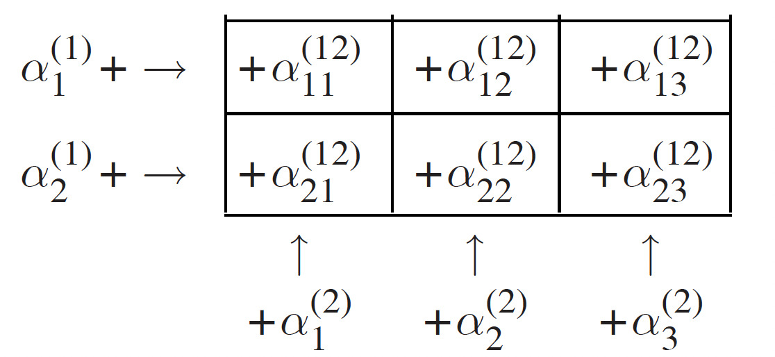
The first risk factor \(\alpha_i^{(1)}\) can be called the row factor. The second risk factor \(\alpha_j^{(2)}\) can be called the column factor. The structural parameters are defined as follows:

\[ \operatorname{Var}\left(\alpha_i^{(1)}\right)=b^{(1)}, \quad \operatorname{Var}\left(\alpha_j^{(2)}\right)=b^{(2)}, \]

\[ \operatorname{Var}\left(\alpha_{i j}^{(12)}\right)=a, \quad \operatorname{Var}\left(\epsilon_{i j t}\right)=s^2 / w_{i j t} . \]

The credibility estimator of \(y_{i j, T_{i j}+1}\) is equal to (Dannenburg, Kaas, and Goovaerts 1996):

\[ \begin{aligned} y_{i j, T_{i j}+1}= & \beta+z_{i j}\left(y_{i j w}-\beta\right)+\left(1-z_{i j}\right) z_i^{(1)}\left(x_{i z w}-\beta\right) \\ & +\left(1-z_{i j}\right) z_j^{(2)}\left(x_{z j w}-\beta\right), \end{aligned} \tag{18} \]

where the credibility factors are

\[ z_{i j}=\frac{a}{a+\sigma^2 / w_{i j \Sigma}}, \quad \text { with } \quad w_{i j \Sigma}=\sum_t w_{i j t}, \tag{19} \]

\[ z_i^{(1)}=\frac{b^{(1)}}{b^{(1)}+a / z_{i \Sigma}}, \quad \text { with } \quad z_{i \Sigma}=\sum_j z_{i j}, \tag{20} \]

\[ z_j^{(2)}=\frac{b^{(2)}}{b^{(2)}+a / z_{\Sigma j}}, \quad \text { with } \quad z_{\Sigma j}=\sum_i z_{i j}. \tag{21} \]

\(x_{i z w}, x_{z j w}\) are the adjusted weighted averages, which can give us a much clearer view on the risk experience with regard to different risk factors,

\[ x_{i z w}=\sum_j \frac{z_{i j}}{z_{i \Sigma}}\left(y_{i j w}-\Xi_j^{(2) *}\right), \tag{22} \]

\[ x_{z j w}=\sum_i \frac{z_{i j}}{z_{\Sigma j}}\left(y_{i j w}-\Xi_i^{(1) *}\right), \tag{23} \]

where

\[ y_{i j w}=\sum_t \frac{w_{i j t}}{w_{i j \Sigma}} y_{i j t} . \]

And \(\Xi_i^{(1) *}, \Xi_j^{(2) *}\) are the row effect and the column effect respectively. They can be found as the solution of the following \(I+J\) linear equations using iterative approach.

\[ \Xi_i^{(1) *}=z_i^{(1)}\left[\sum_j \frac{z_{i j}}{z_{i \Sigma}}\left(y_{i j w}-\Xi_j^{(2) *}\right)-\beta\right], \tag{24} \]

\[ \Xi_j^{(2) *}=z_j^{(2)}\left[\sum_i \frac{z_{i j}}{z_{\Sigma j}}\left(y_{i j w}-\Xi_i^{(1) *}\right)-\beta\right] . \tag{25} \]

In Dannenburg’s approach, the structural parameters β and s² can be estimated by the following equations (Dannenburg, Kaas, and Goovaerts 1996):
\[ \beta=x_{w w w}=\sum_i \sum_j \frac{w_{i j \Sigma}}{w_{\Sigma \Sigma \Sigma}} y_{i j w}, \tag{26} \]

\[ s^{2 \bullet}=\frac{\sum_i \sum_j \sum_t w_{i j t}\left(y_{i j t}-y_{i j w}\right)^2}{\sum_i \sum_j\left(T_{i j}-1\right)_{+}} . \tag{27} \]

To obtain the estimators a, b⁽¹⁾ and b⁽²⁾, Dannenburg, Kaas, and Goovaerts (1996) suggested to solve the following linear equations on moments:

\[ \begin{gathered} E\left[\frac{1}{I} \sum_i\left(\sum_j \frac{w_{i j \Sigma}}{w_{i \Sigma \Sigma}}\left(y_{i j w}-y_{i w w}\right)^2-s^{2 \bullet}(J-1) / w_{i \Sigma \Sigma}\right)\right] \\ \quad=\left(b^{(2)}+a\right)\left(1-\frac{1}{I} \sum_i \sum_j\left(\frac{w_{i j \Sigma}}{w_{i \Sigma \Sigma}}\right)^2\right), \end{gathered} \tag{28} \]

\[ \begin{gathered} E\left[\frac{1}{J} \sum_j\left(\sum_i \frac{w_{i j \Sigma}}{w_{\Sigma j \Sigma}}\left(y_{i j w}-y_{w j w}\right)^2-s^{2 \bullet}(I-1) / w_{\Sigma j \Sigma}\right)\right] \\ \quad=\left(b^{(1)}+a\right)\left(1-\frac{1}{J} \sum_j \sum_i\left(\frac{w_{i j \Sigma}}{w_{\Sigma j \Sigma}}\right)^2\right), \end{gathered} \tag{29} \]

\[ \begin{aligned} E\left[\sum_{i}\right. & \left.\sum_{j} \frac{w_{i j \Sigma}}{w_{\Sigma \Sigma \Sigma}}\left(y_{i j w}-y_{w w w}\right)^{2}-s^{2 \bullet}(I J-1) / w_{\Sigma \Sigma \Sigma}\right] \\ & =b^{(1)}\left(1-\sum_{i}\left(\frac{w_{i \Sigma \Sigma}}{w_{\Sigma \Sigma \Sigma}}\right)^{2}\right) \\ & +b^{(2)}\left(1-\sum_{j}\left(\frac{w_{\Sigma j \Sigma}}{w_{\Sigma \Sigma \Sigma}}\right)^{2}\right) \\ & +a\left(1-\sum_{i} \sum_{j}\left(\frac{w_{i j \Sigma}}{w_{\Sigma \Sigma \Sigma}}\right)\right), \end{aligned} \tag{30} \]

where \(y_{i w w}=\sum_j\left(w_{i j \Sigma} / w_{i \Sigma \Sigma}\right) y_{i j w}\) and \(y_{w j w}= \sum_i\left(w_{i j \Sigma} / w_{\Sigma j \Sigma}\right) y_{i j w}\). To find the “unbiased estimator” of \(a, b^{(1)}\) and \(b^{(2)}\), we can drop the expectation operation of the above linear equations. As we can see, Dannenburg’s estimates are based on the method of moments.

5.2. Empirical studies

Since Dannenburg’s crossed classification model is of the form of linear mixed models, we could make use of the statistical packages that are designed especially for the parameter estimation in linear mixed models. One possibility is SAS. In our simulation studies, the results are obtained from the SAS procedure PROC MIXED. Since the simulation results for the ML and REML estimators are very similar, we only present the results for ML in this paper.

The estimation approaches we consider here are about the same as in Hachemeister’s model, except that the first approach is Dannenburg’s estimation approach. We would also provide two studies which is similar to Section 4. In Study 1, the error terms are simulated from multivariate normal distribution. In Study 2, the error terms are simulated from multivariate lognormal distribution.

5.2.1. Study 1

The simulation study is based on the following choice of parameters:

\[ \begin{aligned} I=12, & J=8, \quad T_{i j}=n=10, \\ b^{(1)}=100, & b^{(2)}=64, \quad a=4, \quad s^{2}=196 . \end{aligned} \]

In this study, the observations are divided into \(I \times J\) cells (96 cells). We randomly select 32 cells first, and these 32 cells have weight \(w_{i j t}=150\); then we select another 32 cells from the rest cells, these 32 cells have weight \(w_{i j t}=10\); the cells left have weight \(w_{i j t}=1.5\). Each sector retains its weight which has been assigned during the first replicate. The error terms \(\epsilon_{i j t} \mathrm{~s}\) are simulated from multivariate normal distribution. The error structure is independent for Table 5 and exchangeable with \(\rho=0.4\) for Table 6.

As for the simulation results, we show the bias and mean square error (MSE) of the Dannenburg and ML approaches for \(\beta, y_{i j, T_{i j}+1}, z_{i j}, z_i^{(1)}, z_j^{(2)}\), \(b^{(1)}, b^{(2)}, a\) and \(s^2\).

We can see from Tables 5 and 6 that a significant advantage has been recorded for the ML approach over Dannenburg’s approach. With regards to the structural parameters, the ML estimators have largely improved the estimation efficiency, especially for the parameters \(a\) and \(b^{(2)}\). As a result, the performance of estimating the credibility factors and \(y_{i j, T_{i j}+1}\) of the ML approach are very impressive. The reason for the poor performance of the Dannenburg estimator is that the level of precision in estimating \(a\) and \(b^{(2)}\) is not enough to produce satisfactory estimates for the credibility factors. From our simulation results, for 500 repetitions, around \(40 \%\) of the estimates of \(a\) are found to be negative, and around \(6 \%\) of the estimates of \(b^{(2)}\) are found to be negative. In contrast, all structural parameters estimated using ML approach fall in an admissible range.

From Table 5, we can see that MSE for \(a\) in Dannenburg’s approach is about 500 times higher than the counterpart in the ML approach. As expected, the ML approach outperforms Dannenburg’s estimation approach in estimating the future exposure \(y\) (relative efficiency around 1000) and the credibility factors (relative efficiency beyond 5000 for \(z_{i j}\) and \(z_j^{(2)}\), relative efficiency beyond 40 for \(z_i^{(1)}\) ). From Table 6, due to the correct assumption made on the error structure, as we can expect that the ML-EX estimator performs the best. The ML-EX estimator maintains the high accuracy level in estimating the structural parameters, especially in estimating a. As a result, the MSE of the credibility factors in the ML-EX method is impressively low.

5.2.2. Study 2

In this study, the setting is similar to Study 1 , except the error terms \(\epsilon_{i j t} \mathrm{~s}\) are simulated from multivariate lognormal distribution. The vector of the error terms has mean shifted to \(\mathbf{0}\), and \(s^2=196\). The error structure is independent in Table 3 and exchangeable with \(\rho=0.4\) in Table 4 . The lognormal distribution has skewness of 2.97 and kurtosis of 25.3 , which substantially departs from normal distribution. The estimators used in this study are the same as in Study 1.

As we explained in Study 1, Dannenburg’s approach fails in providing credible estimates of \(a\) and \(b^{(2)}\). From Table 7, we can observe the large discrepancies in the performance of the estimators for \(y\) and the credibility factors between the ML approach and Dannenburg’s approach. The simulation shows even better results than we have observed in Table 5 in estimating the credibility factors (relative efficiency beyond 10,000 for \(z_{i j}\) and \(z_j^{(2)}\), relative efficiency beyond 100 for \(z_i^{(1)}\) ). From Table 8, the ML-EX outperforms the other methods especially in estimating \(a\) and \(z_i^{(1)}\). Therefore, the simulation results reaffirm that the proposed ML approach can provide us credible estimates even when the distribution of the observation substantially deviates from normality.

6. Concluding remarks

In this paper, we implement the linear mixed model in credibility context and use ML and REML approach to estimate the structural parameters. There are other approaches in estimating the structural parameters in the credibility models. By comparing our approaches with the generalized least square estimation approach proposed by Cossette and Luong (2003) and the GEE approach proposed by Lo, Fung, and Zhu (2006) and Lo, Fung, and Zhu (2007), we demonstrate the merits of our approaches. The former can hardly be extended beyond the Bühlmann model, in which the heteroscedasticity is assumed in the error terms. The latter is hard to apply to classical credibility models when the number of observations with regard to the same contract gets bigger. For instance, if the number of observations for the same contract exceeds 10, the working covariance matrix would be extremely complicated, and the dimension would be very large in the GEE approach. Also the robustness of these two approaches has not been investigated.

Furthermore, from the empirical studies, the time our approach takes is much shorter than the GEE approach. For instance, it takes less than 15 minutes to get the ML and REML estimation results for 500 repetitions in the Hachemeister model using a Pentium 4 3.00 GHz desktop computer with 2.00 GB of RAM; however it takes more than one and a half hours to get the GEE estimates for 500 repetitions. Furthermore, with the aid of software, there are no additional complications when we want to exercise the proposed ML and REML approaches with different assumptions on the error structure.

Moreover, we have investigated the performance of ML and REML methods when the assumptions regarding the error structure and distribution are violated. We can see from the simulation studies, for the situations that the error terms follow normal and non-normal distributions, ML and REML methods maintain satisfactory results. This serves an empirical justification of using the ML and REML approaches when distribution of the observations is unknown.

In this paper, we have only showed the results of the ML approach for brevity. Verbeke and Molenberghs (2000) made the comparison between ML and REML estimation. With regard to the mean squared error of estimating the variance and covariance parameters, neither of the two estimation procedures are universally better than the other. The performance of ML and REML depends on the specification of the underlying model, and possibly on the true value of the variance and covariance parameters. However, when the rank of design matrix \(\mathbf{X}_i\) is less than 4 , the ML estimator of the residual \(\sigma^2\) generally outperforms the REML estimator, but the opposite is true when the rank of \(\mathbf{X}_i\) gets larger. Generally speaking, we can expect the difference between ML and REML estimator increases when the rank of \(\mathbf{X}_i\) increases. In our simulation studies, since the rank of \(\mathbf{X}_i\) is not large, neither the ML approach or the REML approach performs universally better than the other in both Dannenburg’s model and Hachemeister model.