The Bornhuetter-Ferguson Principle

undefined

1. Introduction

During the last decades, actuaries have proposed a large variety of methods of loss reserving based on run-off triangles. In each of these methods, it is assumed that all claims are settled within a fixed number of development years and that the development of incremental or cumulative losses from the same number of accident years is known up to the present calendar year such that the losses can be represented in a run-off triangle.

The most venerable and most famous of these methods are certainly the chain-ladder method and the Bornhuetter-Ferguson method. It appears that the basic idea of the chain-ladder method was already known to Tarbell (1934), while the Bornhuetter-Ferguson method was first described almost 40 years later in the paper by Bornhuetter and Ferguson (1972).

At the first glance, the methods have very little in common:

• The chain-ladder method proposes predictors of the ultimate (cumulative) losses and every predictor is obtained sequentially by multiplying the current (cumulative) loss by the chain-ladder factors which are certain development factors (or link ratios) obtained from the run-off triangle.

• The Bornhuetter-Ferguson method proposes predictors of the outstanding losses and every predictor is obtained by multiplying an estimator of the expected ultimate (cumulative) loss by an estimator of the percentage of the outstanding loss with respect to the ultimate one.

The fact that these methods aim at different target quantities can be neglected since predictors of ultimate losses can be converted into predictors of outstanding losses, and vice versa. However, a crucial difference lies in the fact that the chain-ladder method proceeds from current losses while the Bornhuetter-Ferguson method is based on the expected ultimate losses, and this difference is connected with the sources of information which are taken into account:

• The chain-ladder method relies completely on the data contained in the run-off triangle.

• The Bornhuetter-Ferguson method restricts the use of the run-off triangle to the estimation of the percentage of the outstanding loss and uses the product of the earned premium and an expected loss ratio to estimate the expected ultimate loss.

The aim of this paper is to show that, in spite of their different appearances, the chain-ladder method and the Bornhuetter-Ferguson method, as well as many other methods of loss reserving, have indeed very much in common.

The striking point with the Bornhuetter-Ferguson method is the multiplicative structure of the predictors of the outstanding losses. In the original version of the method, each of the two factors has the particular meaning mentioned before. This interpretation may be dropped. If it is dropped, then we obtain predictors each of which is the product of some estimator of the ultimate loss and some estimator of the percentage of outstanding losses, and we are free to choose these estimators as we like.

We thus arrive at a general class of predictors of outstanding losses, and hence at a corresponding class of predictors of ultimate losses.^[1] The predictors of this class will be referred to as predictors of the extended Bornhuetter-Ferguson method. It will be shown that the chain-ladder predictors belong to this class and that the predictors of many other methods of loss reserving belong to this class as well.

Since the prediction of outstanding or ultimate losses is a statistical problem, it is most helpful to formulate all methods (which in many cases were originally designed as deterministic algorithms) in a statistical setting. This means that all losses are interpreted as random variables which are either observable or not. In particular, the data represented in a run-off triangle are interpreted as realizations of observable losses and the outstanding or ultimate losses are non-observable (except for the initial accident year).

Once the statistical setting is accepted, the fundamental notion of a development pattern can be introduced. Although the notion of a development pattern is more or less present in many publications on loss reserving, its force with regard to the comparison of methods has been made evident only recently; see Radtke and Schmidt (2004) and Schmidt (2006).

Using the notion of a development pattern, we will show that the extended Bornhuetter-Ferguson method is not just a particular one among various methods of loss reserving but is a general one which contains many other methods as special cases and leads to the Bornhuetter-Ferguson principle, which consists of the simultaneous application of several versions of the extended Bornhuetter-Ferguson method to a given run-off triangle.

This paper extends the discussion of the extended Bornhuetter-Ferguson method which was started in some of the contributions in Radtke and Schmidt (2004) and was continued in Schmidt (2006; Section 4). The extension consists of

• the inclusion of development patterns which differ from the classical ones,

• a general discussion of the estimation of development patterns, and

• the embedding of quite recent methods of loss reserving into the extended Bornhuetter-Ferguson method.

In particular, we take into account the contributions of Mack (2006) and Panning (2006) in response to the CAS 2006 Reserves Call Paper Program.

This paper is organized as follows:

In Section 2, we introduce the general modeling of loss development data by a family of random variables representing the incremental or cumulative losses and the representation of the observable incremental or cumulative losses by a run-off triangle.

In Section 3, we introduce and study the central notion of a development pattern which turns out to be a powerful and unifying concept for the interpretation and comparison of several methods of loss reserving based on run-off triangles. We show that the notion of a development pattern can be expressed in several different but equivalent ways and that a development pattern can also be obtained on the basis of volume measures.

In Section 4, we study the problem of estimating the parameters of a development pattern.

In Section 5, we present the extended Bornhuetter-Ferguson method in its predictive form for the ultimate (cumulative) losses and we show that many other methods of loss reserving can be interpreted as special cases. This section is the central part of the present paper. The results of this section are summarized in a table which indicates that certain combinations of estimators of the development pattern and of the expected ultimate losses yield new methods of loss reserving which have not yet been considered in the literature.

In Section 6, we illustrate possible applications of the Bornhuetter-Ferguson principle by a numerical example. For a given run-off triangle, we use a variety of versions of the extended Bornhuetter-Ferguson method to compute predictors of the first year reserve and the total reserve. The realizations of these predictors are visualized in a two-dimensional plot which, when combined with actuarial judgment, may be used to determine best predictors and ranges; in addition, they may be used to compare the portfolio under consideration with a market portfolio or to check whether premiums are adequate or not.

In Section 7, we present proofs of two nonevident results used in Section 5.

2. Run-off triangles

We consider a portfolio of risks and we assume that each claim of the portfolio is settled either in the accident year or in the following n development years. The portfolio may be modeled either by incremental losses or by cumulative losses.

2.1. Incremental losses

To model a portfolio by incremental losses, we consider a family of random variables $\left\{Z_{i, k}\right\}_{i, k \in\{0,1, \ldots, n\}}$ and we interpret the random variable $Z_{i, k}$ as the loss of accident year $i$ which is settled with a delay of $k$ years and hence in development year $k$ and in calendar year $i+k$. We refer to $Z_{i, k}$ as the incremental loss of accident year $i$ and development year $k$.

We assume that the incremental losses $Z_{i, k}$ are observable for calendar years $i+k \leq n$ and that they are non-observable for calendar years $i+k \geq n+1$. The observable incremental losses are represented by the following run-off triangle:

The problem is to predict the non-observable incremental losses.

2.2. Cumulative losses

To model a portfolio by incremental losses, we consider a family of random variables $\left\{S_{i, k}\right\}_{i, k \in\{0,1, \ldots, n\}}$ and we interpret the random variable $S_{i, k}$ as the loss of accident year $i$ which is settled with a delay of at most $k$ years and hence not later than in development year $k$. We refer to $S_{i, k}$ as the cumulative loss of accident year $i$ and development year $k$, to $S_{i, n-i}$ as a cumulative loss of the present calendar year $n$ or as a current (cumulative) loss, and to $S_{i, n}$ as an ultimate (cumulative) loss.

We assume that the cumulative losses $S_{i, k}$ are observable for calendar years $i+k \leq n$ and that they are non-observable for calendar years $i+k \geq n+1$. The observable cumulative losses are represented by the following run-off triangle:

The problem is to predict the non-observable incremental losses.

2.3. Remarks

Of course, modeling a portfolio by incremental losses is equivalent to modeling a portfolio by cumulative losses:

• The cumulative losses are obtained from the incremental losses by letting $$S_{i, k}:=\sum_{l=0}^k Z_{i, l} .$$ Then the non-observable cumulative losses satisfy $$S_{i, k}=S_{i, n-i}+\sum_{l=n-i+1}^k Z_{i, l} .$$

• The incremental losses are obtained from the cumulative losses by letting

$$Z_{i, k}:=\left\{\begin{array}{ll} S_{i, 0} & \text { if } \quad k=0 \\ S_{i, k}-S_{i, k-1} & \text { else } \end{array} .\right.$$

In the sequel we shall switch between incremental and cumulative losses as necessary.

Correspondingly, prediction of non-observable incremental losses is equivalent to prediction of non-observable cumulative losses:

• If $\left\{\hat{Z}_{i, k}\right\}_{i, k \in\{0,1, \ldots, n\}, i+k \geq n+1}$ is a family of predictors of the non-observable incremental losses, then a family of predictors of the nonobservable cumulative losses is obtained by letting

$$\hat{S}_{i, k}:=S_{i, n-i}+\sum_{l=n-i+1}^k \hat{Z}_{i, l} .$$

• If $\left\{\hat{S}_{i, k}\right\}_{i, k \in\{0,1, \ldots, n\}, i+k \geq n+1}$ is a family of predictors of the non-observable cumulative losses, then a family of predictors of the non-observable incremental losses is obtained by letting

$$\hat{Z}_{i, k}:=\left\{\begin{array}{ll} \hat{S}_{i, n-i+1}-S_{i, n-i} & \text { if } k=n-i+1 \\ \hat{S}_{i, k}-\hat{S}_{i, k-1} & \text { else } \end{array} .\right.$$

For the ease of notation and to avoid the distinction of cases as in the previous definition, we shall also refer to $Z_{i, n-i}$ and $S_{i, n-i}$ as predictors of $Z_{i, n-i}$ and $S_{i, n-i}$, although these random variables are, of course, observable.

The enumeration of accident years and development years starting with 0 instead of 1 is widely but not yet generally accepted; see Stanard (1985), Taylor (2000), Radtke and Schmidt (2004), Panning (2006), and the publications of the present authors. It is useful for several reasons:

• For losses which are settled within the accident year, the delay of settlement is 0. It is therefore natural to start the enumeration of development years with 0.

• Using the enumeration of development years also for accident years implies that the incremental or cumulative loss of accident year $i$ and development year $k$ is observable if and only if $i+k \leq n$. In particular, the current losses $S_{i, n-i}$ are those of the present calendar year $n$ and are crucial in most methods of loss reserving.

After all, the notation used here simplifies mathematical formulas.

3. Development patterns

The use of run-off triangles in loss reserving can be justified only if it is assumed that the development of the losses of every accident year follows a development pattern which is common to all accident years. This vague idea of a development pattern can be formalized in various ways.

In the present section we consider three classical development patterns, which are formally distinct but nevertheless similar and can easily be converted into each other, and we also introduce alternative development patterns. The variety of development patterns is nevertheless needed since each of these development patterns occurs as a natural primitive model for some of the methods of loss reserving to be discussed in Section 5 or as a part of certain more sophisticated models; see Schmidt (2006).

The assumption of an underlying development pattern can be viewed as a primitive stochastic model and provides the key to the comparison of various methods of loss reserving.

3.1. Incremental quotas

A vector $\boldsymbol{\vartheta}=\left(\vartheta_0, \vartheta_1, \ldots, \vartheta_n\right)$ of parameters (with $\sum_{l=0}^n \vartheta_l=1$ ) is said to be a development pattern for incremental quotas if the identity

$$\vartheta_k=\frac{E\left[Z_{i, k}\right]}{E\left[S_{i, n}\right]}$$

holds for all $k \in\{0,1, \ldots, n\}$ and for all $i \in\{0,1$, $\ldots, n\}$.

Thus, a development pattern for incremental quotas exists if, and only if, for every development year $k \in\{0,1, \ldots, n\}$ the individual incremental quotas

$$\vartheta_{i, k}:=\frac{E\left[Z_{i, k}\right]}{E\left[S_{i, n}\right]}$$

are identical for all accident years.

In the case of a run-off triangle for paid losses or claim counts it is usually reasonable to assume in addition that $\vartheta_k>0$ holds for all $k \in \{0,1, \ldots, n\}$. In the case of incurred losses, however, this additional assumption may be inappropriate since, due to conservative loss reserving, the expected incremental losses of development years $k \in\{1, \ldots, n\}$ may be negative.

3.2. Cumulative quotas

A vector $\gamma=\left(\gamma_0, \gamma_1, \ldots, \gamma_n\right)$ of parameters (with $\gamma_n=1$ ) is said to be a development pattern for cumulative quotas if the identity

$$\gamma_{k}=\frac{E\left[S_{i, k}\right]}{E\left[S_{i, n}\right]}$$

holds for all $k \in\{0,1, \ldots, n\}$ and for all $i \in\{0,1$, $\ldots, n\}$.

Thus, a development pattern for cumulative quotas exists if, and only if, for every development year $k \in\{0,1, \ldots, n\}$ the individual cumulative quotas

$$\gamma_{i, k}:=\frac{E\left[S_{i, k}\right]}{E\left[S_{i, n}\right]}$$

are identical for all accident years.

In the case of a run-off triangle for paid losses or claim counts, it is usually reasonable to assume in addition that $0<\gamma_0<\gamma_1<\cdots<\gamma_n$.

The development patterns for cumulative quotas and for incremental quotas can be converted into each other:

• If γ is a development pattern for cumulative quotas, then a development pattern ϑ for incremental quotas is obtained by letting

  $$\vartheta_{k}:=\left\{\begin{array}{ll} \gamma_{0} & \text { if } k=0 \\ \gamma_{k}-\gamma_{k-1} & \text { else } \end{array} .\right.$$

• If ϑ is a development pattern for incremental quotas, then a development pattern γ for cumulative quotas is obtained by letting

  $$\gamma_{k}:=\sum_{l=0}^{k} \vartheta_{l} .$$

Furthermore, the condition $0<\gamma_0<\gamma_1<\cdots<\gamma_n$ is fulfilled if, and only if, $\vartheta_k>0$ holds for all $k \in\{0,1, \ldots, n\}$.

3.3. Factors

A vector $\varphi=\left(\varphi_1, \ldots, \varphi_n\right)$ of parameters is said to be a development pattern for factors if the identity

$$\varphi_{k}=\frac{E\left[S_{i, k}\right]}{E\left[S_{i, k-1}\right]}$$

holds for all $k \in\{1, \ldots, n\}$ and for all $i \in\{0,1$, $\ldots, n\}$.

Thus, a development pattern for factors exists if, and only if, for every development year $k \in \{1 \ldots n\}$ the individual factors

$$\varphi_{i, k}:=\frac{E\left[S_{i, k}\right]}{E\left[S_{i, k-1}\right]}$$

are identical for all accident years.

In the case of a run-off triangle for paid losses or claim counts, it is usually reasonable to assume in addition that $\varphi_k>1$ holds for all $k \in \{1, \ldots, n\}$.

The development patterns for factors and for cumulative quotas can be converted into each other:

• If φ is a development pattern for factors, then a development pattern γ for cumulative quotas is obtained by letting

  $$\gamma_{k}:=\prod_{l=k+1}^{n} \frac{1}{\varphi_{l}} .$$

• If γ is a development pattern for cumulative quotas, then a development pattern φ for factors is obtained by letting

  $$\varphi_{k}:=\frac{\gamma_{k}}{\gamma_{k-1}},$$

Furthermore, $\varphi_k>1$ holds for all $k \in\{1, \ldots, n\}$ if, and only if, the condition $\gamma_0<\gamma_1<\cdots<\gamma_n$ is fulfilled.

Combining the previous result and that of the preceding subsection, it is evident that also the development patterns for factors and for incremental quotas can be converted into each other.

3.4. Incremental ratios

The classical development patterns considered before are quite familiar and have been shown to be equivalent.

An alternative development pattern can be distilled from the paper by Panning (2006) which was written in response to the CAS 2006 Reserves Call Paper Program:

A vector $\boldsymbol{\beta}=\left(\beta_0, \beta_1, \ldots, \beta_n\right)$ of parameters (with $\beta_0=1$ ) is said to be a development pattern for incremental ratios if the identity

$$\beta_{k}=\frac{E\left[Z_{i, k}\right]}{E\left[Z_{i, 0}\right]}$$

holds for all k ∈ {0, 1, . . . , n} and for all i ∈ {0, 1, . . . , n}.

Thus, a development pattern for incremental ratios exists if, and only if, for every development year k ∈ {0, 1, . . . , n} the individual incremental ratios

$$\beta_{i, k}:=\frac{E\left[Z_{i, k}\right]}{E\left[Z_{i, 0}\right]}$$

are identical for all accident years.

In the case of a run-off triangle for paid losses or claim counts it is usually reasonable to assume in addition that $\beta_k>0$ holds for all $k \in \{0,1, \ldots, n\}$.

The development patterns for incremental ratios and for incremental quotas can be converted into each other:

• If β is a development pattern for incremental ratios, then a development pattern ϑ for incremental quotas is obtained by letting

  $$\vartheta_{k}:=\frac{\beta_{k}}{\sum_{l=0}^{n} \beta_{l}}.$$

• If ϑ is a development pattern for incremental quotas, then a development pattern β for incremental ratios is obtained by letting

  $$\beta_{k}:=\frac{\vartheta_{k}}{\vartheta_{0}} .$$

Moreover, the development patterns for incremental ratios and for cumulative quotas can be converted into each other as well:

• If β is a development pattern for incremental ratios, then a development pattern γ for cumulative quotas is obtained by letting

  $$\gamma_{k}:=\frac{\sum_{l=0}^{k} \beta_{l}}{\sum_{l=0}^{n} \beta_{l}}.$$

• If γ is a development pattern for cumulative quotas, then a development pattern β for incremental ratios is obtained by letting

  $$\beta_{k}:=\left\{\begin{array}{ll} 1 & \text { if } k=0 \\ \frac{\gamma_{k}-\gamma_{k-1}}{\gamma_{0}} & \text { else } \end{array} .\right.$$

Furthermore, $\beta_k>0$ holds for all $k \in\{0,1, \ldots, n\}$ if and only if $\vartheta_k>0$ holds for all $k \in\{0,1, \ldots, n\}$, and this is the case if and only if $0<\gamma_0<\gamma_1< \cdots<\gamma_n$.

3.5. Incremental loss ratios

The development patterns considered so far are completely determined by expected incremental or cumulative losses. However, if a vector $\pi=$ ( $\pi_0, \pi_1, \ldots, \pi_n$ ) of known volume measures (like premiums or the number of contracts) is given, then another development pattern can be defined which also depends on the volume measure $\pi$.

A vector $\zeta(\pi)=\left(\zeta_0(\pi), \zeta_1(\pi), \ldots, \zeta_n(\pi)\right)$ of pa-rameters is said to be a development pattern for incremental loss ratios if the identity

$$\zeta_{k}(\pi)=E\left[\frac{Z_{i, k}}{\pi_{i}}\right]$$

holds for all k ∈ {0, 1, . . . , n} and for all i ∈ {0, 1, . . . , n}.

Thus, a development pattern for incremental loss ratios exists if, and only if, for every development year k ∈ {0, 1, . . . , n} the individual incremental loss ratios

$$\zeta_{i, k}(\pi):=E\left[\frac{Z_{i, k}}{\pi_{i}}\right]$$

are identical for all accident years.

In the case of a run-off triangle for paid losses or claim counts it is usually reasonable to assume in addition that $\zeta_k(\pi)>0$ holds for all $k \in \{0,1, \ldots, n\}$.

If ζ(π) is a development pattern for incremental loss ratios, then

• a development pattern ϑ(π) for incremental quotas is obtained by letting

  $$\vartheta_{k}(\pi):=\frac{\zeta_{k}(\pi)}{\sum_{l=0}^{n} \zeta_{l}(\pi)}$$

  and

• a development pattern γ(π) for cumulative quotas is obtained by letting

  $$\gamma_{k}(\boldsymbol{\pi}):=\frac{\sum_{l=0}^{k} \zeta_{l}(\boldsymbol{\pi})}{\sum_{l=0}^{n} \zeta_{l}(\boldsymbol{\pi})}$$

These definitions are entirely analogous to those used in the case of a development pattern for incremental ratios.

3.6. Remarks

In the case of a run-off triangle for paid losses or claim counts, the intuitive interpretation of the development patterns of incremental or cumulative quotas would be their interpretation as incremental or cumulative probabilities. This interpretation is helpful, but it is not quite correct since the parameters of these development patterns are defined in terms of quotients of expectations instead of expectations of quotients; as it is well-known, these quantities are in general distinct.

One may thus argue that the definitions of development patterns are inconvenient since they do not exactly correspond to intuition. The development patterns defined in terms of quotients of expectations are nevertheless reasonable since they are all equivalent in the sense that they can be converted into each other (which would be impossible for certain development patterns defined in terms of expectations of quotients). Due to this equivalence, the development patterns presented here provide a powerful and unifying concept for the interpretation and comparison of several methods of loss reserving.

Quite generally, alternative development patterns can be derived from the classical ones by interchanging the roles of incremental and cumulative losses and/or the roles of the initial and the ultimate development year. In this sense, the development pattern for incremental ratios corresponds to the development pattern for cumulative quotas.

4. Estimation of development patterns

For each of the methods of loss reserving to be discussed in Section 5, the predictors of the ultimate losses can be justified by the assumption that a development pattern exists. This is due to the fact that, in either case, the predictors can be expressed in terms of certain estimators of the parameters of the development pattern for cumulative quotas.

Quite generally, estimation of the development pattern can be based on one or both of the following different sources of information:

• Internal information: This is any information which is completely contained in the run-off triangle of the portfolio under consideration.

• External information: This is any information which is completely independent of the run-off triangle of the portfolio under consideration. External information could be obtained, e.g., from market statistics or from other portfolios which are judged to be similar to the given one; also, volume measures (like premiums or the number of contracts) for the given portfolio present external information since they are not contained in the run-off triangle.

Of course, these different sources of information may also be combined, in which case estimation is based on mixed information.

It is possible to develop a general theory on the estimation of the parameters of a development pattern, but this would exceed the scope of the present paper. Instead, we shall confine ourselves to the presentation of the three types of estimators which will be needed in Section 5. The first two of these estimators are entirely based on internal information while the third one is based on mixed information. Nevertheless, the similarity of these three types of estimators indicates a general principle of estimation which can be applied to any development pattern.

The estimators presented below are based on the development patterns for factors, incremental ratios, and incremental loss ratios, respectively. Since each of these development patterns can be converted into a development pattern for cumulative quotas, as shown in Section 3, the same conversion formulas will be used to convert these estimators into estimators of the parameters of the corresponding development pattern for cumulative quotas.

4.1. Estimation from empirical individual factors

At the first glance, there is little hope to estimate the parameters of the development patterns for incremental or cumulative quotas since the only obvious estimators of $\vartheta_k$ and $\gamma_k$ are the empirical individual incremental quotas $Z_{0, k} / S_{0, n}$ and the empirical individual cumulative quotas $S_{0, k} / S_{0, n}$, respectively. Fortunately, the situation is quite different for the development pattern for factors:

Assume that $\varphi=\left(\varphi_1, \ldots, \varphi_n\right)$ is a development pattern for factors. Then, for every development year $k \in\{1, \ldots, n\}$, each of the empirical individual factors or link ratios

$$\hat{\varphi}_{i, k}:=\frac{S_{i, k}}{S_{i, k-1}}$$

with $i \in\{0,1, \ldots, n-k\}$ is a reasonable estimator of $\varphi_k$, and this is also true for every weighted mean

$$\hat{\varphi}_k:=\sum_{j=0}^{n-k} W_{j, k} \hat{\varphi}_{j, k}$$

with random variables (or constants) satisfying $\sum_{j=0}^{n-k} W_{j, k}=1$. The most prominent estimator of this large family is the chain-ladder factor

$$\hat{\varphi}_{k}^{\mathrm{CL}}:=\frac{\sum_{j=0}^{n-k} S_{j, k}}{\sum_{j=0}^{n-k} S_{j, k-1}}=\sum_{j=0}^{n-k} \frac{S_{j, k-1}}{\sum_{h=0}^{n-k} S_{h, k-1}} \hat{\varphi}_{j, k},$$

which is used in the chain-ladder method. We denote by

$$\hat{\varphi}^{\mathrm{CL}}:=\left(\hat{\varphi}_{1}^{\mathrm{CL}}, \ldots, \hat{\varphi}_{n}^{\mathrm{CL}}\right)$$

the random vector consisting of all chain-ladder factors.

Due to the correspondence between the development patterns for factors and for cumulative quotas, it is clear that in the same way estimators of factors can be converted into estimators of cumulative quotas. In particular, the chain-ladder quotas

$$\hat{\gamma}_{k}^{\mathrm{CL}}:=\prod_{l=k+1}^{n} \frac{1}{\hat{\varphi}_{l}^{\mathrm{CL}}}$$

serve as estimators of the cumulative quotas

$$\gamma_{k}:=\prod_{l=k+1}^{n} \frac{1}{\varphi_{l}} .$$

We denote by

$$\hat{\gamma}^{\mathrm{CL}}:=\left(\hat{\gamma}_{0}^{\mathrm{CL}}, \hat{\gamma}_{1}^{\mathrm{CL}}, \ldots, \hat{\gamma}_{n}^{\mathrm{CL}}\right)$$

the random vector consisting of all chain-ladder quotas.

We remark that the chain-ladder quotas are entirely based on internal information.

4.2. Estimation from empirical individual incremental ratios

Assume that $\boldsymbol{\beta}=\left(\beta_0, \beta_1, \ldots, \beta_n\right)$ is a development pattern for incremental ratios. Then, for every development year $k \in\{0,1, \ldots, n\}$, each of the empirical individual incremental ratios

$$\hat{\beta}_{i, k}:=\frac{Z_{i, k}}{Z_{i, 0}}$$

with i ∈ {0, 1, . . . , n − k} is a reasonable estimator of $\beta_{k}$, and this is also true for every weighted mean

$$\hat{\beta}_{k}:=\sum_{j=0}^{n-k} W_{j, k} \hat{\beta}_{j, k}$$

with random variables (or constants) satisfying $\sum_{j=0}^{n-k} W_{j, k}=1$. An example of this large family is the Panning ratio

$$\hat{\beta}_{k}^{\text {Panning}}:=\frac{\sum_{j=0}^{n-k} Z_{j, k} Z_{j, 0}}{\sum_{j=0}^{n-k} Z_{j, 0}^{2}}=\sum_{j=0}^{n-k} \frac{Z_{j, 0}^{2}}{\sum_{h=0}^{n-k} Z_{h, 0}^{2}} \hat{\beta}_{j, k}$$

which is used in Panning’s method. We denote by

$$\hat{\boldsymbol{\beta}}^{\text {Panning}}:=\left(\hat{\beta}_{0}^{\text {Panning}}, \hat{\beta}_{1}^{\text {Panning}}, \ldots, \hat{\beta}_{n}^{\text {Panning}}\right)$$

the random vector consisting of all Panning ratios.

Due to the correspondence between the development patterns for incremental ratios and for cumulative quotas, it is clear that in the same way estimators of incremental ratios can be converted into estimators of cumulative quotas. In particular, the Panning quotas

$$\hat{\gamma}_{k}^{\text {Panning}}:=\frac{\sum_{l=0}^{k} \hat{\beta}_{l}^{\text {Panning}}}{\sum_{l=0}^{n} \hat{\beta}_{l}^{\text {Panning}}}$$

serve as estimators of the cumulative quotas

$$\gamma_{k}:=\frac{\sum_{l=0}^{k} \beta_{l}}{\sum_{l=0}^{n} \beta_{l}}$$

We denote by

$$\hat{\gamma}^{\text {Panning}}:=\left(\hat{\gamma}_{0}^{\text {Panning}}, \hat{\gamma}_{1}^{\text {Panning}}, \ldots, \hat{\gamma}_{n}^{\text {Panning}}\right)$$

the random vector consisting of all Panning quotas.

We remark that the Panning quotas are entirely based on internal information.

4.3. Estimation from empirical individual incremental loss ratios

Assume that $\boldsymbol{\pi}=\left(\pi_0, \pi_1, \ldots, \pi_n\right)$ is a vector of known volume measures and that $\zeta(\pi)=\left(\zeta_0(\pi)\right.$, $\left.\zeta_1(\pi), \ldots, \zeta_n(\pi)\right)$ is a development pattern for loss ratios. Then, for every development year $k \in\{0,1, \ldots, n\}$, each of the empirical individual incremental loss ratios

$$\hat{\zeta}_{i, k}(\pi):=\frac{Z_{i, k}}{\pi_{i}}$$

with $i \in\{0,1, \ldots, n-k\}$ is a reasonable estimator of $\zeta_k(\pi)$, and this is also true for every weighted mean

$$\hat{\zeta}_k(\boldsymbol{\pi}):=\sum_{j=0}^{n-k} W_{j, k} \hat{\zeta}_{j, k}(\boldsymbol{\pi})$$

with random variables (or constants) satisfying $\sum_{j=0}^{n-k} W_{j, k}=1$. The most prominent estimator of this large family is the additive loss ratio

$$\hat{\zeta}_{k}^{\mathrm{AD}}(\boldsymbol{\pi}):=\frac{\sum_{j=0}^{n-k} Z_{j, k}}{\sum_{j=0}^{n-k} \pi_{j}}=\sum_{j=0}^{n-k} \frac{\pi_{j}}{\sum_{h=0}^{n-k} \pi_{h}} \hat{\zeta}_{j, k}(\boldsymbol{\pi}),$$

which is used in the additive method. We denote by

$$\hat{\zeta}^{\mathrm{AD}}(\pi):=\left(\hat{\zeta}_{0}^{\mathrm{AD}}(\pi), \hat{\zeta}_{1}^{\mathrm{AD}}(\pi), \ldots, \hat{\zeta}_{n}^{\mathrm{AD}}(\pi)\right)$$

the random vector consisting of all additive loss ratios.

In view of the transformation of a development pattern for incremental loss ratios into a develpment pattern for cumulative quotas, it is clear that in the same way estimators of incremental loss ratios can be converted into estimators of cumulative quotas. In particular, the additive quotas

$$\hat{\gamma}_{k}^{\mathrm{AD}}(\pi):=\frac{\sum_{l=0}^{k} \hat{\zeta}_{l}^{\mathrm{AD}}(\pi)}{\sum_{l=0}^{n} \hat{\zeta}_{l}^{\mathrm{AD}}(\pi)}$$

serve as estimators of the cumulative quotas

$$\gamma_{k}(\pi):=\frac{\sum_{l=0}^{k} \zeta_{l}(\pi)}{\sum_{l=0}^{n} \zeta_{l}(\pi)}.$$

We denote by

$$\hat{\gamma}^{\mathrm{AD}}(\pi):=\left(\hat{\gamma}_{0}^{\mathrm{AD}}(\pi), \hat{\gamma}_{1}^{\mathrm{AD}}(\pi), \ldots, \hat{\gamma}_{n}^{\mathrm{AD}}(\pi)\right)$$

the random vector consisting of all additive quotas.

We remark that the additive quotas are based on mixed information, since they involve the internal information provided by the run-off triangle and the external information provided by the volume measure.

4.4. Remarks

The use of weighted means in estimating the parameters of a development pattern can be justified in a linear model with uncorrelated dependent variables and suitably chosen variances. For example,

• the chain-ladder factors can be justified in the chain-ladder model of Mack and Schnaus [see Mack (1994), Schmidt and Schnaus (1996), Radtke and Schmidt (2004), and Schmidt (2006)],

• the Panning ratios can be justified in the model of Panning (2006), and

• the additive loss ratios can be justified in the linear model of Mack [see Mack (1991), Radtke and Schmidt (2004), and Schmidt (2006)].

Each of these models is a linear model with a particular assumption on the variances and the afore-mentioned estimators have the Gauss-Markov property. If, however, in any of these models the assumption on the variances would be changed, then the Gauss-Markov estimators of the parameters would be weighted means which are distinct from the chain-ladder factors, the Panning ratios, or the additive loss ratios, respectively.

5. Prediction of ultimate losses

The present section provides a unifying presentation of the most important methods of loss reserving. The starting point is an extension of the Bornhuetter-Ferguson method which is closely related to the notion of a development pattern for cumulative quotas and turns out to be a unifying principle under which various other methods of loss reserving can be subsumed.

5.1. Extended Bornhuetter-Ferguson method

The extended Bornhuetter-Ferguson method is based on the assumption that there exist vectors $\boldsymbol{\alpha}=\left(\alpha_0, \alpha_1, \ldots, \alpha_n\right)$ and $\gamma=\left(\gamma_0, \gamma_1, \ldots, \gamma_n\right)$ of parameters (with $\gamma_n=1$ ) such that the identity

$$E\left[S_{i, k}\right]=\gamma_{k} \alpha_{i}$$

holds for all k ∈ {0, 1, . . . , n} and for all i ∈ {0, 1, . . . , n}. Then we have

$$E\left[S_{i, n}\right]=\alpha_{i}$$

and hence

$$\gamma_{k}=\frac{E\left[S_{i, k}\right]}{E\left[S_{i, n}\right]},$$

which means that γ is a development pattern for cumulative quotas.

The extended Bornhuetter-Ferguson method is also based on the additional assumption that a vector

$$\hat{\gamma}=\left(\hat{\gamma}_{0}, \hat{\gamma}_{1}, \ldots, \hat{\gamma}_{n}\right)$$

of prior estimators of the cumulative quotas with $\hat{\gamma}_n=1$ and a vector

$$\hat{\boldsymbol{\alpha}}=\left(\hat{\alpha}_{0}, \hat{\alpha}_{1}, \ldots, \hat{\alpha}_{n}\right)$$

of prior estimators of the expected ultimate losses are given.^[2] As already indicated in Section 4, the prior estimators of the cumulative quotas can be obtained from internal, external, or mixed information. This is, of course, also true for the prior estimators of the expected ultimate losses.

The Bornhuetter-Ferguson predictors of the cumulative losses $S_{i, k}$ with i + k ≥ n are defined as

$$\hat{S}_{i, k}^{\mathrm{BF}}(\hat{\gamma}, \hat{\boldsymbol{\alpha}}):=S_{i, n-i}+\left(\hat{\gamma}_{k}-\hat{\gamma}_{n-i}\right) \hat{\alpha}_{i} .$$

The definition of the Bornhuetter-Ferguson predictors reminds us of the identity

$$E\left[S_{i, k}\right]=E\left[S_{i, n-i}\right]+\left(\gamma_{k}-\gamma_{n-i}\right) \alpha_{i}$$

which is a consequence of the model assumption. We denote by

$$\hat{\mathbf{S}}^{\mathrm{BF}}(\hat{\gamma}, \hat{\boldsymbol{\alpha}}):=\left(\hat{S}_{i, k}^{\mathrm{BF}}(\hat{\gamma}, \hat{\boldsymbol{\alpha}})\right)_{i, k \in\{0,1, \ldots, n\}, i+k \geq n}$$

the triangle of all Bornhuetter-Ferguson predictors.

Taking the difference between the Bornhuetter-Ferguson predictors and the current losses yields

$$\hat{S}_{i, k}^{\mathrm{BF}}(\hat{\gamma}, \hat{\boldsymbol{\alpha}})-S_{i, n-i}=\left(\hat{\gamma}_{k}-\hat{\gamma}_{n-i}\right) \hat{\alpha}_{i} .$$

In the case k = n this yields

$$\hat{S}_{i, n}^{\mathrm{BF}}(\hat{\gamma}, \hat{\boldsymbol{\alpha}})-S_{i, n-i}=\left(1-\hat{\gamma}_{n-i}\right) \hat{\alpha}_{i},$$

which is a predictor of the reserve $S_{i, n}-S_{i, n-i}$ of accident year $i$ and has the shape of the reserve predictors proposed by Bornhuetter and Ferguson (1972). However, in the original form of the Bornhuetter-Ferguson method it is assumed that the prior estimators of the expected ultimate losses are based on premiums and expected loss ratios while those of the development pattern are obtained from the run-off triangle. Both assumptions are dropped in the extended Bornhuetter-Ferguson method, and this is the key to arranging various methods of loss reserving, which at the first glance have little in common, under a common umbrella.

5.2. Iterated Bornhuetter-Ferguson method

In the case where the current losses are judged to be reliable, it may be desirable to modify the Bornhuetter-Ferguson predictors in order to strengthen the weight of the current losses and to reduce that of the prior estimators of the expected ultimate losses. This goal can be achieved by iteration.

For example, if on the right-hand side of the formula defining the Bornhuetter-Ferguson predictors the prior estimators $\hat{\alpha}_i$ are replaced by the Bornhuetter-Ferguson predictors $\hat{S}_{i, n}^{\mathrm{BF}}$, then the resulting predictors of the cumulative losses $S_{i, k}$ with $i+k \geq n$ are the Benktander-Hovinen predictors^[3]

$$\hat{S}_{i, k}^{\mathrm{BH}}(\hat{\gamma}, \hat{\boldsymbol{\alpha}}):=S_{i, n-i}+\left(\hat{\gamma}_{k}-\hat{\gamma}_{n-i}\right) \hat{S}_{i, n}^{\mathrm{BF}}(\hat{\gamma}, \hat{\boldsymbol{\alpha}}),$$

which, in the case $\hat{\gamma}_0<\hat{\gamma}_1<\cdots<\hat{\gamma}_n=1$, increase the weight of the current losses and reduce that of the prior estimators of the expected ultimate losses.

More generally, the iterated Bornhuetter-Ferguson predictors^[4] of order $m \in \mathbb{N}_0$ of the cumulative losses $S_{i, k}$ with $i+k \geq n$ are defined by letting $\hat{S}_{i, k}^{(m)}(\hat{\gamma}, \hat{\boldsymbol{\alpha}})$

$$\begin{aligned} \hat{S}_{i, k}^{(m)}(\hat{\gamma}, \hat{\boldsymbol{\alpha}}) & :=\left\{\begin{array}{ll} S_{i, n-i}+\left(\hat{\gamma}_{k}-\hat{\gamma}_{n-i}\right) \hat{\alpha}_{i} & \text { if } m=0 \\ S_{i, n-i}+\left(\hat{\gamma}_{k}-\hat{\gamma}_{n-i}\right) \hat{S}_{i, n}^{(m-1)}(\hat{\gamma}, \hat{\boldsymbol{\alpha}}) & \text { else } \end{array} .\right. \end{aligned}$$

Then we have $\hat{S}_{i, k}^{(0)}(\hat{\gamma}, \hat{\boldsymbol{\alpha}})=\hat{S}_{i, k}^{\mathrm{BF}}(\hat{\gamma}, \hat{\boldsymbol{\alpha}})$ and $\hat{S}_{i, k}^{(1)}(\hat{\gamma}, \hat{\boldsymbol{\alpha}})=\hat{S}_{i, k}^{\mathrm{BH}}(\hat{\gamma}, \hat{\boldsymbol{\alpha}})$. We denote by

$$\hat{\mathbf{S}}^{(m)}(\hat{\gamma}, \hat{\boldsymbol{\alpha}}):=\left(\hat{S}_{i, k}^{(m)}(\hat{\gamma}, \hat{\boldsymbol{\alpha}})\right)_{i, k \in\{0,1, \ldots, n\},} i+k \geq n$$

the triangle of all Bornhuetter-Ferguson predictors of order m. Letting

$$\alpha_{i}^{(m)}(\hat{\gamma}, \hat{\alpha}):=\left\{\begin{array}{ll} \hat{\alpha}_{i} & \text { if } m=0 \\ \hat{S}_{i, n}^{(m-1)} & \text { else } \end{array}\right.$$

the iterated Bornhuetter-Ferguson predictors can be written as

$$\hat{S}_{i, k}^{(m)}(\hat{\gamma}, \hat{\boldsymbol{\alpha}})=S_{i, n-i}+\left(\hat{\gamma}_{k}-\hat{\gamma}_{n-i}\right) \hat{\alpha}_{i}^{(m)}(\hat{\gamma}, \hat{\boldsymbol{\alpha}})$$

and with

$$\begin{array}{l} \hat{\boldsymbol{\alpha}}^{(m)}(\hat{\gamma}, \hat{\boldsymbol{\alpha}}) \\ \quad:=\left(\hat{\alpha}_{0}^{(m)}(\hat{\gamma}, \hat{\boldsymbol{\alpha}}), \hat{\alpha}_{1}^{(m)}(\hat{\gamma}, \hat{\boldsymbol{\alpha}}), \ldots, \hat{\alpha}_{n}^{(m)}(\hat{\gamma}, \hat{\boldsymbol{\alpha}})\right) \end{array}$$

we obtain

$$\hat{\mathbf{S}}^{(m)}(\hat{\gamma}, \hat{\boldsymbol{\alpha}})=\hat{\mathbf{S}}^{\mathrm{BF}}\left(\hat{\boldsymbol{\alpha}}^{(m)}(\hat{\gamma}, \hat{\boldsymbol{\alpha}}), \hat{\gamma}\right) .$$

Therefore, the iterated Bornhuetter-Ferguson method of order $m$ with respect to $\hat{\gamma}$ and $\hat{\boldsymbol{\alpha}}$ is nothing else than the extended BornhuetterFerguson method with respect to $\hat{\gamma}$ and $\hat{\boldsymbol{\alpha}}^{(m)}(\hat{\boldsymbol{\alpha}}, \hat{\gamma})$.

5.3. Loss-development method

The loss-development method^[5] is based on the assumption that there exists a vector $\gamma= \left(\gamma_0, \gamma_1, \ldots, \gamma_n\right)$ of parameters (with $\left.\gamma_n=1\right)$ such that the identity

$$\gamma_{k}=\frac{E\left[S_{i, k}\right]}{E\left[S_{i, n}\right]}$$

holds for all k ∈ {0, 1, . . . , n} and for all i ∈ {0, 1, . . . , n}. Then γ is a development pattern for cumulative quotas.

The loss-development method is also based on the additional assumption that a vector

$$\hat{\gamma}=\left(\hat{\gamma}_{0}, \hat{\gamma}_{1}, \ldots, \hat{\gamma}_{n}\right)$$

of prior estimators of the cumulative quotas with $\hat{\gamma}_n=1$ is given.

The loss-development predictors of the cumulative losses $S_{i, k}$ with i + k ≥ n are defined as

$$\hat{S}_{i, k}^{\mathrm{LD}}(\hat{\gamma}):=\hat{\gamma}_{k} \frac{S_{i, n-i}}{\hat{\gamma}_{n-i}}$$

The definition of the loss-development predictors reminds of the identity

$$E\left[S_{i, k}\right]=\gamma_{k} \frac{E\left[S_{i, n-i}\right]}{\gamma_{n-i}},$$

which is a consequence of the model assumption. We denote by

$$\hat{\mathbf{S}}^{\mathrm{LD}}(\hat{\gamma}):=\left(\hat{S}_{i, k}^{\mathrm{LD}}(\hat{\gamma})\right)_{i, k \in\{0,1, \ldots, n\}, i+k \geq n}$$

the triangle of all loss-development predictors. It is immediate from the definition that the loss-development predictors satisfy

$$\hat{S}_{i, k}^{\mathrm{LD}}(\hat{\gamma})=S_{i, n-i}+\left(\hat{\gamma}_{k}-\hat{\gamma}_{n-i}\right) \hat{S}_{i, n}^{\mathrm{LD}}(\hat{\gamma}) .$$

Letting

$$\hat{\alpha}_{i}^{\mathrm{LD}}(\hat{\gamma}):=\hat{S}_{i, n}^{\mathrm{LD}}(\hat{\gamma})$$

the loss-development predictors can be written as

$$\hat{S}_{i, k}^{\mathrm{LD}}(\hat{\gamma})=S_{i, n-i}+\left(\hat{\gamma}_{k}-\hat{\gamma}_{n-i}\right) \hat{\alpha}_{i}^{\mathrm{LD}}(\hat{\gamma})$$

and with

$$\hat{\boldsymbol{\alpha}}^{\mathrm{LD}}(\hat{\gamma}):=\left(\hat{\alpha}_{0}^{\mathrm{LD}}(\hat{\gamma}), \hat{\alpha}_{1}^{\mathrm{LD}}(\hat{\gamma}), \ldots, \hat{\alpha}_{n}^{\mathrm{LD}}(\hat{\gamma})\right)$$

we obtain

$$\hat{\mathbf{S}}^{\mathrm{LD}}(\hat{\gamma})=\hat{\mathbf{S}}^{\mathrm{BF}}\left(\hat{\gamma}, \hat{\boldsymbol{\alpha}}^{\mathrm{LD}}(\hat{\gamma})\right) .$$

Therefore, the loss-development method with respect to $\hat{\gamma}$ is nothing else than the extended Born-huetter-Ferguson method with respect to $\hat{\gamma}$ and $\hat{\alpha}^{\mathrm{LD}}(\hat{\gamma})$.

Moreover, it has been shown by Mack (2000) that the loss-development predictors are the limits of the iterated Bornhuetter-Ferguson predictors; see also Radtke and Schmidt (2004), or Schmidt (2006).

5.4. Chain-ladder method

The chain-ladder method is based on the assumption that there exists a vector $\varphi=\left(\varphi_1, \ldots, \varphi_n\right)$ of parameters such that the identity

$$\varphi_{k}=\frac{E\left[S_{i, k}\right]}{E\left[S_{i, k-1}\right]}$$

holds for all k ∈ {1, . . . , n} and for all i ∈ {0, 1, . . . , n}. Then φ is a development pattern for factors.

The chain-ladder predictors of the cumulative losses $S_{i, k}$ with i + k ≥ n are defined as

$$\hat{S}_{i, k}^{\mathrm{CL}}:=S_{i, n-i} \prod_{l=n-i+1}^{k} \hat{\varphi}_{l}^{\mathrm{CL}},$$

where

$$\hat{\varphi}_{k}^{\mathrm{CL}}:=\frac{\sum_{j=0}^{n-k} S_{j, k}}{\sum_{j=0}^{n-k} S_{j, k-1}}$$

is the chain-ladder factor introduced in Section 4. The definition of the chain-ladder predictors reminds us of the identity

$$E\left[S_{i, k}\right]=E\left[S_{i, n-i}\right] \prod_{l=n-i+1}^{k} \varphi_{l},$$

which is a consequence of the model assumption. We denote by

$$\hat{\mathbf{S}}^{\mathrm{CL}}:=\left(\hat{S}_{i, k}^{\mathrm{CL}}\right)_{i, k \in\{0,1, \ldots, n\},} \quad i+k \geq n$$

the triangle of all chain-ladder predictors. Since

$$\hat{\gamma}_{k}^{\mathrm{CL}}=\prod_{l=k+1}^{n} \frac{1}{\hat{\varphi}_{l}^{\mathrm{CL}}}$$

the chain-ladder predictors can be written as

$$\hat{S}_{i, k}^{\mathrm{CL}}=\hat{\gamma}_{k}^{\mathrm{CL}} \frac{S_{i, n-i}}{\hat{\gamma}_{n-i}^{\mathrm{CL}}}.$$

We thus obtain

$$\hat{\mathbf{S}}^{\mathrm{CL}}=\hat{\mathbf{S}}^{\mathrm{LD}}\left(\hat{\gamma}^{\mathrm{CL}}\right)$$

and hence, using the result of the previous subsection,

$$\hat{\mathbf{S}}^{\mathrm{CL}}=\hat{\mathbf{S}}^{\mathrm{BF}}\left(\hat{\gamma}^{\mathrm{CL}}, \hat{\boldsymbol{\alpha}}^{\mathrm{LD}}\left(\hat{\gamma}^{\mathrm{CL}}\right)\right) .$$

Because of these two identities, the chain-ladder method coincides with the loss-development method with respect to $\hat{\gamma}^{\mathrm{CL}}$ and is nothing else than the extended Bornhuetter-Ferguson method with respect to $\hat{\gamma}^{\mathrm{CL}}$ and $\hat{\boldsymbol{\alpha}}^{\mathrm{LD}}\left(\hat{\gamma}^{\mathrm{CL}}\right)$.

We recall that the chain-ladder factors can be written in the form

$$\hat{\varphi}_{k}^{\mathrm{CL}}=\sum_{j=0}^{n-k} \frac{S_{j, k-1}}{\sum_{h=0}^{n-k} S_{h, k-1}} \hat{\varphi}_{j, k} .$$

Therefore, the chain-ladder method can be modified by replacing the chain-ladder factors $\hat{\varphi}_k^{\mathrm{CL}}$ by any other estimators of the form

$$\hat{\varphi}_{k}=\sum_{j=0}^{n-k} W_{j, k} \hat{\varphi}_{j, k}$$

with random variables (or constants) satisfying $\sum_{j=0}^{n-k} W_{j, k}=1$ for all $k \in\{1, \ldots, n\}$. Every such modification yields a new development pattern of factors $\hat{\varphi}$ and hence a new development pattern of cumulative quotas $\hat{\gamma}$ such that the above identities for the chain-ladder predictors remain valid for the modified chain-ladder predictors with $\hat{\varphi}$ and $\hat{\gamma}$ in the place of $\hat{\varphi}^{\mathrm{CL}}$ and $\hat{\gamma}^{\mathrm{CL}}$, respectively. Every such modification of the chain-ladder method is a special case of the loss-development method.

5.5. Cape Cod method

The Cape Cod method is based on the assumption that there exists

• a vector $\gamma=\left(\gamma_0, \gamma_1, \ldots, \gamma_n\right)$ of parameters (with $\gamma_n=1$ ) such that the identity $$\gamma_k=\frac{E\left[S_{i, k}\right]}{E\left[S_{i, n}\right]}$$ holds for all $k \in\{0,1, \ldots, n\}$ and for all $i \in \{0,1, \ldots, n\}$,
• a vector $\boldsymbol{\pi}=\left(\pi_0, \pi_1, \ldots, \pi_n\right)$ of known volume measures, and
• a parameter $\kappa$ such that the identity $$\kappa=E\left[\frac{S_{i, n}}{\pi_i}\right]$$

holds for all $i \in\{0,1, \ldots, n\}$.

Then γ is a development pattern for cumulative quotas, the last assumption means that the individual ultimate loss ratios

$$\kappa_{i}:=E\left[\frac{S_{i, n}}{\pi_{i}}\right]$$

are identical for all accident years, and the parameter κ is said to be the ultimate loss ratio (common to all accident years).

The Cape Cod method is also based on the additional assumption that a vector

$$\hat{\gamma}=\left(\hat{\gamma}_{0}, \hat{\gamma}_{1}, \ldots, \hat{\gamma}_{n}\right)$$

of prior estimators of the cumulative quotas with $\hat{\gamma}_n=1$ is given.

The Cape Cod predictors^[6] of the cumulative losses $S_{i, k}$ with i + k ≥ n are defined as

$$\hat{S}_{i, k}^{\mathrm{CC}}(\boldsymbol{\pi}, \hat{\gamma}):=S_{i, n-i}+\left(\hat{\gamma}_{k}-\hat{\gamma}_{n-i}\right) \pi_{i} \hat{\kappa}^{\mathrm{CC}}(\boldsymbol{\pi}, \hat{\gamma})$$

where

$$\hat{\kappa}^{\mathrm{CC}}(\pi, \hat{\gamma}):=\frac{\sum_{j=0}^{n} S_{j, n-j}}{\sum_{j=0}^{n} \hat{\gamma}_{n-j} \pi_{j}}$$

is the Cape Cod loss ratio, which is an estimator of the parameter κ. The definition of the Cape Cod predictors reminds us of the identity

$$E\left[S_{i, k}\right]=E\left[S_{i, n-i}\right]+\left(\gamma_{k}-\gamma_{n-i}\right) \pi_{i} \kappa,$$

which is a consequence of the model assumption. We denote by

$$\hat{\mathbf{S}}^{\mathrm{CC}}(\pi, \hat{\gamma}):=\left(\hat{S}_{i, k}^{\mathrm{CC}}(\pi, \hat{\gamma})\right)_{i, k \in\{0,1, \ldots, n\},} i+k \geq n$$

the triangle of all Cape Cod predictors.^[7] Letting

$$\hat{\alpha}_{i}^{\mathrm{CC}}(\boldsymbol{\pi}, \hat{\gamma}):=\pi_{i} \hat{\kappa}^{\mathrm{CC}}(\boldsymbol{\pi}, \hat{\gamma})$$

the Cape Cod predictors can be written as

$$\hat{S}_{i, k}^{\mathrm{CC}}(\boldsymbol{\pi}, \hat{\gamma})=S_{i, n-i}+\left(\hat{\gamma}_{k}-\hat{\gamma}_{n-i}\right) \hat{\alpha}_{i}^{\mathrm{CC}}(\boldsymbol{\pi}, \hat{\gamma})$$

and with

$$\hat{\boldsymbol{\alpha}}^{\mathrm{CC}}(\boldsymbol{\pi}, \hat{\gamma}):=\left(\hat{\alpha}_{0}^{\mathrm{CC}}(\boldsymbol{\pi}, \hat{\gamma}), \hat{\alpha}_{1}^{\mathrm{CC}}(\boldsymbol{\pi}, \hat{\gamma}), \ldots, \hat{\alpha}_{n}^{\mathrm{CC}}(\boldsymbol{\pi}, \hat{\gamma})\right)$$

we obtain

$$\hat{\mathbf{S}}^{\mathrm{CC}}(\pi, \hat{\gamma})=\hat{\mathbf{S}}^{\mathrm{BF}}\left(\hat{\gamma}, \hat{\alpha}^{\mathrm{CC}}(\pi, \hat{\gamma})\right) .$$

Therefore, the Cape Cod method with respect to $\pi$ and $\hat{\gamma}$ is nothing else than the extended Bornhuetter-Ferguson method with respect to $\hat{\gamma}$ and $\hat{\boldsymbol{\alpha}}^{\mathrm{CC}}(\pi, \hat{\gamma})$.

We note that the Cape Cod loss ratio $\hat{\kappa}^{\mathrm{CC}}(\pi, \hat{\gamma})$ can be written in the form

$$\hat{\kappa}^{\mathrm{CC}}(\pi, \hat{\gamma})=\sum_{j=0}^{n} \frac{\hat{\gamma}_{n-j} \pi_{j}}{\sum_{h=0}^{n} \hat{\gamma}_{n-h} \pi_{h}} \frac{S_{j, n-j}}{\hat{\gamma}_{n-j} \pi_{j}}.$$

Therefore, the Cape Cod method can be modified by replacing the Cape Cod loss ratio by any other estimator of the form

$$\hat{\kappa}(\pi, \hat{\gamma})=\sum_{j=0}^{n} W_{j} \frac{S_{j, n-j}}{\hat{\gamma}_{n-j} \pi_{j}}$$

with random variables (or constants) satisfying $\sum_{j=0}^n W_j=1$. For every such modification, the above identities for the Cape Cod predictors remain valid with $\hat{\alpha}_i(\pi, \hat{\gamma}):=\pi_i \hat{\kappa}(\pi, \hat{\gamma})$ in the place of $\hat{\alpha}_i^{\mathrm{CC}}(\boldsymbol{\pi}, \hat{\gamma})$ and with

$$\hat{\boldsymbol{\alpha}}(\boldsymbol{\pi}, \hat{\gamma}):=\left(\hat{\alpha}_0(\boldsymbol{\pi}, \hat{\gamma}), \hat{\alpha}_1(\boldsymbol{\pi}, \hat{\gamma}), \ldots, \hat{\alpha}_n(\boldsymbol{\pi}, \hat{\gamma})\right)$$

in the place of $\hat{\boldsymbol{\alpha}}^{\mathrm{CC}}(\pi, \hat{\gamma})$.

5.6. Additive method

The additive method,^[8] which is also called the incremental loss ratio method, is based on the assumption that there exists a vector $\pi=\left(\pi_0, \pi_1\right.$, $\ldots, \pi_n$ ) of known volume measures and a vector $\zeta(\pi)=\left(\zeta_0(\pi), \zeta_1(\pi), \ldots, \zeta_n(\pi)\right)$ of parameters such that the identity

$$E\left[Z_{i, k}\right]=\pi_{i} \zeta_{k}(\pi)$$

holds for all k ∈ {0, 1, . . . , n} and for all i ∈ {0, 1, . . . , n}. Then the vector

$$\zeta(\pi):=\left(\zeta_{0}(\pi), \zeta_{1}(\pi), \ldots, \zeta_{n}(\pi)\right)$$

is a development pattern for incremental loss ratios and the vector

$$\gamma(\pi):=\left(\gamma_{0}(\pi), \gamma_{1}(\pi), \ldots, \gamma_{n}(\pi)\right)$$

with

$$\gamma_{k}(\pi)=\frac{\sum_{l=0}^{k} \zeta_{l}(\pi)}{\sum_{l=0}^{n} \zeta_{l}(\pi)}$$

as a development pattern for cumulative quotas.

The additive predictors of the cumulative losses $S_{i, k}$ with i + k ≥ n are defined as

$$\hat{S}_{i, k}^{\mathrm{AD}}(\pi):=S_{i, n-i}+\pi_{i} \sum_{l=n-i+1}^{k} \hat{\zeta}_{l}^{\mathrm{AD}}(\pi)$$

where

$$\hat{\zeta}_{k}^{\mathrm{AD}}(\boldsymbol{\pi}):=\frac{\sum_{j=0}^{n-k} Z_{j, k}}{\sum_{j=0}^{n-k} \pi_{j}}$$

is the additive loss ratio introduced in Section 4. The definition of the additive predictors reminds us of the identity

$$E\left[S_{i, k}\right]=E\left[S_{i, n-i}\right]+\pi_{i} \sum_{l=n-i+1}^{k} \zeta_{l}(\pi),$$

which is a consequence of the model assumptions. We denote by

$$\hat{\mathbf{S}}^{\mathrm{AD}}(\boldsymbol{\pi}):=\left(\hat{S}_{i, k}^{\mathrm{AD}}(\boldsymbol{\pi})\right)_{i, k \in\{0,1, \ldots, n\},} i+k \geq n$$

the triangle of all additive predictors. Letting

$$\begin{array}{l} \hat{\gamma}_{k}^{\mathrm{AD}}(\pi):=\frac{\sum_{l=0}^{k} \hat{\zeta}_{l}^{\mathrm{AD}}(\pi)}{\sum_{l=0}^{n} \hat{\zeta}_{l}^{\mathrm{AD}}(\pi)} \\ \hat{\alpha}_{i}^{\mathrm{AD}}(\pi):=\pi_{i} \sum_{l=0}^{n} \hat{\zeta}_{l}^{\mathrm{AD}}(\pi) \end{array}$$

the additive predictors of the non-observable cumulative losses can be written as

$$\hat{S}_{i, k}^{\mathrm{AD}}(\pi)=S_{i, n-i}+\left(\hat{\gamma}_{k}^{\mathrm{AD}}(\pi)-\hat{\gamma}_{n-i}^{\mathrm{AD}}(\pi)\right) \hat{\alpha}_{i}^{\mathrm{AD}}(\pi)$$

and with

$$\begin{array}{l} \hat{\gamma}^{\mathrm{AD}}(\boldsymbol{\pi}):=\left(\hat{\gamma}_{0}^{\mathrm{AD}}(\boldsymbol{\pi}), \hat{\gamma}_{1}^{\mathrm{AD}}(\boldsymbol{\pi}), \ldots, \hat{\gamma}_{n}^{\mathrm{AD}}(\boldsymbol{\pi})\right) \\ \hat{\boldsymbol{\alpha}}^{\mathrm{AD}}(\boldsymbol{\pi}):=\left(\hat{\alpha}_{0}^{\mathrm{AD}}(\boldsymbol{\pi}), \hat{\alpha}_{1}^{\mathrm{AD}}(\boldsymbol{\pi}), \ldots, \hat{\alpha}_{n}^{\mathrm{AD}}(\boldsymbol{\pi})\right) \end{array}$$

we obtain

$$\hat{\mathbf{S}}^{\mathrm{AD}}(\pi)=\hat{\mathbf{S}}^{\mathrm{BF}}\left(\hat{\gamma}^{\mathrm{AD}}(\pi), \hat{\boldsymbol{\alpha}}^{\mathrm{AD}}(\pi)\right) .$$

Therefore, the additive method with respect to $\pi$ is nothing else than the extended BornhuetterFerguson method with respect to $\hat{\gamma}^{\mathrm{AD}}(\boldsymbol{\pi})$ and $\hat{\boldsymbol{\alpha}}^{\mathrm{AD}}(\boldsymbol{\pi}).$^[9]

Moreover, it will be shown in Subsection 7.1 that

$$\hat{\boldsymbol{\alpha}}^{\mathrm{AD}}(\pi)=\hat{\boldsymbol{\alpha}}^{\mathrm{CC}}\left(\pi, \hat{\gamma}^{\mathrm{AD}}(\pi)\right) .$$

This yields

$$\begin{aligned} \hat{\mathbf{S}}^{\mathrm{AD}}(\pi) & =\hat{\mathbf{S}}^{\mathrm{BF}}\left(\hat{\gamma}^{\mathrm{AD}}(\pi), \hat{\boldsymbol{\alpha}}^{\mathrm{AD}}(\pi)\right) \\ & =\hat{\mathbf{S}}^{\mathrm{BF}}\left(\hat{\gamma}^{\mathrm{AD}}(\pi), \hat{\boldsymbol{\alpha}}^{\mathrm{CC}}\left(\pi, \hat{\gamma}^{\mathrm{AD}}(\pi)\right)\right) \\ & =\hat{\mathbf{S}}^{\mathrm{CC}}\left(\pi, \hat{\gamma}^{\mathrm{AD}}(\pi)\right) . \end{aligned}$$

Therefore, the additive method with respect to $\pi$ also coincides with the Cape Cod method with respect to $\pi$ and $\hat{\gamma}^{\mathrm{AD}}(\pi)$.

The additive method can be extended by combining the prior estimator $\hat{\boldsymbol{\alpha}}^{\mathrm{AD}}(\boldsymbol{\pi})$ of the expected ultimate losses with an arbitrary prior estimator $\hat{\gamma}$ of the development pattern for cumulative quotas, which results in the version

$$\hat{\mathbf{S}}^{\mathrm{BF}}\left(\hat{\gamma}, \hat{\boldsymbol{\alpha}}^{\mathrm{AD}}(\boldsymbol{\pi})\right)$$

of the extended Bornhuetter-Ferguson method.

5.7. Mack’s method

In response to the CAS 2006 Reserves Call Paper Program, Mack (2006) proposed another method of estimating the parameters of the extended Bornhuetter-Ferguson method.

Mack’s method is based on the assumption of the extended Bornhuetter-Ferguson method and on the assumption that there exists a vector $\pi=\left(\pi_0, \pi_1, \ldots, \pi_n\right)$ of known volume measures and a vector $\kappa=\left(\kappa_0, \kappa_1, \ldots, \kappa_n\right)$ of parameters such that the identity

$$\alpha_{i}=\pi_{i} \kappa_{i}$$

holds for all i ∈ {0, 1, . . . , n}.

Ignoring the possible adjustments due to actuarial judgment that Mack (2006) mentions, Mack’s predictors of the cumulative losses $S_{i, k}$ with i + k ≥ n are defined as

$$\begin{aligned} \hat{S}_{i, k}^{\mathrm{Mack}} & (\pi) \\ & :=S_{i, n-i}+\left(\hat{\gamma}_{k}^{\mathrm{Mack}}(\pi)-\hat{\gamma}_{n-i}^{\mathrm{Mack}}(\pi)\right) \pi_{i} \hat{\kappa}_{i}^{\mathrm{Mack}}(\pi) \end{aligned}$$

where

$$\begin{aligned} \hat{\gamma}_{k}^{\operatorname{Mack}}(\pi) & :=\frac{\sum_{l=0}^{k} \hat{\zeta}_{l}^{\operatorname{Mack}}(\pi)}{\sum_{l=0}^{n} \hat{\zeta}_{l}^{\operatorname{Mack}}(\pi)} \\ \hat{\kappa}_{i}^{\operatorname{Mack}}(\pi) & :=\hat{\varrho}_{i}^{\operatorname{Mack}}(\pi) \sum_{l=0}^{n} \hat{\zeta}_{l}^{\operatorname{Mack}}(\pi) \end{aligned}$$

and

$$\begin{array}{l} \hat{\varrho}_{i}^{\text {Mack}}(\pi):=\frac{\sum_{l=0}^{n-i} Z_{i, l}}{\sum_{l=0}^{n-i} \pi_{i} \hat{\zeta}_{l}^{\mathrm{AD}}(\pi)} \\ \hat{\zeta}_{k}^{\mathrm{Mack}}(\pi):=\frac{\sum_{j=0}^{n-k} Z_{j, k}}{\sum_{j=0}^{n-k} \pi_{j} \hat{\varrho}_{j}^{\mathrm{Mack}}(\pi)} . \end{array}$$

We denote by

$$\hat{\mathbf{S}}^{\text {Mack}}(\boldsymbol{\pi}):=\left(\hat{S}_{i, k}^{\text {Mack}}(\boldsymbol{\pi})\right)_{i, k \in\{0,1, \ldots, n\},} \quad i+k \geq n$$

the triangle of all predictors of Mack’s method.^[10] Letting

$$\hat{\alpha}_{i}^{\mathrm{Mack}}(\pi):=\pi_{i} \hat{\kappa}_{i}^{\mathrm{Mack}}(\pi),$$

the predictors of Mack’s method can be written as

$$\hat{S}_{i, k}^{\mathrm{Mack}}(\pi)=S_{i, n-i}+\left(\hat{\gamma}_{k}^{\mathrm{Mack}}(\pi)-\hat{\gamma}_{n-i}^{\mathrm{Mack}}(\pi)\right) \hat{\alpha}_{i}^{\mathrm{Mack}}(\pi)$$

and with

$$\begin{array}{l} \hat{\gamma}^{\operatorname{Mack}}(\pi):=\left(\hat{\gamma}_{0}^{\operatorname{Mack}}(\pi), \hat{\gamma}_{1}^{\operatorname{Mack}}(\pi), \ldots, \hat{\gamma}_{n}^{\operatorname{Mack}}(\pi)\right) \\ \hat{\boldsymbol{\alpha}}^{\operatorname{Mack}}(\pi):=\left(\hat{\alpha}_{0}^{\operatorname{Mack}}(\pi), \hat{\alpha}_{1}^{\operatorname{Mack}}(\pi), \ldots, \hat{\alpha}_{n}^{\operatorname{Mack}}(\pi)\right) \end{array}$$

we obtain

$$\hat{\mathbf{S}}^{\mathrm{Mack}}(\pi)=\hat{\mathbf{S}}^{\mathrm{BF}}\left(\hat{\gamma}^{\mathrm{Mack}}(\pi), \hat{\boldsymbol{\alpha}}^{\mathrm{Mack}}(\pi)\right) .$$

Therefore, Mack’s method with respect to $\pi$ is nothing else than the extended BornhuetterFerguson method with respect to $\hat{\gamma}^{\text {Mack}}(\boldsymbol{\pi})$ and $\hat{\boldsymbol{\alpha}}^{\operatorname{Mack}}(\boldsymbol{\pi})$.

Moreover, it will be shown in Subsection 7.2 that

$$\begin{array}{l} \hat{\gamma}^{\operatorname{Mack}}(\pi)=\hat{\gamma}^{\mathrm{AD}}\left(\hat{\boldsymbol{\alpha}}^{\mathrm{LD}}\left(\hat{\gamma}^{\mathrm{AD}}(\pi)\right)\right) \\ \hat{\boldsymbol{\alpha}}^{\mathrm{Mack}}(\pi)=\hat{\boldsymbol{\alpha}}^{\mathrm{AD}}\left(\hat{\boldsymbol{\alpha}}^{\mathrm{LD}}\left(\hat{\gamma}^{\mathrm{AD}}(\pi)\right)\right) . \end{array}$$

Thus, letting

$$\hat{\pi}^{\mathrm{Mack}}(\pi):=\hat{\boldsymbol{\alpha}}^{\mathrm{LD}}\left(\hat{\gamma}^{\mathrm{AD}}(\pi)\right)$$

we obtain

$$\begin{array}{l} \hat{\gamma}^{\text {Mack}}(\pi)=\hat{\gamma}^{\text {AD}}\left(\hat{\pi}^{\text {Mack}}(\pi)\right) \\ \hat{\boldsymbol{\alpha}}^{\text {Mack}}(\pi)=\hat{\boldsymbol{\alpha}}^{\text {AD}}\left(\hat{\pi}^{\text {Mack}}(\pi)\right) \end{array}$$

and hence

$$\begin{aligned} \hat{\mathbf{S}}^{\operatorname{Mack}}(\pi) & =\hat{\mathbf{S}}^{\mathrm{BF}}\left(\hat{\gamma}^{\operatorname{Mack}}(\pi), \hat{\boldsymbol{\alpha}}^{\operatorname{Mack}}(\pi)\right) \\ & =\hat{\mathbf{S}}^{\mathrm{BF}}\left(\hat{\gamma}^{\operatorname{AD}}\left(\hat{\pi}^{\operatorname{Mack}}(\pi)\right), \hat{\boldsymbol{\alpha}}^{\operatorname{AD}}\left(\hat{\pi}^{\operatorname{Mack}}(\pi)\right)\right) \\ & =\hat{\mathbf{S}}^{\operatorname{AD}}\left(\hat{\pi}^{\operatorname{Mack}}(\pi)\right) . \end{aligned}$$

This means that Mack’s method consists of two steps:

• First, the initial volume measure $\pi$ is adjusted via the loss-development method with respect to the additive development pattern $\hat{\gamma}^{\mathrm{AD}}(\boldsymbol{\pi})$.
• Second, the ultimate losses are predicted by the additive method with respect to the adjusted volume measure $\hat{\boldsymbol{\pi}}^{\mathrm{Mack}}(\boldsymbol{\pi}) .$^[11]

As a consequence of the last result of the previous subsection, we also obtain

$$\hat{\mathbf{S}}^{\mathrm{Mack}}(\boldsymbol{\pi})=\hat{\mathbf{S}}^{\mathrm{CC}}\left(\hat{\boldsymbol{\pi}}^{\mathrm{Mack}}(\boldsymbol{\pi}), \hat{\gamma}^{\mathrm{AD}}\left(\hat{\boldsymbol{\pi}}^{\mathrm{Mack}}(\boldsymbol{\pi})\right)\right)$$

which means that Mack’s method with respect to $\pi$ also coincides with the Cape Cod method with respect to $\hat{\boldsymbol{\pi}}^{\mathrm{Mack}}(\boldsymbol{\pi})$ and $\hat{\gamma}^{\mathrm{AD}}\left(\hat{\boldsymbol{\pi}}^{\mathrm{Mack}}(\boldsymbol{\pi})\right)$.

5.8. Panning’s method

In response to the CAS 2006 Reserves Call Paper Program, Panning (2006) proposed a quite original method of loss reserving which can also be viewed as another method of parameter estimation for the extended Bornhuetter-Ferguson method.

Panning’s method is based on the assumption that there exists a vector $\boldsymbol{\beta}=\left(\beta_0, \beta_1, \ldots, \beta_n\right)$ of parameters such that the identity

$$\beta_{k}=\frac{E\left[Z_{i, k}\right]}{E\left[Z_{i, 0}\right]}$$

holds for all k ∈ {0, 1, . . . , n} and for all i ∈ {0, 1, . . . , n}.^[12] Then the vector

$$\boldsymbol{\beta}:=\left(\beta_{0}, \beta_{1}, \ldots, \beta_{n}\right)$$

is a development pattern for incremental ratios and the vector

$$\gamma:=\left(\gamma_{0}, \gamma_{1}, \ldots, \gamma_{n}\right)$$

with

$$\gamma_{k}:=\frac{\sum_{l=0}^{k} \beta_{l}}{\sum_{l=0}^{n} \beta_{l}}$$

as a development pattern for cumulative quotas.

Ignoring the adjustment of the Panning ratios of the last development years used by Panning (2006), Panning’s predictors of the cumulative losses $S_{i, k}$ with i + k ≥ n are defined as

$$\hat{S}_{i, k}^{\text {Panning}}:=S_{i, n-i}+Z_{i, 0} \sum_{l=n-i+1}^{k} \hat{\beta}_{l}^{\text {Panning}}$$

where

$$\hat{\beta}_{k}^{\text {Panning}}:=\frac{\sum_{j=0}^{n-k} Z_{j, k} Z_{j, 0}}{\sum_{j=0}^{n-k} Z_{j, 0}^{2}}$$

is the Panning ratio introduced in Section 4. The definition of Panning’s predictors reminds us of the identity

$$E\left[S_{i, k}\right]=E\left[S_{i, n-i}\right]+E\left[Z_{i, 0}\right] \sum_{l=n-i+1}^{k} \beta_{l}$$

which is a consequence of the model assumption. We denote by

$$\hat{\mathbf{S}}^{\text {Panning}}:=\left(\hat{S}_{i, k}^{\text {Panning}}\right)_{i, k \in\{0,1, \ldots, n\}, i+k \geq n}$$

the triangle of all predictors of Panning’s method. Letting

$$\begin{array}{l} \hat{\gamma}_{k}^{\text {Panning}}:=\frac{\sum_{l=0}^{k} \hat{\beta}_{l}^{\text {Panning}}}{\sum_{l=0}^{n} \hat{\beta}_{l}^{\text {Panning}}} \\ \hat{\alpha}_{i}^{\text {Panning}}:=Z_{i, 0} \sum_{l=0}^{n} \hat{\beta}_{l}^{\text {Panning}} . \end{array}$$

Panning’s predictors can be written as

$$\hat{S}_{i, k}^{\text {Panning}}=S_{i, n-i}+\left(\hat{\gamma}_{k}^{\text {Panning}}-\hat{\gamma}_{n-i}^{\text {Panning}}\right) \alpha_{i}^{\text {Panning}}$$

and with

$$\begin{array}{l} \hat{\gamma}^{\text {Panning}}:=\left(\hat{\gamma}_{0}^{\text {Panning}}, \hat{\gamma}_{1}^{\text {Panning}}, \ldots, \hat{\gamma}_{n}^{\text {Panning}}\right) \\ \hat{\boldsymbol{\alpha}}^{\text {Panning}}:=\left(\hat{\alpha}_{0}^{\text {Panning}}, \hat{\alpha}_{1}^{\text {Panning}}, \ldots, \hat{\alpha}_{n}^{\text {Panning}}\right) \end{array}$$

we obtain

$$\hat{\mathbf{S}}^{\text {Panning}}=\hat{\mathbf{S}}^{\mathrm{BF}}\left(\hat{\gamma}^{\text {Panning}}, \hat{\boldsymbol{\alpha}}^{\text {Panning}}\right) .$$

Therefore, Panning’s method is noting else than the extended Bornhuetter-Ferguson method with respect to $\hat{\gamma}^{\text {Panning}}$ and $\hat{\boldsymbol{\alpha}}^{\text {Panning}}$.

It is remarkable that Panning’s method provides a serious and singular alternative to the chain-ladder method since both methods are entirely based on the (internal) information contained in the run-off triangle.

Panning’s method can be extended in two ways:

An obvious extension of Panning’s method consists of the combination of the prior estimator $\hat{\boldsymbol{\alpha}}^{\text {Panning}}$ of the expected ultimate losses with an arbitrary prior estimator $\hat{\gamma}$ of the development pattern for cumulative quotas, which results in the version

$$\hat{\mathbf{S}}^{\mathrm{BF}}\left(\hat{\boldsymbol{\gamma}}, \hat{\boldsymbol{\alpha}}^{\text {Panning}}\right)$$

of the extended Bornhuetter-Ferguson method. This extension of Panning’s method corresponds to the natural extension of the additive method.

Another and slightly less obvious extension of Panning’s method is based on the following observation: Since

$$\hat{\beta}_{0}^{\text {Panning}}=1$$

we have

$$\hat{\gamma}_{0}^{\text {Panning}}=\frac{1}{\sum_{l=0}^{n} \hat{\beta}_{l}^{\text {Panning}}}$$

and hence

$$\hat{\alpha}_{i}^{\text {Panning}}=\frac{Z_{i, 0}}{\hat{\gamma}_{0}^{\text {Panning}}}.$$

Thus, for any prior estimator $\hat{\gamma}$ of the development pattern for cumulative quotas, we may define

$$\hat{\alpha}_i^{\text {Panning*}}(\hat{\gamma}):=\frac{Z_{i, 0}}{\hat{\gamma}_0}$$

(such that $\left.\hat{\alpha}_i^{\text {Panning*}}\left(\hat{\gamma}^{\text {Panning}}\right)=\hat{\alpha}_i^{\text {Panning}}\right)$. Letting

$$\begin{array}{l} \hat{\boldsymbol{\alpha}}^{\text {Panning*}}(\hat{\gamma}) \\ \quad:=\left(\hat{\alpha}_{0}^{\text {Panning*}}(\hat{\gamma}), \hat{\alpha}_{1}^{\text {Panning*}}(\hat{\gamma}), \ldots, \hat{\alpha}_{n}^{\text {Panning*}}(\hat{\gamma})\right) \end{array}$$

we obtain the version

$$\hat{\mathbf{S}}^{\mathrm{BF}}\left(\hat{\gamma}, \hat{\boldsymbol{\alpha}}^{\mathrm{Panning} *}(\hat{\gamma})\right)$$

of the extended Bornhuetter-Ferguson method. This extension of Panning’s method can be understood as a modification of the loss-development method which is obtained from the latter by replacing the ratios $S_{i, n-i} / \hat{\gamma}_{n-i}$ of calendar year $n$ by the ratios $Z_{i, 0} / \hat{\gamma}_0=S_{i, 0} / \hat{\gamma}_0$ of development year 0 .

5.9. Remarks

Table 1 compares the different methods of loss reserving considered in this section with regard to the choices of the prior estimator $\hat{\gamma}$ of the cumulative quotas and the prior estimator $\hat{\boldsymbol{\alpha}}$ of the expected ultimate losses, respectively. We denote by $\hat{\gamma}^{\text {external}}$ and $\hat{\boldsymbol{\alpha}}^{\text {external}}$ any prior estimators of $\gamma$ and $\boldsymbol{\alpha}$ which are based on external information and hence yield the Bornhuetter-Ferguson predictors based on external information. Table 1 is to be understood in the sense that, whenever the prior estimators of the expected ultimate losses depend on prior estimators of the cumulative quotas, the prior estimators of the cumulative quotas are also used for the prior estimators of the expected ultimate losses. For example,

• the external loss-development method is the extended Bornhuetter-Ferguson method with respect to the prior estimators $\hat{\gamma}^{\text {external}}$ and $\hat{\boldsymbol{\alpha}}^{\mathrm{LD}}\left(\hat{\gamma}^{\text {external}}\right)$, whereas

• the chain-ladder method is the extended Born-huetter-Ferguson method with respect to the prior estimators $\hat{\gamma}^{\mathrm{CL}}$ and $\hat{\boldsymbol{\alpha}}^{\mathrm{LD}}\left(\hat{\gamma}^{\mathrm{CL}}\right)$.

The double occurrence of the additive method and of Panning’s method is due to the identities $\hat{\boldsymbol{\alpha}}^{\mathrm{AD}}(\boldsymbol{\pi})=\hat{\boldsymbol{\alpha}}^{\mathrm{CC}}\left(\boldsymbol{\pi}, \hat{\gamma}^{\mathrm{AD}}(\boldsymbol{\pi})\right)$ and $\hat{\boldsymbol{\alpha}}^{\text {Panning}}= \hat{\boldsymbol{\alpha}}^{\text {Panning*}}\left(\hat{\gamma}^{\text {Panning}}\right)$.

Table 1 provides a concise and systematic comparison of methods of loss reserving which, to a different degree, are widely used in actuarial practice. Of course, the other combinations of prior estimators of the cumulative quotas and of the expected ultimate losses, which are all distinct and apparently have not been given a name in the literature, could be used as well, and even other choices of prior estimators could be considered. In particular, new prior estimators can be generated by taking convex combinations of the prior estimators given in the table.

In Table 1 we have excluded the prior estimators of the method of Mack which, due to the identities $\hat{\gamma}^{\text {Mack}}(\boldsymbol{\pi})=\hat{\gamma}^{\text {AD}}\left(\hat{\boldsymbol{\pi}}^{\text {Mack}}(\boldsymbol{\pi})\right)$ and $\hat{\boldsymbol{\alpha}}^{\text {Mack}}(\boldsymbol{\pi})=\hat{\boldsymbol{\alpha}}^{\mathrm{AD}}\left(\hat{\boldsymbol{\pi}}^{\text {Mack}}(\boldsymbol{\pi})\right)$, are special cases of the prior estimators of the additive method with respect to the transformation $\hat{\boldsymbol{\pi}}^{\text {Mack}}(\boldsymbol{\pi})$ of the volume measure π.^[13] Nevertheless, Mack’s method will be included in the numerical example presented in Section 6.

In conclusion, the discussion in the present section and, in particular, the above table shows that the extended Bornhuetter-Ferguson method provides a general method under which several methods of loss reserving can be subsumed. The focus on

• prior estimators of the cumulative quotas and

• prior estimators of the expected ultimate losses

provides a large variation of loss reserving methods.

We are thus led to the notion of the Bornhuetter-Ferguson principle. The Bornhuetter-Ferguson principle consists of

• the simultaneous use of various versions of the extended Bornhuetter-Ferguson method,

• the comparison of the resulting predictors, and

• the final selection of best predictors of the ultimate losses.

The Bornhuetter-Ferguson principle should be regarded as a method of loss reserving in its own right which, in every single application, can be specified according to the available sources of information and their degree of credibility and which, in turn, can also be used to check the credibility of these different sources of information.

6. Numerical example

In the present section we present a numerical example to illustrate the possible use of the Bornhuetter-Ferguson principle. Of course, any observations and comments we shall make refer only to the numerical example under consideration, and different data would lead to different observations and conclusions. It is also evident that in actuarial practice a much more refined analysis would be required which, however, could still be performed in the same spirit.

We hope to show that the Bornhuetter-Ferguson principle can be used to select an appropriate version of the extended Bornhuetter-Ferguson method for a given run-off triangle. By contrast, since the selection process is driven by the data and actuarial judgment, it should be clear that the Bornhuetter-Ferguson principle cannot be used to identify a single version which would be superior for every run-off triangle.

6.1. Data

For n = 5, Table 2 contains

• a realization of a run-off triangle of cumulative losses $S_{i, k}$,
• volume measures $\pi_i$ of the accident years,
• realizations of the prior estimators $\hat{\alpha}_i^{\text {external}}$ the expected ultimate losses, and
• realizations of the prior estimators $\hat{\gamma}_k^{\text {external}}$ of the cumulative quotas,

where all $\hat{\alpha}_i^{\text {external}}$ and $\hat{\gamma}_k^{\text {external}}$ are based on external information. The comparison of the cumulative losses of developments years 0 and 1 indicates that the realization of $S_{4,1}$ could be an outlier, maybe due to a single large claim.

Table 3 displays the realizations of the prior estimators of the cumulative quotas which are used in the different versions of the extended Bornhuetter-Ferguson method. It appears that the development patterns $\hat{\gamma}^{\mathrm{CL}}$ and $\hat{\gamma}^{\text {Mack}}(\pi)$ are quite similar.

Table 4 displays the realizations of the prior estimators of the expected ultimate losses which are used in the different versions of the extended Bornhuetter-Ferguson method. In Table 4, the additive method and Panning’s method occur twice since V22 = V32 and V54 = V64. Due to the outlier in accident year 4 and development year 1, the prior estimators of the expected ultimate losses of accident year 4 obtained by the loss development method are extremely high.

6.2. Reserves

There are various kinds of reserves which are of interest. The most important ones are perhaps

• the reserves for the different accident years,

• the reserves for the different calendar years,

• the total reserve.

Here we confine ourselves to the first-year reserve (which is the reserve for the first nonobservable calendar year) and the total reserve.

Table 5 displays the realizations of the first-year reserves and of the total reserves which are obtained from the data by applying different versions of the extended Bornhuetter-Ferguson method. In Table 5, the additive method and Panning’s method occur twice since V22 = V32 and V54 = V64.

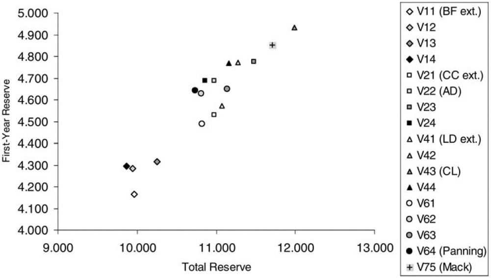
A subset of the pairs of reserves^[14] presented in Table 5 is plotted in Figure 1. Figure 1 shows that there is a strong positive correlation between the first-year reserves and the total reserves. Moreover, we make the following observations:

• Both reserves are low for the versions V11, V12, V13, V14 using the external prior estimators of the expected ultimate losses.

• Both reserves are relatively low for the versions V11, V21, V41, V61 using the external prior estimators of the quotas.

• Both reserves are relatively high for the versions V13, V23, V43, V63 using the chain-ladder quotas; this is due to the outlier in accident year 4 and development year 1.

• Both reserves are high for the versions V43 (chain-ladder method) and V75 (Mack’s method).^[15]

Moreover, there is a high volatility between the pairs of reserves produced by the different versions of the extended Bornhuetter-Ferguson method.

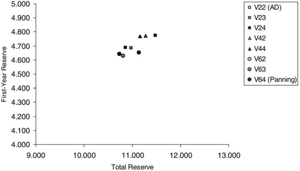
6.3. Reduction to reliable reserves

When combined with actuarial judgment, the previous observations may be used to select predictors providing reliable reserves:

• If the data of the run-off triangle are judged to be highly reliable, then the low predictors which are based of the external prior estimators of the expected ultimate losses and/or the quotas could be discarded.

• Since the predictors produced by the chain-ladder method and by Mack’s method are extremely high, they could be discarded as well.

• The remaining predictors provide ranges for the first-year reserve and for the total reserve which are not too large.

The remaining pairs of reserves could be judged as being reliable and are plotted in Figure 2. Figure 2 shows that the reliable pairs of reserves yield a rather small range for the first-year reserves (about 3% of the maximal value) and a slightly larger range for the total reserves (about 6% of the maximal value).

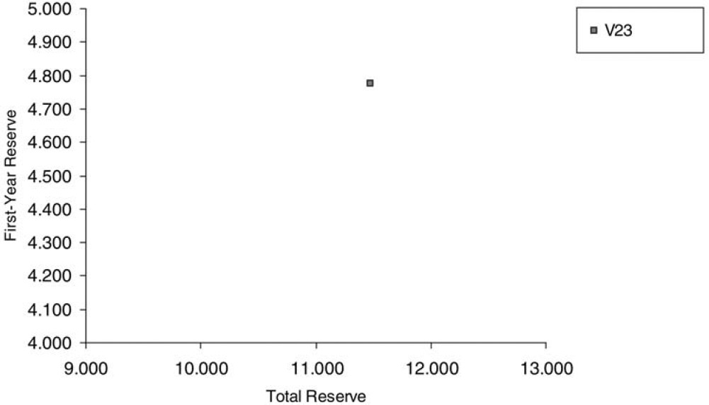
6.4. Selection of best reserves

Once the reliable reserves are determined, the final problem is to select predictors which can be regarded as best predictors of the ultimate losses. For example, if particularly prudent reserves are required, then one might select the predictors of version V23 (Cape Cod method with chain-ladder quotas) plotted in Figure 3. Of course, actuarial judgment could also lead to the selection of another version of the extended Bornhuetter-Ferguson method among those which produce reliable reserves.

6.5. Ranges

The selection of a particular version of the extended Bornhuetter-Ferguson method provides predictors which can be regarded as best predictors of the ultimate losses. However, the rules of accounting tend to require not only best predictors but also ranges reflecting the uncertainty of the best predictors.

The Bornhuetter-Ferguson principle also provides an approximate solution to this requirement: since the different versions of the extended Bornhuetter-Ferguson method generate a variety of reserves, they can be used to determine reliable ranges for the ultimate losses. These ranges are, of course, non-probabilistic ones; instead, they reflect the uncertainty caused by the different sources of information used in the different versions of the extended Bornhuetter-Ferguson method.

In our opinion, the ranges provided by the Bornhuetter-Ferguson principle could be more realistic than those obtained from additional and more or less artificial probabilistic assumptions like, e.g., the normal assumption for incremental losses.

6.6. Analysis of the run-off triangle

Beyond the selection of best predictors and ranges, the Bornhuetter-Ferguson principle may also be used to analyze the run-off triangle and hence the portfolio under consideration. We only mention two rather obvious aspects of such an analysis:

• In the case where the predictors based on (external) prior estimators obtained from a market portfolio differ significantly from the other predictors, the structure of the portfolio under consideration is likely to differ from the market portfolio.

• In the case where the predictors based on volume measures differ significantly from the other predictors, there might be something wrong with the volume measures; in particular, if the volume measures are premiums, then the difference between the predictors could indicate inappropriate pricing.

6.7. Refined analysis

The plot presented in Figure 1 is just one of various possibilities in analyzing the effects of the different versions of the extended Bornhuetter-Ferguson method. Other two-dimensional plots could be designed for representing certain pairs of predictors produced by the different versions of the extended Bornhuetter-Ferguson method and could be used for selecting best predictors and ranges or for analyzing the run-off triangle.

7. Proofs

The present section provides proofs of two non-obvious results mentioned in Subsections 5.6 and 5.7.

7.1. Additive method and Cape Cod method

The following result implies that the additive method with respect to the volume measure $\pi$ is identical to the Cape Cod method with respect to $\pi$ and the development pattern $\hat{\gamma}^{\mathrm{AD}}(\pi)$ :

Lemma The prior estimators of the additive method satisfy

$$\hat{\boldsymbol{\alpha}}^{\mathrm{AD}}(\pi)=\hat{\boldsymbol{\alpha}}^{\mathrm{CC}}\left(\pi, \hat{\gamma}^{\mathrm{AD}}(\pi)\right) .$$

Proof We have

$$\begin{array}{l} \left(\sum_{l=0}^{n} \hat{\zeta}_{l}^{\mathrm{AD}}(\pi)\right)\left(\sum_{j=0}^{n} \pi_{j} \hat{\gamma}_{n-j}^{\mathrm{AD}}(\pi)\right) \\ \quad=\sum_{j=0}^{n} \pi_{j} \sum_{l=0}^{n-j} \hat{\zeta}_{l}^{\mathrm{AD}}(\pi) \\ \quad=\sum_{l=0}^{n} \hat{\zeta}_{l}^{\mathrm{AD}}(\pi) \sum_{j=0}^{n-l} \pi_{j} \\ \quad=\sum_{l=0}^{n} \sum_{j=0}^{n-l} Z_{j, l} \\ \quad=\sum_{j=0}^{n} \sum_{l=0}^{n-j} Z_{j, l} \\ \quad=\sum_{j=0}^{n} S_{j, n-j} . \end{array}$$

This yields

$$\begin{aligned} \hat{\alpha}_{i}^{\mathrm{AD}}(\pi) & =\pi_{i} \sum_{l=0}^{n} \hat{\zeta}_{l}^{\mathrm{AD}}(\pi) \\ & =\pi_{i} \frac{\sum_{j=0}^{n} S_{j, n-j}}{\sum_{j=0}^{n} \pi_{j} \hat{\gamma}_{n-j}^{\mathrm{AD}}(\pi)} \\ & =\pi_{i} \hat{\kappa}^{\mathrm{CC}}\left(\pi, \hat{\gamma}^{\mathrm{AD}}(\pi)\right) \\ & =\hat{\alpha}_{i}^{\mathrm{CC}}\left(\pi, \hat{\gamma}^{\mathrm{AD}}(\pi)\right) \end{aligned}$$

as was to be shown.

7.2. Mack’s method and additive method

The following result implies that Mack’s method with respect to the volume measure $\pi$ is identical to the additive method with respect to the (adjusted) volume measure $\hat{\boldsymbol{\alpha}}^{\mathrm{LD}}\left(\gamma^{\mathrm{AD}}(\boldsymbol{\pi})\right):$

Lemma The prior estimators of Mack’s method satisfy

$$\hat{\gamma}^{\mathrm{Mack}}(\pi)=\hat{\gamma}^{\mathrm{AD}}\left(\hat{\boldsymbol{\alpha}}^{\mathrm{LD}}\left(\gamma^{\mathrm{AD}}(\pi)\right)\right.$$

and

$$\hat{\boldsymbol{\alpha}}^{\mathrm{Mack}}(\pi)=\hat{\boldsymbol{\alpha}}^{\mathrm{AD}}\left(\hat{\boldsymbol{\alpha}}^{\mathrm{LD}}\left(\gamma^{\mathrm{AD}}(\pi)\right)\right.$$

Proof We have

$$\begin{aligned} \pi_{i} \hat{Q}_{i}^{\mathrm{Mack}}(\pi) & =\pi_{i} \frac{\sum_{l=0}^{n-i} Z_{i, l}}{\sum_{l=0}^{n-i} \pi_{i} \hat{\zeta}_{l}^{\mathrm{AD}}(\pi)} \\ & =\frac{\sum_{l=0}^{n-i} Z_{i, l}}{\sum_{l=0}^{n-i} \hat{\zeta}_{l}^{\mathrm{AD}}(\pi)} \\ & =\frac{S_{i, n-i}}{\hat{\gamma}_{n-i}^{\mathrm{AD}}(\pi)} \frac{1}{\sum_{l=0}^{n} \hat{\zeta}_{l}^{\mathrm{AD}}(\pi)} \\ & =\hat{S}_{i, n}^{\mathrm{LD}}\left(\hat{\gamma}^{\mathrm{AD}}(\pi)\right) \frac{1}{\sum_{l=0}^{n} \hat{\zeta}_{l}^{\mathrm{AD}}(\pi)} \\ & =\hat{\alpha}_{i}^{\mathrm{LD}}\left(\hat{\gamma}^{\mathrm{AD}}(\pi)\right) \frac{1}{\sum_{l=0}^{n} \hat{\zeta}_{l}^{\mathrm{AD}}(\pi)} \end{aligned}$$

and hence

$$\begin{aligned} \hat{\zeta}_{k}^{\mathrm{Mack}}(\boldsymbol{\pi}) & =\frac{\sum_{j=0}^{n-k} Z_{j, k}}{\sum_{j=0}^{n-k} \pi_{j} \hat{\varrho}_{j}^{\mathrm{Mack}}(\boldsymbol{\pi})} \\ & =\frac{\sum_{j=0}^{n-k} Z_{j, k}}{\sum_{j=0}^{n-k} \hat{\alpha}_{j}^{\mathrm{LD}}\left(\hat{\gamma}^{\mathrm{AD}}(\boldsymbol{\pi})\right)} \sum_{l=0}^{n} \hat{\zeta}_{l}^{\mathrm{AD}}(\boldsymbol{\pi}) \\ & =\hat{\zeta}_{k}^{\mathrm{AD}}\left(\hat{\boldsymbol{\alpha}}^{\mathrm{LD}}\left(\hat{\gamma}^{\mathrm{AD}}(\boldsymbol{\pi})\right)\right) \sum_{l=0}^{n} \hat{\zeta}_{l}^{\mathrm{AD}}(\boldsymbol{\pi}) . \end{aligned}$$

This yields

$$\begin{aligned} \hat{\gamma}_{k}^{\mathrm{Mack}}(\pi) & =\frac{\sum_{l=0}^{k} \hat{\zeta}_{l}^{\mathrm{Mack}}(\pi)}{\sum_{l=0}^{n} \hat{\zeta}_{l}^{\mathrm{Mack}}(\pi)} \\ & =\frac{\sum_{l=0}^{k} \hat{\zeta}_{l}^{\mathrm{AD}}\left(\hat{\boldsymbol{\alpha}}^{\mathrm{LD}}\left(\hat{\gamma}^{\mathrm{AD}}(\pi)\right)\right)}{\sum_{l=0}^{n} \hat{\zeta}_{l}^{\mathrm{AD}}\left(\hat{\boldsymbol{\alpha}}^{\mathrm{LD}}\left(\hat{\gamma}^{\mathrm{AD}}(\pi)\right)\right)} \\ & =\hat{\gamma}_{k}^{\mathrm{AD}}\left(\hat{\boldsymbol{\alpha}}^{\mathrm{LD}}\left(\hat{\gamma}^{\mathrm{AD}}(\pi)\right)\right) \end{aligned}$$

and

$$\begin{aligned} \hat{\alpha}_{i}^{\mathrm{Mack}}(\boldsymbol{\pi}) & =\pi_{i} \hat{\kappa}_{i}^{\mathrm{Mack}}(\boldsymbol{\pi}) \\ & =\pi_{i} \hat{\varrho}_{i}(\boldsymbol{\pi}) \sum_{l=0}^{n} \hat{\zeta}_{l}^{\mathrm{Mack}}(\boldsymbol{\pi}) \\ & =\hat{\alpha}_{i}^{\mathrm{LD}}\left(\hat{\gamma}^{\mathrm{AD}}(\boldsymbol{\pi})\right) \sum_{l=0}^{n} \hat{\zeta}_{k}^{\mathrm{AD}}\left(\hat{\boldsymbol{\alpha}}^{\mathrm{LD}}\left(\hat{\gamma}^{\mathrm{AD}}(\boldsymbol{\pi})\right)\right) \\ & =\hat{\alpha}_{i}^{\mathrm{AD}}\left(\hat{\boldsymbol{\alpha}}^{\mathrm{LD}}\left(\hat{\gamma}^{\mathrm{AD}}(\boldsymbol{\pi})\right)\right) \end{aligned}$$

as was to be shown.

---

Acknowledgment

The authors gratefully acknowledge comments of Axel Reich and of three anonymous referees who helped substantially to clarify the intention of this paper.

---

1. Like the chain-ladder method and the Bornhuetter-Ferguson method, different methods of loss reserving address different target quantities. For the sake of comparison, it is necessary to express all methods in terms of the same target quantities. Our choice of focusing on ultimate losses (and later also on other cumulative losses) is essentially a matter of personal preferences.

2. The term prior in connection with the estimators of the cumulative quotas and the expected ultimate losses needs some explanation: It is used here only to indicate that these estimators are needed before the computation of the Bornhuetter-Ferguson predictors. Of course, the estimators of the expected ultimate losses could also be regarded as preliminary predictors of the ultimate losses, but this point is minor, and there will be no update of the estimators of the cumulative quotas.

3. This interpretation of the method proposed by Benktander (1976), which in fact is more general, follows Mack (2000). The Benktander method was rediscovered by Hovinen (1981) and a related paper is that of Neuhaus (1992).

4. The iterated Bornhuetter-Ferguson method is due to Mack (2000). With regard to terminology, it should be noted that in Mack (2000) the loss-development predictors presented in Subsection 5.3 are referred to as chain-ladder predictors.

5. The loss-development method provides a simple and useful extension of the chain-ladder method (see Subsection 5.4) and is sometimes referred to as the (generalized) chain-ladder method; see, e.g., Mack (2000). The loss-development method has been described in Radtke and Schmidt (2004) but it is likely that there are earlier sources in the literature.

6. An early source containing a description of the Cape Cod method is the monograph by Straub 1988) who refers in turn to an unpublished paper by Bühlmann (1983). The Cape Cod method was also mentioned by Stanard (1985) who refers to Stanard (1980) and Bühlmann (1983).

7. It is interesting to note that the Cape Cod predictors depend only on the relative size of the volume measures of the different accident years. In fact, for every c > 0, we have κ̂^CC(cπ, γ̂) = (1/c)κ̂^CC(π, γ̂), and hence Ŝ^CC(cπ, γ̂)= Ŝ^CC(π, γ̂).

8. The additive method was described by Mack (1997); see also Radtke and Schmidt (2004) where it is pointed out that the predictors of the additive method can be obtained as Gauss-Markov predictors in a suitable linear model.

9. It is interesting to note that, just like the Cape Cod predictors, the additive predictors depend only the relative size of the volume measures of the different accident years. In fact, for every c > 0, we have γ̂^AD(cπ)= γ̂^AD(π) and α̂^AD(cπ)= α̂^AD(π), and hence Ŝ^AD(cπ)= Ŝ^AD(π).

10. As it is the case for the additive method, it is easily seen that also the predictors of Mack’s method depend only on the relative size of the volume measures of the different accident years.

11. Since the adjusted volume measures are loss-development predictors of the ultimate losses, their order of magnitude usually differs from that of the initial volume measures. At first glance, this may cause some irritation, but it is resolved immediately because, as pointed out before, the prior estimators of the additive method depend only on the relative size of the volume measures.

12. Actually, Panning’s assumptions are stronger and are those of the homogeneous and homoscedastic conditional linear model for the incremental losses of every single development year with respect to the losses of the initial development year.

13. It is interesting to note that in Mack’s method different development patterns are used for the adjustment of the volume measure and the final application of the additive method with respect to the adjusted volume measure.

14. In order not to overcharge the plot, the pairs of reserves which are based on the prior estimators α̂^AD(π) or α̂^Panning*(γ̂) are omitted.

15. In the example, the reserves produced by the chain-ladder method and by Mack’s method are similar; this corresponds to the similarity of the development patterns γ̂^CL and γ̂^Mack given in Table 3 and to a remark of Mack (2006) indicating that a certain iteration of his method would approach the chain-ladder method.