1. Introduction
Copulas provide a convenient way to express multivariate distributions. Given the individual distribution functions Fi(Xi) the multivariate distribution can be expressed as a copula function applied to the probabilities, i.e., F(X1,…,Xn)=C[F1(X1),…,Fn(Xn)]. Venter (2002) discusses many of the basic issues of using copulas with the heavy-tailed distributions of property and liability (P&L) insurance. One of the key concepts is that copulas can control where in the range of probabilities the dependence is strongest. Any copula C is itself a multivariate distribution function but one that applies only to uniform distributions on the unit square, unit cube,…, depending on dimension. The uniform [0,1] variables are interpreted as probabilities from other distributions and are represented by U,V, etc.
One application is correlation in losses across lines of business. Lines tend to be weakly correlated in most cases but can be strongly correlated in extreme cases, like earthquakes. Belguise and Levi (2002) study copulas applied to catastrophe losses across lines. With financial modeling growing in importance, other potential applications of copulas in insurance company management include the modeling of dependence between loss and loss expense, dependence among asset classes, dependence among currency exchange rates, and credit risk among reinsurers.
The upper and lower tail dependence coefficients of a copula provide quantification of tail strength. These can be defined using the right and left tail concentration functions R and L on (0,1):
R(z)=Pr(U>z∣V>z)andL(z)=Pr(U<z∣V<z).
The upper tail dependence coefficient is the limit of R as z → 1, and the lower tail dependence coefficient is the limit of L as z → 0. For the normal copula and many others, these coefficients are zero. This means that for extreme values the distributions are uncorrelated, so large-large or small-small combinations are not likely. However, this is somewhat misleading, as the slopes of the R and L functions for the normal and t-copulas can be very steep near the limits. Thus there can be a significant degree of dependence near the limits even when it is zero at the limit. Thus looking at R(z) for z a bit less than 1 may be the best way to examine large loss dependencies.
While a variety of bivariate copulas is available, when more than two variables are involved the practical choice comes down to normal vs. t-copula. The normal copula is essentially the t-copula with high degrees of freedom (df), so the choice is basically what df to use in that copula. Venter (2003) discusses the use of the t-copula in insurance. The t takes a correlation parameter for each pair of variates, and any correlation matrix can be used. The df parameter adds a common-shock effect. This can be seen in the simulation methodology, where first a vector of multivariate normal deviates is simulated then the vector is multiplied by a draw from a single inverse gamma distribution. The df parameter is the shape parameter of the latter distribution, which is more heavy tailed with lower df. The factor drawn represents a common shock that hits all the normal variates with the same factor. This increases tail dependence in both the right and left tails but also increases the likelihood of anti-correlated results, so the overall correlation stays the same as in the normal copula.
Two problems for the t-copula are the symmetry between right and left tails and having only a single df parameter. The stronger tail dependence in insurance tends to happen in the right tail. Putting the same dependence in the left tail would be inaccurate, but it would probably have little effect on risk measurement overall, which is largely affected by the right tail. The single df parameter is more of a restriction. It results in giving more tail dependence to more strongly correlated pairs. This is reasonable but is not always consistent with data.
Thus more flexible multivariate copulas would be useful. One alternative provided by Daul et al (2003). is the grouped t-copula, which uses different df parameters for different subgroups of variables, such as corporate bonds grouped by country. We introduce a special case of that called the individuated t-copula, or IT, which has a df parameter for each variable. Another direction is that of Joe (1997), who develops a method for combining simple copulas to build up multivariate copulas. Three of these–called MM1, MM2, and MM3–have closed-form expressions. We investigate some of the properties of these copulas.
The t-copula for n variates has (n2 − n + 2)/2 parameters. The MMC copulas have one more parameter for each variate and so have (n2 + n + 2)/2 all together, while the IT has (n2 + n)/2. This situation does not include enough parameters to have separate control of the strength of the tail dependency for every pair of variates, but it does add some flexibility. The IT copula generalizes the t so it can be tried any time the t is too limiting in the possibilities for tail behavior. The MMC copulas have a parameter for each pair of variates, but this does not give them full flexibility in matching a covariance matrix. When all the bivariate correlations are fairly low (below 50% in the trivariate case but decreasing with more dimensions) they can usually all be matched, but the higher they get the more similar they are forced to be. This would probably be fine for insurance losses by line of business, as they tend to have low correlations overall but can be related when the losses are large. In modeling them, some additional flexibility in tail behavior vs. overall correlation could be helpful, so this could be an application where the MMC copulas would have an advantage over the t-copula.
2. IT copula
This copula is most readily described by the simulation procedure from its parameters, which are a correlation matrix ρ and a parameter νn for each of the N variables. The simulation starts with the generation of a multivariate normal vector {zn} with correlation matrix ρ by the usual approach (Cholesky decomposition, etc.). Then a uniform (0,1) variate u is drawn. The inverse chi-squared distribution quantile with probability u and df νn, denoted by wn=hn(u), is calculated. Then tn=zn[νn/wn]1/2 is t-distributed with νn df. To get the copula value, which is a probability, that t-distribution is applied to tn. The only difference between this and simulation of the t-copula is the t uses the same inverse chi-square draw for each variate.
The chi-squared distribution is a special case of the gamma. The ratio wn/νn is a scale transform of the chi-squared variate, so is a gamma variate. If the gamma density is parameterized to be proportional to xα−1e−x/β, then wn/νn has parameters β=2/νn and α=νn/2. This is a distribution with mean 1. It can be simulated easily if an inverse gamma function is available, as in some spreadsheets. It is not necessary for the df to be an integer for this to work. If not an integer, a beta distribution can be used to calculate the t-distribution probability, as in Venter (2003).
Although the simulation is straightforward, the copula density and probability functions are somewhat complicated. In terms of hn, the inverse chi-squared function above, and denoting the matrix inverse of ρ as J and the inverse t-distribution of un with νn df as tn, the copula density at (u1,…,un) can be shown to be:
c(→u)=∫10∏Nn=1{√hn(y)Γ(νn/2)(1+t2nνn)(1+νn)/2/Γ(1+νn2)}√det(ρ)(2π)Nexp(∑n,mJn,mtntm2√hn(y)hm(y)νnνm)dy.
This has to be computed numerically unless the df parameters are all the same, in which case it reduces to the t-copula density.
Daul et al (2003). find that the correlations (Spearman’s rho and Kendall’s tau) are not exactly the same as for the t-copula, but are quite close. Also the bivariate t-copula right and left dependence coefficients are Sn+1{[(n+1)(1−ρ)/(1+ρ)]0.5} where Sn+1 is the t-distribution survival function (PrX>x) with n+1df. If we denote the bivariate standard normal survival function as S(x,y)=Pr(X>x,Y>y), then the tail dependence coefficients for Xm and Xn for the IT copula are:
∫∞0S(cny1/νn,cmy1/νm)dy where cj=√2[Γ(1+νj2)/√4π]1/νj.
These tend to be between the t-copula dependence coefficients for the two dfs but closer to that for the higher of the two dfs if these are very different.
Fitting the IT by maximum likelihood is possible but involves several numerical steps. Alternatively, the df parameter for the t-copula could be estimated for each pair of variables by matching tail behavior, as in Venter (2003), and then individual dfs assigned to be consistent with this. Daul et al (2003). propose separate t-copulas for different groups of variables, which are combined into a single copula with the overall correlation matrix and the separate dfs.
3. MMC copulas
Joe’s MM1, MM2, and MM3 copulas each have an overall strength parameter θ, a parameter for each pair of variables δij (not the Kronecker delta), and add an additional parameter pj, with 1/pj≥m−1, for each of the m variables Uj, which gives the possibility of more control over the tails.
The parameters are then δij for i<j,pj, for j=1,…,m, and θ. For each variable uj, it is convenient to use the abbreviations yj=(−lnuj)θ and wj=pj(u−θj−1). The δij parameters would seem to allow for a correlation matrix, but it turns out that there are restrictions on how different the correlations can be, with the θ parameter exerting a lot of control. In effect, the parameters do not have as much freedom to fit to data as might be desired. The copula functions and dependency coefficients are given below. The density functions for the copulas needed for maximum likelihood estimation (MLE) are discussed in Appendix 1. Appendix 2 discusses numerical evaluation of MLE and rejection sampling (Tillé 1996) as a method for assessing standard errors.
MM1
Here δij≥1 and θ≥1. The copula at the m vector u is:
C(u)=exp{−[∑mj=1(1−(m−1)pj)yj+∑i<j((piyi)δij+(pjyj)δij)1/δij]1/θ}
The bivariate i, j margin is:
C(ui,uj)=exp{−[(1−pi)yi+(1−pj)yj+((piyi)δij+(pjyj)δij)1/δij]1/θ}
Lower tail dependence is zero. Upper tail dependence is given by:
λij=2−[2+(pδiji+pδijj)1/δij−pi−pj]1/θ
MM2
Here δij>0 and θ>0. The copula at the m vector u is:
C(u)=[m∑j=1u−θj+1−m−∑i<j(w−δiji+w−δijj)−1/δij]−1/θ
The i, j margin is:
C(ui,uj)=[u−θi+u−θj−1−(w−δiji+w−δijj)−1/δij]−1/θ
Because both upper and lower tail dependence are positive for this copula, a subscript is used to distinguish them here. The upper tail dependence is:
λij,U=(p−δiji+p−δijj)−1/δij
The lower tail dependence is:
λij,L=[2−(p−δiji+p−δijj)−1/δij]−1/θ
MM3
This starts with δij>0 and θ>1 (Although Joe says θ>0 is allowed, we have had problems if θ<1.). The copula at u is
C(u)=exp{−[m∑j=1yj−∑i<j((piyi)−δij+(pjyj)−δij)−1/δij]1/θ}
The i, j margin is
C(ui,uj)=exp{−[yi+yj−((piyi)−δij+(pjyj)−δij)−1/δij]1/θ}
The upper tail dependence is:
λij=2−[2−(p−δiji+p−δijj)−1/δij]1/θ
4. Range of possible correlations and dependencies
It turns out that not every possible correlation matrix can be matched by these copulas. The θ parameter determines a lot of what is possible for each copula. Tables 1–6 show the tail dependence and Spearman’s ρ for selected parameters.
For MM1 and MM3 the lower tail dependence is zero, so it is not shown. It is shown for MM2, but there the upper dependence does not depend on θ, so “any” is shown for θ.
Table 1.MM1 upper tail dependence
| pi |
pj:.005 |
.17 |
.335 |
.5 |
.005 |
.17 |
.335 |
.5 |
.005 |
.17 |
.335 |
.5 |
.005 |
.17 |
.335 |
.5 |
.005 |
.17 |
.335 |
.5 |
| 1.01 |
.005 |
.049 |
.049 |
.049 |
.049 |
.134 |
.134 |
.134 |
.134 |
.318 |
.318 |
.318 |
.318 |
.586 |
.586 |
.586 |
.586 |
.811 |
.811 |
.811 |
.811 |
| 1.01 |
.17 |
.049 |
.051 |
.052 |
.052 |
.134 |
.136 |
.137 |
.137 |
.318 |
.320 |
.320 |
.321 |
.586 |
.587 |
.587 |
.587 |
.811 |
.811 |
.811 |
.811 |
| 1.01 |
.335 |
.049 |
.052 |
.053 |
.054 |
.134 |
.137 |
.138 |
.139 |
.318 |
.320 |
.321 |
.322 |
.586 |
.587 |
.587 |
.588 |
.811 |
.811 |
.811 |
.812 |
| 1.01 |
.5 |
.049 |
.052 |
.054 |
.055 |
.134 |
.137 |
.139 |
.140 |
.318 |
.321 |
.322 |
.323 |
.586 |
.587 |
.588 |
.588 |
.811 |
.811 |
.812 |
.812 |
| 1.1 |
.005 |
.049 |
.051 |
.051 |
.051 |
.134 |
.135 |
.136 |
.136 |
.319 |
.319 |
.319 |
.320 |
.586 |
.586 |
.586 |
.587 |
.811 |
.811 |
.811 |
.811 |
| 1.1 |
.17 |
.051 |
.068 |
.076 |
.080 |
.135 |
.151 |
.158 |
.162 |
.319 |
.331 |
.336 |
.339 |
.586 |
.593 |
.596 |
.598 |
.811 |
.814 |
.815 |
.816 |
| 1.1 |
.335 |
.051 |
.076 |
.087 |
.095 |
.136 |
.158 |
.168 |
.176 |
.319 |
.336 |
.344 |
.349 |
.586 |
.596 |
.600 |
.603 |
.811 |
.815 |
.817 |
.818 |
| 1.1 |
.5 |
.051 |
.080 |
.095 |
.106 |
.136 |
.162 |
.176 |
.185 |
.320 |
.339 |
.349 |
.357 |
.587 |
.598 |
.603 |
.608 |
.811 |
.816 |
.818 |
.820 |
| 2 |
.005 |
.052 |
.054 |
.054 |
.054 |
.136 |
.138 |
.138 |
.138 |
.320 |
.321 |
.321 |
.321 |
.587 |
.588 |
.588 |
.588 |
.811 |
.812 |
.812 |
.812 |
| 2 |
.17 |
.054 |
.143 |
.171 |
.183 |
.138 |
.218 |
.243 |
.254 |
.321 |
.381 |
.400 |
.409 |
.588 |
.621 |
.632 |
.637 |
.812 |
.826 |
.831 |
.832 |
| 2 |
.335 |
.054 |
.171 |
.234 |
.269 |
.138 |
.243 |
.300 |
.331 |
.321 |
.400 |
.444 |
.468 |
.588 |
.632 |
.657 |
.671 |
.812 |
.831 |
.841 |
.847 |
| 2 |
.5 |
.054 |
.183 |
.269 |
.325 |
.138 |
.254 |
.331 |
.382 |
.321 |
.409 |
.468 |
.507 |
.588 |
.637 |
.671 |
.693 |
.812 |
.832 |
.847 |
.857 |
| 11 |
.005 |
.053 |
.054 |
.054 |
.054 |
.138 |
.138 |
.138 |
.138 |
.321 |
.321 |
.321 |
.321 |
.587 |
.588 |
.588 |
.588 |
.811 |
.812 |
.812 |
.812 |
| 11 |
.17 |
.054 |
.199 |
.209 |
.209 |
.138 |
.268 |
.277 |
.277 |
.321 |
.419 |
.427 |
.427 |
.588 |
.643 |
.647 |
.647 |
.812 |
.835 |
.837 |
.837 |
| 11 |
.335 |
.054 |
.209 |
.344 |
.365 |
.138 |
.277 |
.399 |
.417 |
.321 |
.427 |
.520 |
.534 |
.588 |
.647 |
.701 |
.709 |
.812 |
.837 |
.860 |
.864 |
| 11 |
.5 |
.054 |
.209 |
.365 |
.491 |
.138 |
.277 |
.417 |
.532 |
.321 |
.427 |
.534 |
.623 |
.588 |
.647 |
.709 |
.762 |
.812 |
.837 |
.864 |
.887 |
Table 2.MM1 Spearman’s ρ
| δ |
θ: |
1.037 |
1.037 |
1.037 |
1.037 |
1.111 |
1.111 |
1.111 |
1.111 |
1.333 |
1.333 |
1.333 |
1.333 |
2 |
2 |
2 |
2 |
4 |
4 |
4 |
4 |
| pi |
pj:.005 |
.17 |
.335 |
.5 |
.005 |
.17 |
.335 |
.5 |
.005 |
.17 |
.335 |
.5 |
.005 |
.17 |
.335 |
.5 |
.005 |
.17 |
.335 |
.5 |
| 1.01 |
.01 |
.053 |
.054 |
.054 |
.054 |
.149 |
.149 |
.149 |
.149 |
.364 |
.364 |
.364 |
.364 |
.682 |
.682 |
.682 |
.682 |
.913 |
.913 |
.913 |
.913 |
| 1.01 |
.17 |
.054 |
.056 |
.057 |
.057 |
.149 |
.151 |
.152 |
.152 |
.364 |
.365 |
.366 |
.366 |
.682 |
.683 |
.684 |
.684 |
.913 |
.913 |
.913 |
.913 |
| 1.01 |
.335 |
.054 |
.057 |
.058 |
.059 |
.149 |
.152 |
.153 |
.154 |
.364 |
.366 |
.367 |
.368 |
.682 |
.684 |
.684 |
.685 |
.913 |
.913 |
.913 |
.913 |
| 1.01 |
.5 |
.054 |
.057 |
.059 |
.061 |
.149 |
.152 |
.154 |
.155 |
.364 |
.366 |
.368 |
.369 |
.682 |
.684 |
.685 |
.685 |
.913 |
.913 |
.913 |
.913 |
| 1.1 |
.01 |
.054 |
.056 |
.056 |
.056 |
.149 |
.151 |
.151 |
.151 |
.364 |
.365 |
.365 |
.366 |
.682 |
.683 |
.683 |
.683 |
.913 |
.913 |
.913 |
.913 |
| 1.1 |
.17 |
.056 |
.075 |
.083 |
.088 |
.151 |
.168 |
.176 |
.181 |
.365 |
.379 |
.385 |
.389 |
.683 |
.691 |
.694 |
.696 |
.913 |
.915 |
.916 |
.917 |
| 1.1 |
.335 |
.056 |
.083 |
.096 |
.105 |
.151 |
.176 |
.187 |
.196 |
.365 |
.385 |
.394 |
.401 |
.683 |
.694 |
.699 |
.702 |
.913 |
.916 |
.917 |
.918 |
| 1.1 |
.5 |
.056 |
.088 |
.105 |
.117 |
.151 |
.181 |
.196 |
.207 |
.366 |
.389 |
.401 |
.409 |
.683 |
.696 |
.702 |
.707 |
.913 |
.917 |
.918 |
.920 |
| 2 |
.01 |
.056 |
.060 |
.060 |
.060 |
.151 |
.155 |
.155 |
.155 |
.366 |
.369 |
.369 |
.369 |
.683 |
.685 |
.685 |
.686 |
.913 |
.913 |
.914 |
.914 |
| 2 |
.17 |
.060 |
.148 |
.182 |
.203 |
.155 |
.235 |
.267 |
.286 |
.369 |
.430 |
.455 |
.470 |
.685 |
.717 |
.730 |
.739 |
.913 |
.923 |
.926 |
.929 |
| 2 |
.335 |
.060 |
.182 |
.245 |
.287 |
.155 |
.267 |
.324 |
.362 |
.369 |
.455 |
.498 |
.528 |
.685 |
.730 |
.753 |
.768 |
.914 |
.926 |
.933 |
.937 |
| 2 |
.5 |
.060 |
.203 |
.287 |
.348 |
.155 |
.286 |
.362 |
.417 |
.369 |
.470 |
.528 |
.570 |
.686 |
.739 |
.768 |
.790 |
.914 |
.929 |
.937 |
.943 |
| 11 |
.01 |
.057 |
.060 |
.061 |
.061 |
.152 |
.155 |
.155 |
.155 |
.366 |
.369 |
.369 |
.369 |
.684 |
.686 |
.686 |
.686 |
.913 |
.914 |
.914 |
.914 |
| 11 |
.17 |
.060 |
.179 |
.223 |
.246 |
.155 |
.263 |
.303 |
.325 |
.369 |
.451 |
.482 |
.500 |
.686 |
.727 |
.744 |
.754 |
.914 |
.925 |
.930 |
.933 |
| 11 |
.335 |
.061 |
.223 |
.312 |
.369 |
.155 |
.303 |
.383 |
.435 |
.369 |
.482 |
.542 |
.582 |
.686 |
.744 |
.774 |
.794 |
.914 |
.930 |
.938 |
.944 |
| 11 |
.5 |
.061 |
.246 |
.369 |
.457 |
.155 |
.325 |
.435 |
.514 |
.369 |
.500 |
.582 |
.641 |
.686 |
.754 |
.794 |
.823 |
.914 |
.933 |
.944 |
.952 |
Table 3.MM2 upper tail dependence and MM2 lower tail dependence
| δ |
|
MM2 Upper Tail Dependence |
MM2 Lower Tail Dependence |
| θ: |
any |
any |
any |
any |
.111 |
.111 |
.111 |
.111 |
.333 |
.333 |
.333 |
.333 |
1 |
1 |
1 |
1 |
3 |
3 |
3 |
3 |
| pi |
pj:.005 |
.17 |
.335 |
.5 |
.005 |
.17 |
.335 |
.5 |
.005 |
.17 |
.335 |
.5 |
.005 |
.17 |
.335 |
.5 |
.005 |
.17 |
.335 |
.5 |
| .25 |
.005 |
.000 |
.001 |
.002 |
.002 |
.002 |
.002 |
.002 |
.002 |
.125 |
.125 |
.125 |
.125 |
.500 |
.500 |
.500 |
.500 |
.794 |
.794 |
.794 |
.794 |
| .25 |
.17 |
.001 |
.011 |
.015 |
.018 |
.002 |
.002 |
.002 |
.002 |
.125 |
.127 |
.128 |
.128 |
.500 |
.503 |
.504 |
.504 |
.794 |
.795 |
.796 |
.796 |
| .25 |
.335 |
.002 |
.015 |
.021 |
.025 |
.002 |
.002 |
.002 |
.002 |
.125 |
.128 |
.129 |
.130 |
.500 |
.504 |
.505 |
.506 |
.794 |
.796 |
.796 |
.797 |
| .25 |
.5 |
.002 |
.018 |
.025 |
.031 |
.002 |
.002 |
.002 |
.002 |
.125 |
.128 |
.130 |
.131 |
.500 |
.504 |
.506 |
.508 |
.794 |
.796 |
.797 |
.798 |
| 1 |
.005 |
.003 |
.005 |
.005 |
.005 |
.002 |
.002 |
.002 |
.002 |
.125 |
.126 |
.126 |
.126 |
.501 |
.501 |
.501 |
.501 |
.794 |
.794 |
.794 |
.794 |
| 1 |
.17 |
.005 |
.085 |
.113 |
.127 |
.002 |
.003 |
.003 |
.004 |
.126 |
.142 |
.149 |
.152 |
.501 |
.522 |
.530 |
.534 |
.794 |
.805 |
.809 |
.811 |
| 1 |
.335 |
.005 |
.113 |
.168 |
.201 |
.002 |
.003 |
.004 |
.005 |
.126 |
.149 |
.163 |
.172 |
.501 |
.530 |
.546 |
.556 |
.794 |
.809 |
.817 |
.822 |
| 1 |
.5 |
.005 |
.127 |
.201 |
.250 |
.002 |
.004 |
.005 |
.006 |
.126 |
.152 |
.172 |
.187 |
.501 |
.534 |
.556 |
.571 |
.794 |
.811 |
.822 |
.830 |
| 4 |
.005 |
.004 |
.005 |
.005 |
.005 |
.002 |
.002 |
.002 |
.002 |
.126 |
.126 |
.126 |
.126 |
.501 |
.501 |
.501 |
.501 |
.794 |
.794 |
.794 |
.794 |
| 4 |
.17 |
.005 |
.143 |
.167 |
.169 |
.002 |
.004 |
.004 |
.004 |
.126 |
.156 |
.162 |
.163 |
.501 |
.538 |
.546 |
.546 |
.794 |
.814 |
.817 |
.817 |
| 4 |
.335 |
.005 |
.167 |
.282 |
.320 |
.002 |
.004 |
.008 |
.009 |
.126 |
.162 |
.197 |
.211 |
.501 |
.546 |
.582 |
.595 |
.794 |
.817 |
.835 |
.841 |
| 4 |
.5 |
.005 |
.169 |
.320 |
.420 |
.002 |
.004 |
.009 |
.016 |
.126 |
.163 |
.211 |
.254 |
.501 |
.546 |
.595 |
.633 |
.794 |
.817 |
.841 |
.859 |
| 16 |
.005 |
.005 |
.005 |
.005 |
.005 |
.002 |
.002 |
.002 |
.002 |
.126 |
.126 |
.126 |
.126 |
.501 |
.501 |
.501 |
.501 |
.794 |
.794 |
.794 |
.794 |
| 16 |
.17 |
.005 |
.163 |
.170 |
.170 |
.002 |
.004 |
.004 |
.004 |
.126 |
.161 |
.163 |
.163 |
.501 |
.544 |
.546 |
.546 |
.794 |
.816 |
.818 |
.818 |
| 16 |
.335 |
.005 |
.170 |
.321 |
.335 |
.002 |
.004 |
.009 |
.010 |
.126 |
.163 |
.211 |
.217 |
.501 |
.546 |
.596 |
.601 |
.794 |
.818 |
.841 |
.844 |
| 16 |
.5 |
.005 |
.170 |
.335 |
.479 |
.002 |
.004 |
.010 |
.023 |
.126 |
.163 |
.217 |
.284 |
.501 |
.546 |
.601 |
.657 |
.794 |
.818 |
.844 |
.870 |
Table 4.MM2 Spearman’s ρ
| pi |
pj:.005 |
.17 |
.335 |
.5 |
.005 |
.17 |
.335 |
.5 |
.005 |
.17 |
.335 |
.5 |
.005 |
.17 |
.335 |
.5 |
.005 |
.17 |
.335 |
.5 |
| .25 |
.005 |
.028 |
.029 |
.029 |
.029 |
.079 |
.080 |
.081 |
.081 |
.213 |
.214 |
.214 |
.214 |
.479 |
.479 |
.479 |
.480 |
.787 |
.787 |
.787 |
.787 |
| .25 |
.17 |
.029 |
.039 |
.043 |
.047 |
.080 |
.090 |
.094 |
.097 |
.214 |
.222 |
.226 |
.229 |
.479 |
.485 |
.488 |
.490 |
.787 |
.790 |
.791 |
.792 |
| .25 |
.335 |
.029 |
.043 |
.050 |
.055 |
.081 |
.094 |
.101 |
.106 |
.214 |
.226 |
.232 |
.236 |
.479 |
.488 |
.492 |
.495 |
.787 |
.791 |
.793 |
.794 |
| .25 |
.5 |
.029 |
.047 |
.055 |
.062 |
.081 |
.097 |
.106 |
.112 |
.214 |
.229 |
.236 |
.241 |
.480 |
.490 |
.495 |
.499 |
.787 |
.792 |
.794 |
.796 |
| 1 |
.005 |
.030 |
.034 |
.034 |
.034 |
.081 |
.085 |
.085 |
.085 |
.214 |
.218 |
.218 |
.218 |
.480 |
.482 |
.483 |
.483 |
.787 |
.788 |
.788 |
.789 |
| 1 |
.17 |
.034 |
.113 |
.144 |
.164 |
.085 |
.160 |
.190 |
.209 |
.218 |
.284 |
.310 |
.326 |
.482 |
.527 |
.546 |
.557 |
.788 |
.808 |
.815 |
.821 |
| 1 |
.335 |
.034 |
.144 |
.200 |
.238 |
.085 |
.190 |
.243 |
.280 |
.218 |
.310 |
.356 |
.387 |
.483 |
.546 |
.577 |
.599 |
.788 |
.815 |
.829 |
.838 |
| 1 |
.5 |
.034 |
.164 |
.238 |
.291 |
.085 |
.209 |
.280 |
.331 |
.218 |
.326 |
.387 |
.432 |
.483 |
.557 |
.599 |
.629 |
.789 |
.821 |
.838 |
.851 |
| 4 |
.005 |
.031 |
.034 |
.035 |
.035 |
.082 |
.086 |
.086 |
.086 |
.215 |
.218 |
.219 |
.219 |
.480 |
.483 |
.483 |
.483 |
.787 |
.789 |
.789 |
.789 |
| 4 |
.17 |
.034 |
.152 |
.195 |
.219 |
.086 |
.197 |
.239 |
.262 |
.218 |
.315 |
.352 |
.372 |
.483 |
.548 |
.574 |
.588 |
.789 |
.816 |
.827 |
.833 |
| 4 |
.335 |
.035 |
.195 |
.282 |
.338 |
.086 |
.239 |
.322 |
.375 |
.219 |
.352 |
.423 |
.469 |
.483 |
.574 |
.621 |
.652 |
.789 |
.827 |
.846 |
.859 |
| 4 |
.5 |
.035 |
.219 |
.338 |
.424 |
.086 |
.262 |
.375 |
.456 |
.219 |
.372 |
.469 |
.539 |
.483 |
.588 |
.652 |
.698 |
.789 |
.833 |
.859 |
.878 |
| 16 |
.005 |
.031 |
.034 |
.035 |
.035 |
.082 |
.086 |
.086 |
.086 |
.215 |
.219 |
.219 |
.219 |
.480 |
.483 |
.483 |
.483 |
.787 |
.789 |
.789 |
.789 |
| 16 |
.17 |
.034 |
.157 |
.202 |
.225 |
.086 |
.202 |
.245 |
.268 |
.219 |
.320 |
.357 |
.377 |
.483 |
.551 |
.577 |
.592 |
.789 |
.817 |
.828 |
.835 |
| 16 |
.335 |
.035 |
.202 |
.294 |
.352 |
.086 |
.245 |
.333 |
.388 |
.219 |
.357 |
.432 |
.480 |
.483 |
.577 |
.627 |
.659 |
.789 |
.828 |
.848 |
.862 |
| 16 |
.5 |
.035 |
.225 |
.352 |
.443 |
.086 |
.268 |
.388 |
.474 |
.219 |
.377 |
.480 |
.554 |
.483 |
.592 |
.659 |
.708 |
.789 |
.835 |
.862 |
.882 |
Table 5.MM3 upper tail dependence
| pi |
pj:.005 |
.17 |
.335 |
.5 |
.005 |
.17 |
.335 |
.5 |
.005 |
.17 |
.335 |
.5 |
.005 |
.17 |
.335 |
.5 |
.005 |
.17 |
.335 |
.5 |
| .25 |
.005 |
.049 |
.050 |
.050 |
.050 |
.134 |
.135 |
.135 |
.135 |
.318 |
.319 |
.319 |
.319 |
.586 |
.586 |
.586 |
.586 |
.811 |
.811 |
.811 |
.811 |
| .25 |
.17 |
.050 |
.059 |
.063 |
.065 |
.135 |
.143 |
.146 |
.149 |
.319 |
.325 |
.327 |
.329 |
.586 |
.590 |
.591 |
.592 |
.811 |
.812 |
.813 |
.813 |
| .25 |
.335 |
.050 |
.063 |
.069 |
.073 |
.135 |
.146 |
.152 |
.155 |
.319 |
.327 |
.331 |
.334 |
.586 |
.591 |
.593 |
.595 |
.811 |
.813 |
.814 |
.815 |
| .25 |
.5 |
.050 |
.065 |
.073 |
.078 |
.135 |
.149 |
.155 |
.160 |
.319 |
.329 |
.334 |
.338 |
.586 |
.592 |
.595 |
.597 |
.811 |
.813 |
.815 |
.815 |
| 1 |
.005 |
.051 |
.053 |
.054 |
.054 |
.136 |
.138 |
.138 |
.138 |
.320 |
.321 |
.321 |
.321 |
.587 |
.588 |
.588 |
.588 |
.811 |
.812 |
.812 |
.812 |
| 1 |
.17 |
.053 |
.129 |
.155 |
.168 |
.138 |
.205 |
.229 |
.241 |
.321 |
.372 |
.390 |
.399 |
.588 |
.616 |
.626 |
.631 |
.812 |
.824 |
.828 |
.830 |
| 1 |
.335 |
.054 |
.155 |
.207 |
.238 |
.138 |
.229 |
.275 |
.303 |
.321 |
.390 |
.425 |
.446 |
.588 |
.626 |
.646 |
.659 |
.812 |
.828 |
.837 |
.842 |
| 1 |
.5 |
.054 |
.168 |
.238 |
.285 |
.138 |
.241 |
.303 |
.345 |
.321 |
.399 |
.446 |
.478 |
.588 |
.631 |
.659 |
.677 |
.812 |
.830 |
.842 |
.850 |
| 4 |
.005 |
.053 |
.054 |
.054 |
.054 |
.137 |
.138 |
.138 |
.138 |
.321 |
.321 |
.321 |
.321 |
.587 |
.588 |
.588 |
.588 |
.811 |
.812 |
.812 |
.812 |
| 4 |
.17 |
.054 |
.184 |
.207 |
.209 |
.138 |
.254 |
.275 |
.277 |
.321 |
.409 |
.425 |
.426 |
.588 |
.637 |
.646 |
.647 |
.812 |
.833 |
.836 |
.837 |
| 4 |
.335 |
.054 |
.207 |
.315 |
.351 |
.138 |
.275 |
.372 |
.405 |
.321 |
.425 |
.499 |
.524 |
.588 |
.646 |
.689 |
.704 |
.812 |
.836 |
.855 |
.862 |
| 4 |
.5 |
.054 |
.209 |
.351 |
.446 |
.138 |
.277 |
.405 |
.491 |
.321 |
.426 |
.524 |
.591 |
.588 |
.647 |
.704 |
.743 |
.812 |
.837 |
.862 |
.879 |
| 16 |
.005 |
.053 |
.054 |
.054 |
.054 |
.138 |
.138 |
.138 |
.138 |
.321 |
.321 |
.321 |
.321 |
.587 |
.588 |
.588 |
.588 |
.812 |
.812 |
.812 |
.812 |
| 16 |
.17 |
.054 |
.202 |
.209 |
.209 |
.138 |
.271 |
.277 |
.277 |
.321 |
.422 |
.427 |
.427 |
.588 |
.645 |
.647 |
.647 |
.812 |
.836 |
.837 |
.837 |
| 16 |
.335 |
.054 |
.209 |
.352 |
.365 |
.138 |
.277 |
.406 |
.418 |
.321 |
.427 |
.525 |
.534 |
.588 |
.647 |
.704 |
.710 |
.812 |
.837 |
.862 |
.864 |
| 16 |
.5 |
.054 |
.209 |
.365 |
.501 |
.138 |
.277 |
.418 |
.541 |
.321 |
.427 |
.534 |
.630 |
.588 |
.647 |
.710 |
.767 |
.812 |
.837 |
.864 |
.889 |
Table 6.MM3 Spearman’s ρ
| pi |
pj:.005 |
.17 |
.335 |
.5 |
.005 |
.17 |
.335 |
.5 |
.005 |
.17 |
.335 |
.5 |
.005 |
.17 |
.335 |
.5 |
.005 |
.17 |
.335 |
.5 |
| .25 |
.005 |
.054 |
.055 |
.055 |
.055 |
.148 |
.150 |
.150 |
.150 |
.363 |
.365 |
.365 |
.365 |
.682 |
.683 |
.683 |
.683 |
.912 |
.913 |
.913 |
.913 |
| .25 |
.17 |
.055 |
.065 |
.069 |
.072 |
.150 |
.159 |
.163 |
.166 |
.365 |
.372 |
.375 |
.377 |
.683 |
.687 |
.689 |
.690 |
.913 |
.914 |
.914 |
.915 |
| .25 |
.335 |
.055 |
.069 |
.076 |
.081 |
.150 |
.163 |
.169 |
.174 |
.365 |
.375 |
.380 |
.384 |
.683 |
.689 |
.691 |
.693 |
.913 |
.914 |
.915 |
.916 |
| .25 |
.5 |
.055 |
.072 |
.081 |
.087 |
.150 |
.166 |
.174 |
.180 |
.365 |
.377 |
.384 |
.388 |
.683 |
.690 |
.693 |
.696 |
.913 |
.915 |
.916 |
.917 |
| 1 |
.005 |
.051 |
.060 |
.060 |
.060 |
.146 |
.154 |
.155 |
.155 |
.362 |
.368 |
.369 |
.369 |
.681 |
.685 |
.685 |
.685 |
.912 |
.913 |
.914 |
.914 |
| 1 |
.17 |
.060 |
.137 |
.168 |
.187 |
.154 |
.225 |
.253 |
.271 |
.368 |
.423 |
.445 |
.459 |
.685 |
.713 |
.725 |
.733 |
.913 |
.922 |
.925 |
.927 |
| 1 |
.335 |
.060 |
.168 |
.222 |
.259 |
.155 |
.253 |
.303 |
.336 |
.369 |
.445 |
.483 |
.509 |
.685 |
.725 |
.745 |
.759 |
.914 |
.925 |
.931 |
.934 |
| 1 |
.5 |
.060 |
.187 |
.259 |
.311 |
.155 |
.271 |
.336 |
.384 |
.369 |
.459 |
.509 |
.545 |
.685 |
.733 |
.759 |
.778 |
.914 |
.927 |
.934 |
.940 |
| 4 |
.005 |
.050 |
.060 |
.061 |
.061 |
.146 |
.155 |
.155 |
.155 |
.366 |
.369 |
.369 |
.369 |
.683 |
.686 |
.686 |
.686 |
.913 |
.914 |
.914 |
.914 |
| 4 |
.17 |
.060 |
.175 |
.217 |
.241 |
.155 |
.259 |
.298 |
.320 |
.369 |
.448 |
.479 |
.496 |
.686 |
.726 |
.742 |
.752 |
.914 |
.925 |
.929 |
.932 |
| 4 |
.335 |
.061 |
.217 |
.302 |
.357 |
.155 |
.298 |
.374 |
.424 |
.369 |
.479 |
.536 |
.574 |
.686 |
.742 |
.771 |
.790 |
.914 |
.929 |
.937 |
.943 |
| 4 |
.5 |
.061 |
.241 |
.357 |
.440 |
.155 |
.320 |
.424 |
.499 |
.369 |
.496 |
.574 |
.630 |
.686 |
.752 |
.790 |
.818 |
.914 |
.932 |
.943 |
.951 |
| 16 |
.005 |
.050 |
.060 |
.061 |
.061 |
.145 |
.155 |
.155 |
.155 |
.366 |
.369 |
.369 |
.369 |
.684 |
.686 |
.686 |
.686 |
.913 |
.914 |
.914 |
.914 |
| 16 |
.17 |
.060 |
.180 |
.224 |
.247 |
.155 |
.264 |
.304 |
.326 |
.369 |
.451 |
.483 |
.501 |
.686 |
.727 |
.744 |
.754 |
.914 |
.925 |
.930 |
.933 |
| 16 |
.335 |
.061 |
.224 |
.313 |
.370 |
.155 |
.304 |
.384 |
.436 |
.369 |
.483 |
.543 |
.583 |
.686 |
.744 |
.774 |
.794 |
.914 |
.930 |
.938 |
.944 |
| 16 |
.5 |
.061 |
.247 |
.370 |
.459 |
.155 |
.326 |
.436 |
.516 |
.369 |
.501 |
.583 |
.642 |
.686 |
.754 |
.794 |
.824 |
.914 |
.933 |
.944 |
.952 |
5. Discussion
The tables in the previous section are bivariate relationships. However, since the p parameters can be no greater than 1/(m − 1), the possible values of p, and so the range of possible correlations and tail dependencies, reduce as the dimension increases. The θ parameter in general has a great deal of influence over what any of these copulas can do. As θ gets higher, the other parameters have very little influence. Thus when it is high, all pairs of variables will have similar correlations and tail dependencies. This is the case for any of the correlation coefficients (linear, rank, tau) so we use the term “correlation” generically. When θ is low, however, it is not possible to have very high correlations. Thus, in general, these copulas can only apply when all pairs of variables have similar tails and correlations.
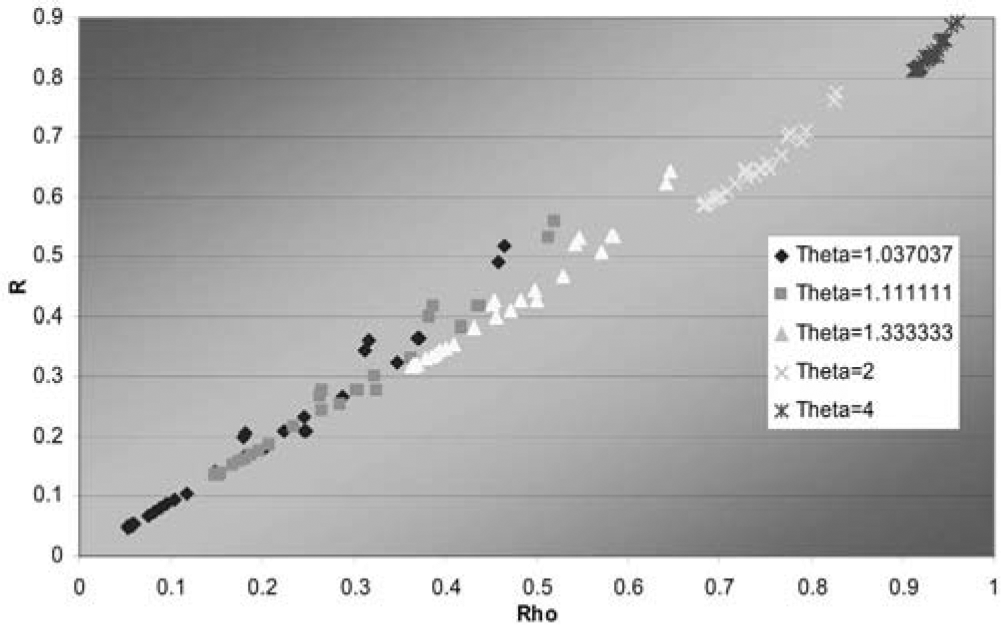
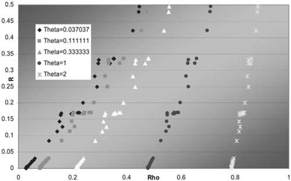
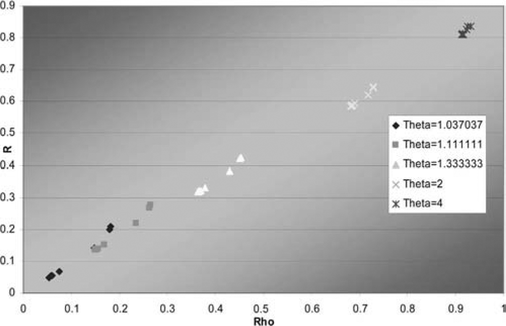
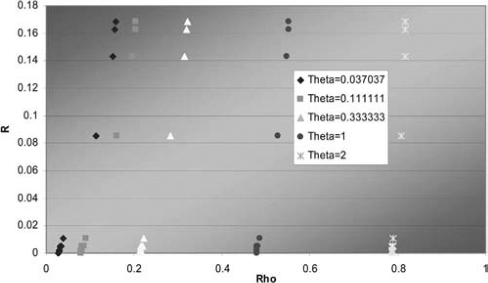
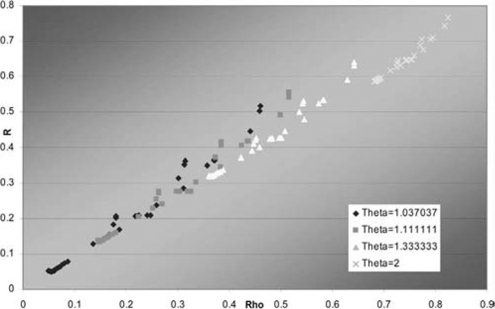
Also the right tail dependence R and the correlation are closely related. Scatterplots of R as a function of ρ for different values of θ are shown for the cases m = 3 and m = 7 for the MM1 and MM2 copulas and m = 7 for MM3 in Figures 1–5. These points are taken from the above tables so just give a suggestion of the spread in R available for the same values of ρ and θ. Even so, it is clear that some degree of variability of R is possible for pairs within a single copula even for the same rank correlation. This is in contrast to the t-copula for which the correlation and df determine the tail dependence uniquely.

Figure 1.MM1 R as a function of rho by theta, m=3

Figure 2.MM2 R as a function of rho by theta, m=3

Figure 3.MM1 R as a function of rho by theta, m=7

Figure 4.MM2 R as a function of rho by theta, m=7

Figure 5.MM2 R as a function of rho by theta, m=3
For MM2, R is not a function of θ, so a wider range of Rs is possible for any θ. The possible range of ρ for each θ is about the same for each copula. This range decreases with higher ms, however, due to the restricted range of p.
The relationship for MM3 in Figure 5 is similar to that for MM1 in Figure 1, but MM3 might have a bit more possible spread in R.
6. Fitting MM1 and MM2
As an example, we tried fitting the MM1 and MM2 copulas to currency rate changes. Currency data was chosen because it is publicly available, not because it is fit better by the MMC copulas. But by fitting to actual data, some of the shape differences among the copulas can be illustrated, as can fitting methods. The data consists of monthly changes in the US $ exchange rate for the Swedish, Japanese, and Canadian currencies from 1971 through September 2005. The data come from the Fred database of the St. Louis Federal Reserve. The Fred exchange rates were converted to monthly change factors, with a factor greater than 1.0 representing an appreciation of the US $ compared to that currency. These factors are comparative movements against the dollar, so if an event strengthens or weakens the dollar in particular, all the currencies would be expected to move in the same direction. Thus there could be common shocks.
The MMC copula densities get increasingly difficult to calculate as the dimension increases. For this reason, some alternatives to MLE were explored. One alternative is to maximize the product of the bivariate likelihood functions, which just requires the bivariate densities. Since the copulas are defined by the copula functions, an even easier fit is to minimize the distance between the empirical and fitted copulas, measured by sum of squared errors (SSE). Numerical differentiation, as discussed in Appendix 2, is another way to calculate the multivariate MLE but was not tried here.
The parameters for the various fitting methods are shown in Table 7. The product of the bivariate likelihood estimates for MM1 are quite close to the full trivariate MLE. It should be noted, however, that there are many local maxima for both likelihood functions, so we cannot be absolutely sure that these are the global maxima. Only the bivariate estimates were done for MM2. The SSE parameters are quite a bit different from the MLEs. Thus, the product of the bivariate MLEs appears to be the more promising shortcut method.
Table 7.Parameters for the various fitting methods
| SSE |
MLE bi |
SSE |
MLE bi |
MLE tri |
MLE bi |
MLE tri |
| δ12 |
2.62588 |
1.50608 |
3.69513 |
2.14275 |
2.1094 |
0.491 |
0.490 |
| δ13 |
0.80055 |
0.43963 |
1.52005 |
1.19832 |
1.1152 |
0.262 |
0.266 |
| δ23 |
3.2E-07 |
0.0103 |
1 |
1 |
1 |
0.097 |
0.097 |
| p1 |
0.49881 |
0.37649 |
0.49963 |
0.40533 |
0.37175 |
|
|
| p2 |
0.5 |
0.5 |
0.5 |
0.5 |
0.5 |
|
|
| p3 |
0.26236 |
0.49625 |
0.29097 |
0.5 |
0.5 |
|
|
| θ |
0.19599 |
0.2209 |
1.08308 |
1.0939 |
1.1234 |
20.53 |
20.95 |
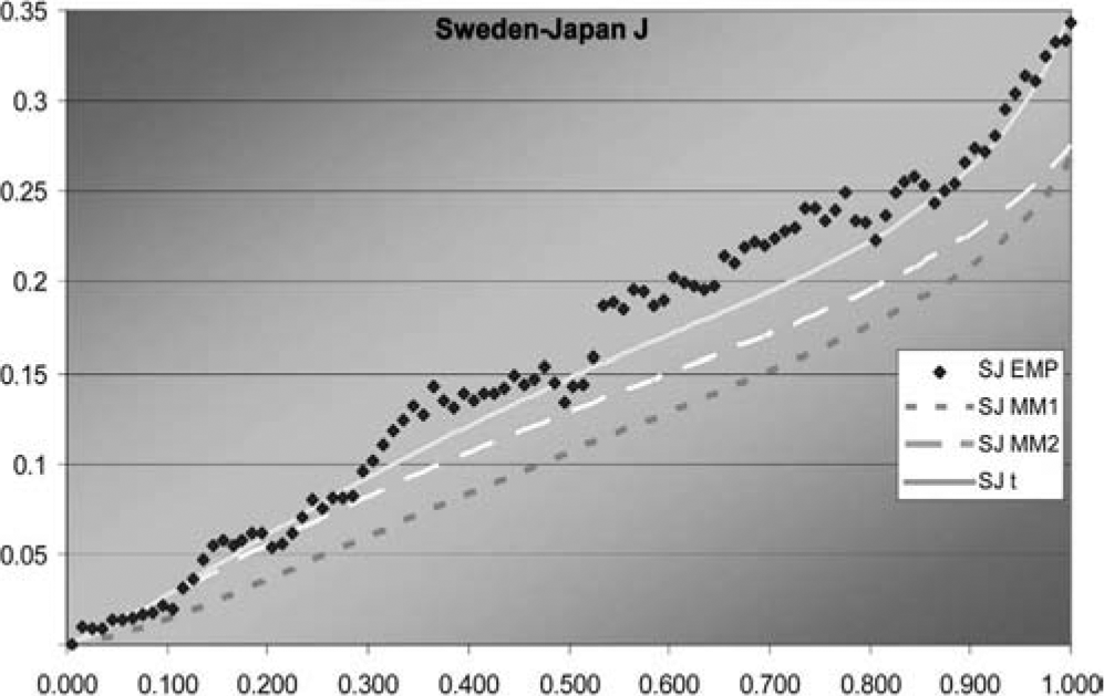
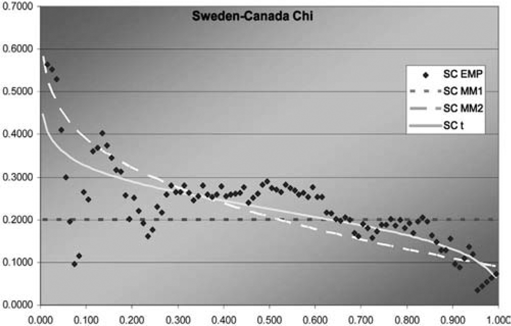
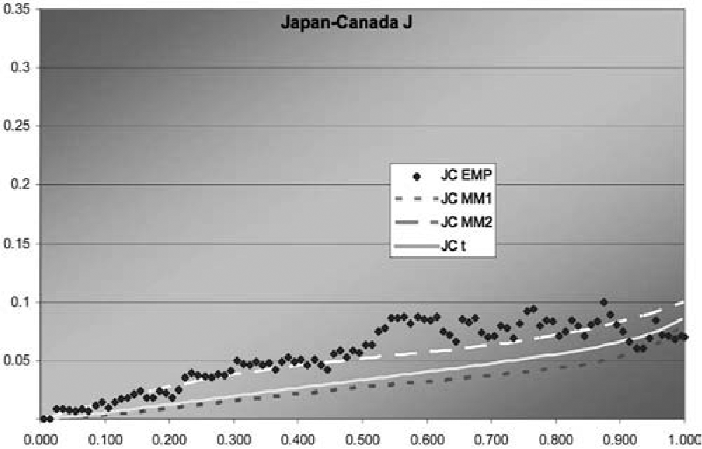
The t parameters were estimated by maximizing the trivariate and product of bivariate likelihood functions for comparison. We use a beta distribution version of the t that allows fractional degrees of freedom. Comparisons of fits were done using graphs of the empirical and fitted J and χ functions in Figures 6–11. These functions are defined as:
J(z)=−z2+4∫z0∫z0C(u,v)c(u,v)dvdu/C(z,z) and χ(z)=2−ln[C(z,z)]/lnz.
As z → 1 these approach Kendall’s r and the upper tail dependence R, respectively. They also can be compared to see the fit in the left tail, which is important for currency movements.

Figure 6.Sweden-Japan J function

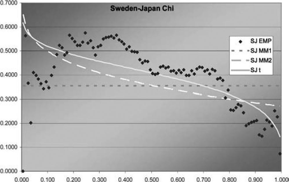
Figure 7.Sweden-Japan χ function

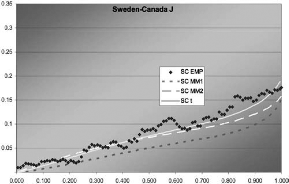
Figure 8.Sweden-Canada J function

Figure 9.Sweden-Canada χ function

Figure 10.Japan-Canada J function
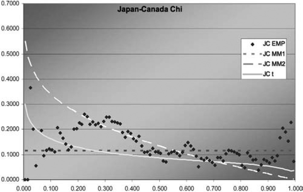
Figure 11.Japan-Canada χ function
In two of the three J graphs, the t-copula is clearly the best fit, but MM2 is close for Sweden-Canada. In the third, MM2 is the best. MM1 is always worse for this data. The t is also best in two of the three χ graphs, but not much better than MM2 for Sweden-Canada. In the third graph, each of the three is best in some range, but MM1 is probably best. Overall, MM2 seems to provide almost as good a fit as t, but not quite.
Although this dataset is fit best by the t-copula, that does not negate the value of having more than one multivariate copula available. The example explores methods of fitting multivariate copulas and comparing their fits, and illustrates the different shapes of the descriptive functions that can be produced by the different copulas. For exchange rates in particular, it may be worth exploring fitting the logs of the change factors by multivariate normal and t-distributions, as reciprocals of the factors are of interest and could have the same distribution.
7. Summary
The IT copula has potential for better fits when the t-copula tails differ. Trying to fit this to some actual data seems worthwhile.
The closed-form MMC copulas do not give full flexibility in the range of the bivariate correlations that can occur in a single multivariate copula. These copulas would be most appropriate when the empirical correlations are all fairly small or fairly close to each other. This gets more so as the number of dimensions increases. These copulas all have somewhat different shapes, and differ from the t-copula as well, so they could be useful with the right data. An interesting application may be to insurance losses by line of business, as their correlations are all relatively low and the tail dependences may not have the t-copula property of strictly growing with correlation. The correlations of losses across lines may not have the t’s symmetric right and left tails either, but this is less of a concern, as putting too much correlation into small losses is not likely to critically affect the properties of the distribution of the sum of the lines.
Joe also defines MM4 and MM5 copulas. These do not have closed-form expressions, but he asserts that they have a wide range of possible dependence. To build a larger repertoire of multivariate copulas, it may be worth developing algorithms for calculation and fitting these and trying them on live data.
Acknowledgments
We would like to acknowledge the contributions of Ka Chun Ma of Columbia University and David Strasser of Guy Carpenter in supporting the calculations in the paper and the quite useful suggestions of the anonymous reviewers from Variance, with the usual caveat.
Appendix
Appendix 1. MMC density functions
For maximum likelihood estimation, it would be desirable to have expressions for the copula densities, which are mixed partial derivatives of the copula C functions. Although it is difficult to write down general formulas for the densities, some broad outlines can be developed. Recall the product formula for derivatives (ab)′=a′b+b′a. Then (abc)′=(ab)′c+abc′=a′bc+ab′c+abc′. Similarly (abcd)′=a′bcd+ab′cd+abc′d+abcd′, etc. For any function F of the vector u, consider the simple multivariate function B(u)=F(u)a. Denoting partial derivatives with respect to the elements of u by subscripts, we have successively:
B=Fa.Bi=aFa−1Fi.Bij=a(a−1)Fa−2FiFj+aFa−1Fij.Bijk=a(a−1)(a−2)Fa−3FiFjFk+a(a−1)Fa−2×(FiFjk+FjFik+FkFij)+aFa−1Fijk.Bijkl=a(a−1)(a−2)(a−3)Fa−4FiFjFkFl+a(a−1)(a−2)Fa−3(FijFkFl+FikFjFl+FilFjFk+FjkFiFl+FjlFiFk+FklFiFj)+a(a−1)Fa−2(FiFjkl+FjFikl+FkFijl+FlFijk+FijFkl+FikFjl+FilFjk)+aFa−1Fijkl.
This is the form of the MM2 C function. Although a pattern is emerging in the subscripts, it seems difficult to write down a general rule for an arbitrary mixed partial.
A similar exercise can be carried out for C(u)=e−B(u).
C=e−B.C1=−CB1.C12=C(B1B2−B12).C123=C(B1B23+B2B13+B3B12−B1B2B3−B123).
C1234=C(B1B234+B2B134+B3B124+B4B123+B12B34+B13B24+B14B23−B12B3B4−B13B2B4−B14B2B3−B23B1B4−B24B1B3−B34B1B2+B1B2B3B4−B1234).
This is the form of the MM1 and MM3 C with Fa replacing B.
To calculate the derivatives let xj=y′j=θ(−lnuj)θ−1/uj, and tj=w′j=θpju−θ−1j. The case m=3 is not too bad. First for MM1:
F(u)=3∑j=1(1−2pj)yj+∑i<j((piyi)δij+(pjyj)δij)1/δij
Taking the first derivative:
Fi(u)=(1−2pj)yjxi+(piyi)δij−1pixi×∑j≠i((piyi)δij+(pjyj)δij)1/δij−1
This would be almost the same for the bivariate margin. Then:
Fij(u)=(1−δij)(pipjyiyj)δ−1ijpipjxixj×((piyi)δij+(pjyj)δij)1/δij−2
This is the same for the bivariate margin. From this it is clear that F123=0. Then taking a=1/θ and plugging in these values of Fi and Fij will give all values of Bi,Bij, and B123, which can then be plugged in the formula for C123 to give the density. From the formulas for C12 the bivariate density is similar.
MM2 is even easier, as the C formulas are not needed. What is needed is:
F(u)=3∑j=1u−θj−2−∑i<j(w−δiji+w−δijj)−1/δij
This gives:
Fi(u)=−θu−θ−1i−w−δij−1iti∑j≠i(w−δiji+w−δijj)−1/δij−1
And:
Fij(u)=−(1+δij)(wiwj)−δij−1titj(w−δiji+w−δijj)−1/δij−2
Again F123=0. Then setting a=−1/θ gives B123, which is the density.
This gets harder and harder as the dimension of u increases. Then numerical differentiation becomes increasingly attractive.
Appendix 2. Numerical densities
Background and notation
The discussion is oriented to copulas, i.e., smooth, parametric, cumulative distribution functions on the unit hypercube.
Let X∈Ω=[0,1]d with cdf F(X∣θ). Sample points are denoted x alone or x(i) if a sequence needs to be indexed. Components of x are xj.
From CDF to measure
Define the hypercube H(x,δ) as
([x1−δ/2,x1+δ/2]×[x2−δ/2,x2+δ/2]×⋯×[xd−δ/2,xd+δ/2])∩Ω
Without loss of generality, we may assume a generic H is wholly contained in Ω. We can identify the set of vertices of H(x,δ) with the set S={−1,1}d by the mapping
s=⟨s1,s2,…,sd⟩↦⟨x1+s1⋅δ/2,x2+s2⋅δ/2,…,xd+sd⋅δ/2⟩=C(x,δ,s).
Let g(s)=∏jsj be the sign of s.
Define the probability measure μ(H∣θ) as Pr{X∈H∣θ}.
Theorem
μ(H(x,δ)∣θ)=∑s∈Sg(s)⋅F(C(x,δ,s)∣Θ).
The probability of X being in a hypercube is the sum of the distribution function at positive corners minus its value at the negative corners. For d = 1 this is just the difference between the function at the top and bottom of the interval. For d = 2, this is the sum of the function at the upper right and lower left corners minus the function at each of the other corners. The latter two functions cover an overlapping area that gets subtracted twice, which is why you have to add back the function at the lower left. In general the proof requires keeping track of what are the positive and negative corners.
Proof For 0≤N≤d, define the hypersolids
HN=([x1−δ/2,x1+δ/2]×⋯×[xN−δ/2,xN+δ/2]×[0,xN+1+δ/2]×[0,xN+2+δ/2]×⋯×[0,xd+δ/2])H−N=([x1−δ/2,x1+δ/2]×⋯×[xN−δ/2,xN+δ/2]×[0,xN+1−δ/2]×[0,xN+2+δ/2]×⋯×[0,xd+δ/2])
and associated vertex index sets
SN={⟨±1,…,±1,1,1,…,1⟩} and S−N={⟨±1,…,±1,−1,1,…,1⟩},
respectively, each with 2N elements. There is a natural 1-to-1 mapping
s=⟨s1,…,sN,1,…,1⟩↦⟨s1,…,sN,−1,…,1⟩=s−
between SN and S−N.
We have that
μ(H0∣θ)=F(x1+δ/2,x2+δ/2,…,xd+δ/2)=∑s∈S0g(s)⋅F(C(x,δ,s)∣θ)
μ(H−0∣θ)=F(x1−δ/2,x2+δ/2,…,xd+δ/2)=−∑s∈S−0g(s)⋅F(C(x,δ,s)∣θ)
μ(H1∣θ)=μ(H0∖H−0∣θ)=μ(H0∣θ)−μ(H−0∣θ)=∑s∈S0g(s)⋅F(C(x,δ,s)∣θ)+∑s∈S−0g(s)⋅F(C(x,δ,s)∣θ)=∑s∈S1g(s)⋅F(C(x,δ,s)∣θ)
Assume that
μ(HN∣θ)=∑s∈SNg(s)⋅F(C(x,δ,s)∣θ).
The mapping s↦s−induces a correspondence between vertices of HN and H−N, and the fact that
μ(H−N∣θ)=−∑s∈S−Ng(s)⋅F(C(x,δ,s)∣θ)
follows by noting the change in sign between each g(s) and corresponding g(s−). Then
μ(HN+1∣θ)=μ(HN∖H−N∣θ)=μ(HN∣θ)−μ(H−N∣θ)=∑s∈SNg(s)⋅F(C(x,δ,s)∣θ)+∑s∈S−Ng(s)⋅F(C(x,δ,s)∣θ)=∑s∈SN+1g(s)⋅F(C(x,δ,s)∣θ)
By mathematical induction, it must be the case that
μ(Hd∣θ)=∑s∈Sdg(s)⋅F(C(x,δ,s)∣θ).
But Sd=S and the theorem is proved.
Approximating MLE
Since F is smooth, it has a probability density function defined by
f(x∣θ)≜
In general, this is intractable; i.e., a closed-form expression is not convenient. However, since \mu can be evaluated, a numerical approximation f(x \mid \theta, \delta) for small \delta is readily available by applying the theorem. Therefore, the log-likelihood of a set of data \left\{x^{(1)}, x^{(2)}, \ldots, x^{(n)}\right\} can be approximated by
\mathbf{L}(\theta) \approx \sum_{i} \ln \left(f\left(x^{(i)} \mid \theta, \delta\right)\right)
for suitably chosen δ.
This allows the application of standard MLE techniques.
Sampling
While MLE carries its own asymptotic results for assessing standard errors, it might be useful to conduct simulation experiments to bolster these results. A form of rejection sampling is outlined here. Say the goal is to sample n points from the distribution defined by F(· | θ).
Step 1 Choose N \gg n points x^{(i)} uniformly from \Omega.
Step 2 For each i, calculate \phi_i=f\left(x^{(i)} \mid \theta, \delta\right). Let m=\max \left\{\phi_i\right\} and M=\left(\Sigma \phi_i\right) / m. If M<n then go back to step 1 and choose a larger N.
Step 3 Sample n points without replacement from the discrete distribution \left\{\left\langle x^{(i)}, p_i\right\rangle\right\} where p_i=n * \phi_i /\left(\Sigma \phi_i\right). If you make sure the x^{(i)} are in random order, e.g., the order in which they were first sampled, you can use the following systematic sampling procedure:
Sample :=\{ \} . \mathrm{Sp}:=0 . \mathrm{i}:=0.
Repeat
i:=i+1 .
If the interval ( \mathrm{Sp}, \mathrm{Sp}+\mathrm{pi} ] contains an integer, then Sample := Sample \cup\left\{x^{(i)}\right\}.
S p:=S p+p_i
Until S p=n.