Modeling Mortgage Insurance as a Multistate Process

undefined

1. Introduction

This paper is concerned with modeling mortgage insurance claims experience. Most of its content applies to mortgage insurance generally, though in some places comment will be slanted toward insurance of residential, as opposed to commercial, mortgages.

Mortgage insurance indemnifies the lender against loss in the event of default under a mortgage leading to sale of the collateral property. A loss would occur if the proceeds of the sale, less its costs, were insufficient to defray the amount outstanding in respect of the mortgage loan. In the parlance of the financial markets, a mortgage insurance contract is a credit default swap (Saunders and Allen 2002).

This line of business has a number of relatively unique properties:

• Policies provide multiyear coverage in return for a single premium.

• The claims experience is strongly influenced by variables that relate specifically to the housing sector of the economy.

• A claim occurs at the end of a defined sequence of events, somewhat different from those of other lines.

Subsequent sections address this single-premium form of contract. In cases where premiums are paid periodically, some details of the paper, particularly in Section 6.1 on earning of premium, might be subject to change.

In the case of a single premium product, the premium of any one policy needs to be earned over a number of years. Typically, an accounting standard will stipulate that it be earned in proportion to the “incidence of risk,” or some such phrase that broadly translates as “expected claim cost incurred.”

In practice, the earning pattern consists of a set of fixed percentages (e.g., 5% in the first year of the loan, 15% in the second, and so on). An examination of claims history reveals, however, that earning patterns change from time to time, as conditions influencing the claims environment change. There is opportunity, therefore, to improve the accuracy of the assumed earning pattern by improved modeling of the claims experience.

G. C. Taylor (1994) introduced the application of a generalized linear model (GLM) to mortgage insurance claims experience, using predictors that were external to the conventional triangles of claims experience. Ley and O’Dowd (2000) continued this theme, but with extensions to allow for new products and other changes in the mortgage insurance market.

Driussi and Isaacs (2000) were less concerned with modeling of claims experience but provide useful commentary on the market and valuable data. Kelly and Smith (2005) again continue the framework established by Taylor but introduce a detailed stochastic model of some of the external predictors.

It is characteristic of these papers that wherever they introduce a model of claims experience, it is a single model, with the number or amount of claims as the response variable. As noted above, each claim occurs at the end of a defined sequence of events (see Section 2), and it is possible to improve the modeling by extending it to recognize each component of the sequence.

The purpose of the present paper is to explore this extension of the modeling.

2. Claim process

The present section describes in detail the process by which a mortgage loan generates a claim.

2.1. Multistate process

A mortgage loan will require the borrower to meet certain repayment obligations. As long as these are met, the loan will be designated healthy. If the borrower fails to do so at any time, the loan will be said to be in arrears.

If this occurs, the lender will usually take action aimed at recovering the arrears and restoring the loan to a healthy state. If, after a reasonable period, this has not been achieved, and appears unlikely to be, the borrower will take possession of the mortgaged property with a view to sale. The status of the loan will then be designated property in possession (PIP).

Once this occurs, the lender will almost certainly proceed to sale. If the proceeds of the sale, less the associated expenses (advertisement, cost of auction, etc.), exceed the outstanding loan balance, the loan will be discharged. There will be no mortgage insurance claim. If, however, the loan balance exceeds the net proceeds of the sale, a claim for the balance will arise.

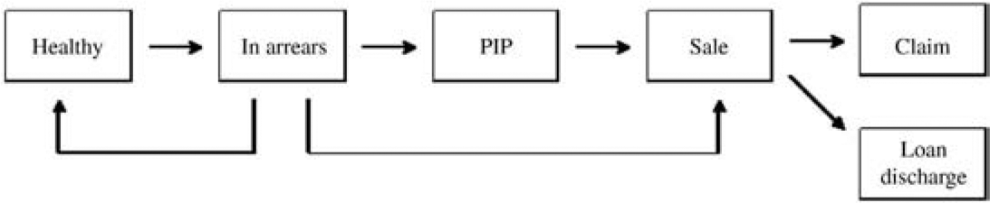
The transitions between loan statuses leading to a claim are represented in Figure 1. The figure also includes two additional transitions not covered by the description above. These reflect the facts that

• Many cases of arrears are cured (returned to healthy status);

• Some borrowers in arrears voluntarily undertake sale and thus bypass the PIP status.

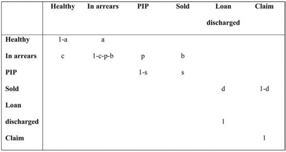
Many transitions proceed directly from healthy to sale, but these lie outside the arrears/claim model. They result in policy terminations, discussed in Section 6.2, and also affect the exposures to transition, taken into account in Equation (3.4). The transition matrix associated with this process has the appearance set out in Figure 2.

Note that “Loan discharged” and “Claim” are absorbing states, and the set of states {PIP, Sold, Loan discharged, Claim} is absorbing.

This type of cascaded model involving the transition of individuals between certain states, which will later be assumed a Markov chain, is of growing prominence in the actuarial literature. A few examples from the literature are G. C. Taylor (1971), Haberman and Pitacco (1999), Jones (1997), and G. Taylor and Campbell (2002).

2.2. Date of claim occurrence

The usual definition of the date of occurrence of a claim is the date of the event generating the claim. In the case of mortgage insurance, there is some ambiguity about this date.

Past papers have tended to treat it as the date on which the sale of the property occurred and proceeds were found to be insufficient; i.e., that date on which the existence of the claim became known with certainty. An alternative school of thought might maintain that the event generating the claim was the policy’s transition to the arrears status.

The choice of date of occurrence may affect the evaluation of an insurer’s technical liabilities. These consist of the outstanding claims liability and the unexpired risk liability, which may in turn be expressed as

• The liability for incurred but not paid (IBNP) claims, conventionally referred to as outstanding claims; and

• The liability for written but not incurred (WBNI) claims (unexpired risk).

Note that incurred but not reported (IBNR) claims form a segment within IBNP and refer to those claims that have “occurred,” in whatever sense has been adopted, but whose occurrence has not been reported to the insurer (by the lender, for example).

A change to the definition of date of occurrence causes a change in the dissection of total technical liabilities into these two components. It does not affect the expected value of the total liability, but it may affect the provision made for it in the insurer’s account because the provision made for unexpired risk is often an unearned premium provision. If this is defined by reference to incidence of risk, as mentioned in Section 1, it will take the value

$$P\left\{1-\mathrm{E}\left[C_{t}\right] / \mathrm{E}\left[C_{n}\right]\right\} \tag{2.1}$$

for a specific contract after t years of its n-year term have elapsed, where P is the premium payable under the contract net of acquisition and reinsurance expense, and C_t denotes the amount of claims incurred in the t years.

Let this quantity be denoted U_t. Then

$$\begin{aligned} U_{t} & =P / \mathrm{E}\left[C_{n}\right]\left\{\mathrm{E}\left[C_{n}\right]-\mathrm{E}\left[C_{t}\right]\right\} \\ & =(1+\pi)\left\{\mathrm{E}\left[C_{n}\right]-\mathrm{E}\left[C_{t}\right]\right\}, \end{aligned} \tag{2.2}$$

where the term within braces is the expected WBNI claims, and π is the profit margin contained in P expressed as a proportion of risk premium.

Thus unearned premium reserves include not only the relevant expected claim cost but also the associated profit margin. If this margin is positive, the unearned premium will exceed the expected claim cost. It follows that the later the choice of date of claim occurrence in Figure 1, the greater will be the estimated total amount of technical liabilities.

3. Model structure

The present section describes the model used to represent the claims process of Section 2.

3.1. Cascaded model

Figure 2 suggests a model consisting of a cascade of submodels, with each submodel representing a single transition. The resulting models are as follows:

1. Submodel 1: Probability of transition from healthy to in arrears.

2. Submodel 2: Probability of cure of arrears.

3. Submodel 3: Probability of transition from arrears to PIP.

4. Submodel 4: Probability of transition from PIP to sold.

5. Submodel 5: Probability of transition from sold to claim.

6. Submodel 6: Distribution of claim sizes.

This is a slightly abbreviated version of the model suggested by Figure 2, which omits the model of transition from in arrears to sold. This case has, in fact, been recognized by the insertion of an artificial transition to PIP infinitesimally prior to the sale. More accurately, therefore, Submodels 3 and 4 are as follows:

1. Submodel 3: Probability of transition from arrears to PIP or sold.

2. Submodel 4: Probability of transition from PIP to sold, with infinitesimal duration between the two indicating a direct transition from in arrears to sold.

The cascaded model is assumed to be Markovian.

3.2. Submodel structures

3.2.1. Submodels 1 to 5

Each of Submodels 1 to 5 consists of a collection of binomial variates observed over calendar intervals j = 1, 2, . . . , J. These intervals are of equal but arbitrary length. We have found quarterly intervals useful. The variates are

$$Y_{i j}^{(m)} \sim \operatorname{Bin}\left[1,1-\exp \left\{u_{i j}^{(m)} \log \left[1-p_{i j}^{(m)}\right]\right\}\right], \tag{3.1}$$

where Y_ij^(m) denotes the binomial response of the i-th policy in Submodel m (= 1, . . . , 5) over the j-th interval, p_ij^(m) the associated probability of transition, and u_ij^(m) the amount of time the policy is at risk of transition.

Note the use throughout of the superscript m to indicate that Submodel m is under discussion. In particular, p_ij^(m) does not denote an m-step transition probability, as this notation often does.

The quantities u_ij^(m) take values in the range [0,1]. Values less than unity recognize incomplete intervals of exposure. For example, a loan that commences in an interval will be at risk of transition to arrears only for the remainder of that interval; likewise, a policy that terminates will be at risk of transition only for a fraction of the interval.

In general, if the interval j denotes [j, j + 1] and p_ij^(m) relates to transition from status s₁ to s₂, then

$$u_{i j}^{(m)}=t_{2}-t_{1}, \tag{3.2}$$

where

$$t_{1}=\max \left(j, \text { date first in status } s_{1} \text { in interval } j\right) \tag{3.3}$$

$$\begin{aligned} t_{2} &= j + 1, \text{ if transition to } s_{2} \text{ occurs during the interval}\\ & = \min (j+1, \text{ date of termination of the policy}), \text{ otherwise.} \end{aligned}\tag{3.4}$$

The notation above implicitly assumes that only one transition s₁ → s₂ can occur in a single interval. In fact, multiple transitions may occur when the status is healthy or in arrears. To accommodate this within the notation is unnecessarily cumbersome. The notation is therefore left as above, and its extension to multiple transitions within an interval is taken as obvious.

A transition probability defined in this way is the probability that the transition in question would occur over a complete quarter if no other transition intensities were operating. In actuarial terminology, it is an independent transition probability (Benjamin and Haycocks 1970).

The probabilities in Equation (3.1) may be naturally represented as

$$\operatorname{logit} p_{i j}^{(m)}=\Sigma_{k} \beta_{k}^{(m)} x_{i j k}, \tag{3.5}$$

where x_ijk denotes value for observation (i, j) of the k-th predictor used in the six submodels (any one predictor may be used in more than one model, but not necessarily in all), and β_k^(m) its associated coefficient.

Each model consisting of Equations (3.1) and (3.5) is a generalized linear model (GLM) (McCullagh and Nelder 1989).

3.2.2. Submodel 6

The response variable Y_ij⁽⁶⁾ is continuous, but it may also be modeled with a GLM:

$$Y_{i j}^{(6)} \sim \operatorname{EDF}\left(\mu_{i j}, q\right) \tag{3.6}$$

$$\log \mu_{i j}=\Sigma_{k} \beta_{k}^{(6)} x_{i j k}, \tag{3.7}$$

where EDF(μ_ij,q) denotes a member of the exponential dispersion family with

$$\mathrm{E}\left[Y_{i j}^{(6)}\right]=\mu_{i j} \tag{3.8}$$

$$\operatorname{Var}\left[Y_{i j}^{(6)}\right]=\left(\varphi / w_{i j}\right) \mu_{i j}^{q} \tag{3.9}$$

for constants ϕ, w_ij.

For any given i, there can, of course, be only one observation Y_ij⁽⁶⁾; i.e., for a unique j. The index j has been retained in the model because of the possible dependency of the predictors x_ijk on it. Further comment on this appears in Section 3.3.

3.3. Predictors

The predictors x_ijk fall into three categories, which may be briefly designated:

• Policy variables, with subcategories

  • Static,

  • Dynamic,

• External variables,

• Manufactured risk indicators.

A reasonably comprehensive list of predictors appears in Section 4.1.

Policy variables assume values that are specific to individual policies; e.g., date of policy issue, loan-to-valuation ratio (LVR), etc. Static variables are those whose values remain constant over time (the two examples just given), while dynamic variables change over time (e.g., for a policy in arrears, number of quarters since transition to that status).

Some dynamic variables, such as this last one, will be simple mappings of calendar time (transition quarter); hence, the retention of the index j in the notation Y_ij⁽⁶⁾, on which comment was made at the end of Section 3.2.

External variables are external to individual policies and assume values that apply globally over all policies. They are indicators of the external economy, such as housing prices, interest rates, etc.

Manufactured risk indicators are specifically constructed from other variables as indicators of the risks inherent in specific submodels. Examples of these are updated debt servicing ratio (DSR) and potential claim size, defined as follows:

$$\text { Updated DSR }=\frac{\begin{array}{c} \text { Current outstanding principal } \\ \times \text { interest rate } \end{array}}{\begin{array}{c} \text { Borrower's annual income } \\ \times \text { average earnings growth factor } \end{array}} \tag{3.10}$$

$$\begin{aligned} & \text{Potential claim size} =\\ & \quad \text{Amount of arrears}\\ & \quad \text{Less}\\ & \quad \text{Principal repaid}\\ & \quad \text{Less}\\ & \quad [\text{Housing price growth factor} \times(1-q)-1 ]\\ & \quad \times\\ & \quad \text{Original loan amount/LVR,} \end{aligned}\tag{3.11}$$

where

• the borrower’s annual gross income is the amount indicated when the loan was issued (which is the latest that will usually be on file);

• the average earnings and housing price growth factors are external variables, and relate to the period from inception of the loan to the current date;

• q is the proportion of property value lost in deadweight costs on sale.

If original DSR is defined as the ratio of the borrower’s original per-period interest commitment to annual income, an obvious indicator of the likelihood of arrears, then updated DSR is a revised version allowing for any reduction of principal, change in interest rate, and change in income over the course of the loan to date.

Potential claim size comprises three members, of which the last two provide an estimate of the borrower’s current equity in the property less the costs of realizing it. The total quantity (3.11) is therefore an estimate of the amount of loss that would arise in the event of a claim.

4. Forecasting expected claim cost

4.1. Model fitting

The present section describes the fitting of the model of Section 3 to observations on loans and their transitions between states.

4.1.1. Data

The fitting of the six models described in Section 3.2 relied on two datasets:

• A policy file, containing one record per policy issued by the insurer over a period of years, and each record containing various attributes of the policy that are used as policy variable predictors described in Section 3.3.

• An arrears file, containing one record per occurrence of arrears i.e., transition of a loan from a healthy status to in arrears, and each record containing details of the arrears, including its progress through the statuses illustrated in Figure 1, particularly the dates of each transition.

Unfortunately, the proprietary nature of the data has prevented us from providing more detail.

4.1.2. Modeling

Since the six submodels are GLMs, they may be fitted to the data by means of GLM software. This may be computationally intensive. For example, in the case of an insurer with about 1.25 million policies in force, Model 1 involved about 23 million observations (i.e., (i, j) combinations), one for each quarter that each policy characterized as “healthy” (i.e., at risk of transition to arrears) was in force over a nine-year experience period (including policies no longer in force).

Otherwise, the application of the software is routine, with one exception. The appearance of the term u_ij^(m) in (3.1) creates some awkwardness. However, substitution of Equation (3.5) into the probability in Equation (3.1), followed by a logit transform, yields (with suffixes temporarily suppressed for brevity)

$$\operatorname{logit}(1-\exp u \log (1-p))=\operatorname{logit}\left[1-\left(1+e^{\eta}\right)^{-u}\right], \tag{4.1}$$

where η denotes the linear predictor of the model; i.e., the right side of Equation (3.5).

A little manipulation produces

$$\begin{aligned} \operatorname{logit} & (1-\exp u \log (1-p)) \\ = & \log \left[\left(1+e^{\eta}\right)^{u}-1\right] \\ = & \log u+\eta+(1 / 2)(u-1) e^{\eta} \\ & \left.+(1 / 24)(u-1)(u-5) e^{2 \eta}+\cdots\right] \end{aligned} \tag{4.2}$$

where (1 + e^η)^u has been expanded as a power series in e^η, and the logarithmic function has then been expanded as a power series.

This shows that the logit transform of the probability in (3.1) may be represented by (3.5) with a correction term of logu, subject to an error of O(½(u − 1)e^η) = O(½(u − 1)p/(1 − p)). The error is thus small for p → 0 or u → 1. In GLM terminology, the correction term amounts to adding an offset of log u into the model.

This treatment of fractional exposures within a discrete-time framework is somewhat cumbersome but, as explained earlier in this section, the modeling involves a large dataset, and we are unaware of continuous-time software that would be equal to the task.

In mitigation, it might be pointed out that the observations involving fractional exposures relate mainly to transitions between statuses (which usually occur within a calendar period) and therefore form a distinct minority of the whole set of observations. Any distortion caused by the truncation of (4.2) should therefore be modest.

For Model 6, the value q = 1.5 was found to be satisfactory in (3.9). This means that the distribution of claim size is skewed to the right but shorter tailed than gamma.

For reasons of confidentiality (not to mention space), full numerical results are not presented here. However, a couple of examples will be useful.

Example 1. Model of claim size

One of the strong predictors of average claim size is the potential claim size defined in (3.11). It contributes to the linear predictor (3.7) as follows:

$$0.71 \times \log [\text { Potential claim size } / 1000+5] .$$

In view of the model’s log link, this means that forecast claim size is proportional to [Potential claim size/1000 + 5]^0.71; and so, for example, PIP cases with potential claim sizes of $20,000 and $5,000, respectively, but otherwise identical, will have forecast claim sizes in the ratio 1.9:1.

Example 2. Model of transition from healthy to in arrears

The probability of transition from a healthy status to in arrears is found to depend on duration from commencement of the loan, after allowance has been made for all other predictors. In fact, this probability decreases with increasing development quarter (defined as the difference between the calendar quarter of commencement of the loan and the quarter of transition). From development quarter 1 onward, the decrease is linear.

Table 1 displays the predictors estimated to have statistically significant regression coefficients β in the six models. Table 2 provides some interpretive comment on some of the predictors.

Many of the issues involved in fitting the model of claims experience are the same as for GLM loss reserving in any other line of business (see, e.g., G. Taylor and McGuire 2004).

For example, in each of the submodels of transition from a source status to a target status, one has the choice of the following time-based predictors:

• issue quarter,

• duration since transition into the source status, or

• transition quarter.

These three time dimensions correspond to accident quarter, development quarter, and calendar quarter in a more conventional loss reserving. As usual, collinearity is likely to prevent efficient inclusion of all three in a model, even if all three have some predictive power. In this case, it will be desirable to apply a little effort to determining which two have the greatest predictive power.

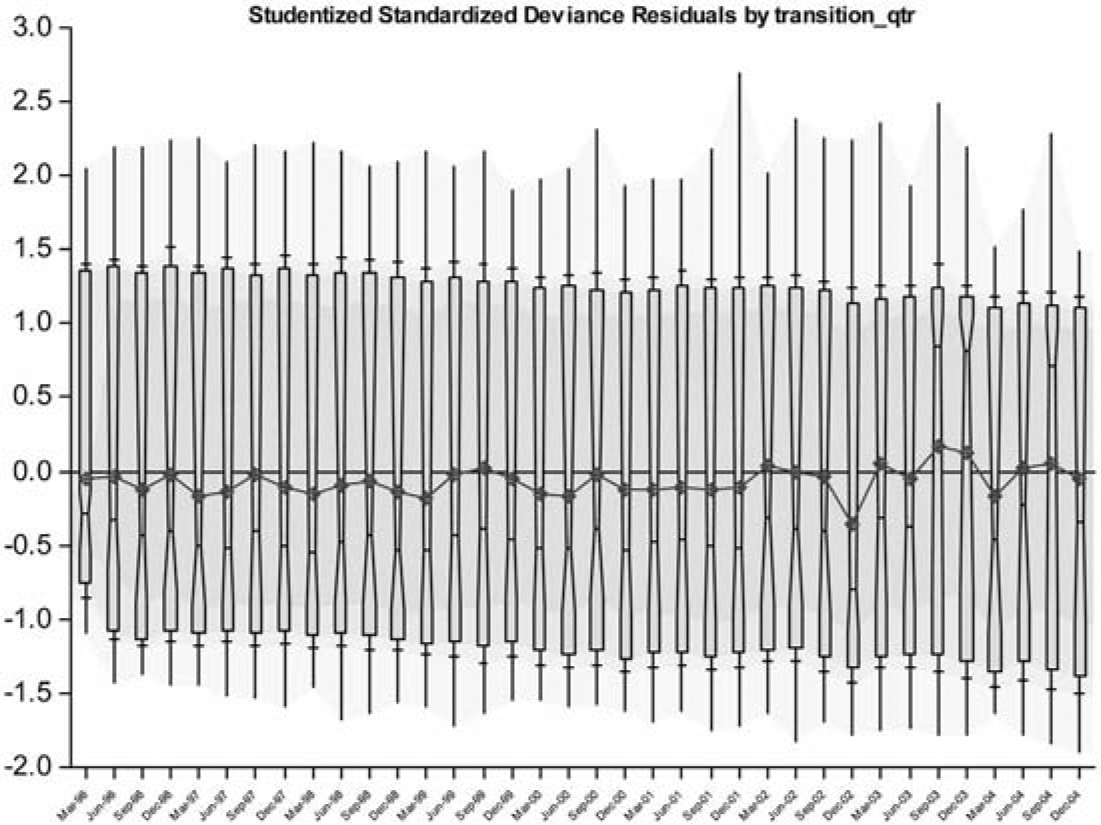
It is also desirable to examine the usual diagnostics of a GLM regression, such as residual plots, and triangles of observed to fitted value ratios by “accident period” and “development period.” Figure 3 provides an example of the former in respect of Submodel 2, the probability of cure of arrears.

In this figure,

• the boxes represent the interquartile ranges;

• the marked points joined by the broken line are the means,

• the whiskers indicate the total range of observations, and

• the horizontal bars on the whiskers mark the 10th and 90th percentiles.

The figure indicates centeredness and homoscedasticity of the residuals with respect to transition quarter.

Forecasts of the external variables will be required. It will usually be desirable that these be obtained from a separate econometric model, which might include housing prices, stock prices, gross domestic product, interest rates, inflation rates, unemployment rates, and possibly other variables.

4.2. Forecast claims experience

The conventional form of forecast in a loss reserve model consists of plugging future values of the predictors, such as accident period and development period, into the calibrated model and taking the results as forecasts of future claim cash flows.

There are two reasons why this is neither feasible nor reliable on the present occasion:

• Such treatment of a cascaded model is unlikely to be computationally feasible.

• For specific reasons related to mortgage insurance, it is likely to produce a biased forecast.

4.2.1. Cascaded models

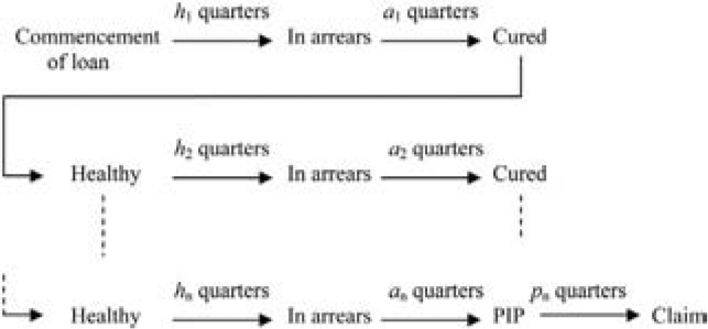
Note from Table 1 that Submodels 1, 2, and 3 all include “development quarter” (in the form of one or more of duration since issue, duration since arrears, and duration since PIP, respectively) as a predictor. Figure 4 illustrates the typical evolution of a claim.

The probability of this occurrence is equal to the compound of (h₁ + a₁) + · · · + (h_n + a_n) + p_n single quarter probabilities, where h₁, a₁, . . . , h_n, a_n, p_n, and even n itself, are random variables. There are thus many combinations of single quarter probabilities, too many for feasible computation.

It is necessary, therefore, to simulate the experience of each policy in force at a valuation date. The simulated liability in respect of each policy will then be a random variable instead of the expected liability, but by the law of large numbers, the realization of the liability for a large number of policies will approximate its expected value.

The simulation will yield the forecast information set out in Table 3.

4.2.2. Multistep transitions

The simulation of claims experience is not without complexities because, as was pointed out in Section 3.2, multistep transitions can occur within a single quarter. Table 3 indicates that statuses are recorded only at the end of a quarter, but the transition between end-quarter statuses for consecutive quarters may be multi-step.

For example, the status may be healthy at the ends of both quarters q and q + 1, but there may have been any number of healthy→in arrears→healthy cycles within the quarter.

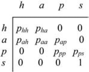
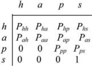
These difficulties arise as a direct result of modeling an essentially continuous-time process in a discrete-time framework, the reason for which was given in Section 4.1. Treatment of the matter requires a continuous-time formulation of the discrete Markov process described by Figure 2, as abbreviated in Section 3.1. The discrete-time transition matrix for the abbreviated process is displayed in Figure 5, and its continuous-time equivalent in Figure 6.

In these matrices, the statuses of healthy, in arrears, PIP, and sold are denoted by h, a, p, and s, respectively. The claim status is omitted, because the transition into it from sold is not time dependent, but is a simple probability.

The quantity λ_rs (s ≠ t) denotes the intensity of status transition r → s between the end of quarter t and the end of quarter t + 1 (assumed constant over this interval) and, since p_rs is an independent transition probability (see Section 3.2),

$$\lambda_{r s}=-\log \left(1-p_{r s}\right) \tag{4.3}$$

Table 3 requires the quantities

$$\begin{array}{c} P_{r s}=\operatorname{Prob}[\text { status } s \text { at end of quarter } t+1 \mid \\ \text { status } r \text { at end of quarter } t] \end{array} \tag{4.4}$$

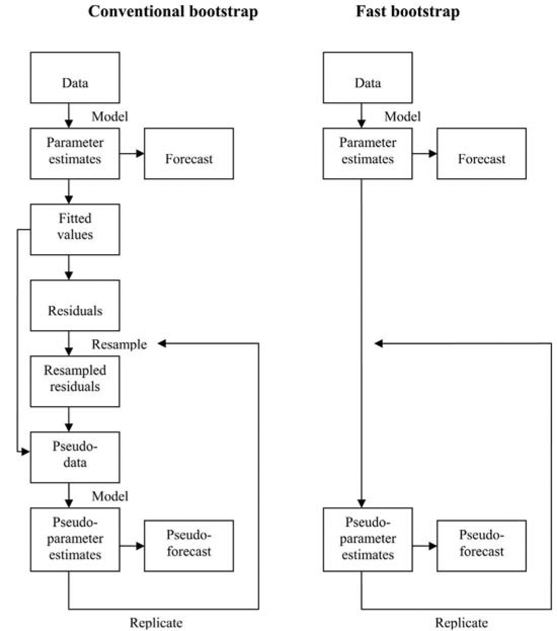
It is evident that the “whole quarter” transition matrix takes the form set out in Figure 7.

Consider the interval of time between the end of quarter t and the end of quarter t + 1 and let the time elapsed since t be denoted by α where 0 ≤ α ≤₁. Define

$$\begin{array}{r} P_{r s}(\alpha)=\operatorname{Prob}[\text { status } s \text { at } \alpha \mid \text { status } r \\ \text { at end of quarter } t] \end{array} \tag{4.5}$$

Then P_rs(1) = P_rs as defined in (4.4).

Values of P_rs(1) were calculated by solving the Kolmogorov Forward Equation

$$\partial W(\alpha) /\left.\partial \alpha\right|_{\alpha=1}=W(\alpha) Q, \tag{4.6}$$

subject to initial conditions W(0), where W(α) is the partial quarter transition matrix and Q is the continuous-time transition matrix (Figure 6). The Kolmogorov Forward Equation was solved using Mathematica (n.d.), and the values of P_rs(1) are set out in Appendix A. These are the probabilities used to simulate change in status from one quarter-end to the next.

If policy m attains end-quarter status s for the first time in quarter j*, the further transition to either claim or discharged status is simulated. If the latter, simulation for the policy is terminated; if status is claim, a claim size Y is simulated from Submodel 6, as described in Appendix B, and then simulation for the policy is terminated. In the case of discharge, Y is set to zero.

Let L_i^(j) denote claim payments for policy i in quarter j. Then the simulated value is

$$\begin{aligned} L_{i}^{(j)} & =Y, & & \text { for } \quad j=j^{*} \\ & =0, & & \text { otherwise } . \end{aligned} \tag{4.7}$$

The total liability for future claims is then

$$L=\sum_{i, j} L_{i}^{(j)} \tag{4.8}$$

where the summation runs over all values of i and future values of j. The total liability can be dissected in any way required (e.g., according to year of policy issue) simply by summing over subsets of (i, j) in (4.8).

4.2.3. Stochastic future parameters

There is a second reason why simulation may be a desirable form of loss reserving. Let

$$\begin{array}{c} L_{. i}=\sum_{j} L_{i}^{(j)}=\text { simulated liability in respect of } \\ \text { policy } i \end{array} \tag{4.9}$$

$$L_{j .}=\sum_{i} L_{i}^{(j)}=\underset{\text { respect of calendar quarter } j}{\text { simulated liability cash flow in }} \tag{4.10}$$

so that

$$L=\sum_{i} L_{. i}=\sum_{j} L_{j} \tag{4.11}$$

The forecast of L_j. will depend on the estimates $\hat{\beta}_k^{(m)}$ of the model parameters $\beta_k^{(m)}$, m = 1, . . . , 6, and also on the x*_ijk taken in future quarter j by the predictors x_ijk. With these dependencies made explicit, (4.8) suggests the forecast

$$L^{*}=\sum_{i, j} L_{i}^{(j)}\left(\hat{\beta}, x_{i j}^{*}\right) \tag{4.12}$$

where $\hat{\beta}$ is the vector of values $\hat{\beta}_k^{(m)}$ over all m, and x*_ij the vector with components x*_ijk.

In the terminology of Section 3.3, x*_ij may be decomposed into subvectors:

$$x_{i j}^{* T}=\left[\xi_{i}^{* T}, \zeta_{i j}^{* T}, z_{i j}^{* T}\right], \tag{4.13}$$

where ξ*_i contains static policy variables (which do not depend on j), ζ*^T_ij contains dynamic policy variables, z*^T_ij contains forecasts of external variables and manufactured risk variables, and T denotes the operation of transposition.

Dynamic policy variables depend on j but are simple mappings of it (e.g., number of quarters since transition to in arrears status), whereas external variables and manufactured risk variables require forecast. Examples of such predictors, from Table 1, are growth in house price, growth in stock price, and generally any predictor taken from an economic time series.

The z*_ijk are forecasts of quantities z_ijk that may be viewed here as themselves random variables. In this case an unbiased forecast of L will be

$$L^{*}=\sum_{i, j} \mathrm{E}\left[L_{i}^{(j)}\left(\hat{\beta}, x_{i j}\right)\right]=\sum_{i, j} \mathrm{E}\left[L_{i}^{(j)}\left(\hat{\beta}, \xi_{i}^{*}, \zeta_{i j}^{*}, z_{i j}\right)\right] \tag{4.14}$$

Note that, in general, this is not equal to the alternative forecast

$$L^{\prime *}=\sum_{i, j} L_{i}^{(j)}\left(\hat{\beta}, \mathrm{E}\left[x_{i j}\right]\right)=\sum_{i, j} L_{i}^{(j)}\left(\hat{\beta}, \xi_{i}^{*}, \zeta_{i j}^{*}, \mathrm{E}\left[z_{i j}\right]\right) \tag{4.14a}$$

Indeed, Jensen’s inequality (see, e.g., Royden 1968) indicates that (4.14a) may be distinctly biased relative to (4.14).

Jensen’s inequality. Let A be a real interval and let f : A→R be convex in the sense that αf(x₁) + (1 − α)f(x₂) ≥ f(αx₁ + (1 − α)x₂) for all x₁,x₂ ∈ A and all 0 < α < 1. Let X be a random variable defined on A. Then

$$\mathrm{E}[f(X)] \geq f(\mathrm{E}[X]) \tag{4.15}$$

with equality if and only if either f is linear (i.e., equality in the definition of convexity) or the distribution of X is concentrated at a single point.

Note that a sufficient condition for f to be convex is that f″ ≥ 0.

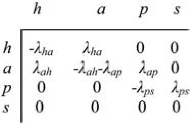
Now consider the functional dependency of L* on z_ij, a subvector of economic time-series variables, such as house price increases or stock price increases. The functional dependency on some of these quantities involves considerable convexity.

This is particularly the case for house price increases, whose influence on liability is illustrated by Figure 8. If z_ijk denotes future annual house price increase, then ∂²L/∂z²_ijk > 0, and Jensen’s inequality applies.

If other predictors are fixed at their expected values for the moment, then (4.15) yields

$$\mathrm{E}\left[L\left(\hat{\beta}, x_{i j}\right)\right] \geq L\left(\hat{\beta}, \xi_{i}^{*}, \zeta_{i j}^{*}, \mathrm{E}\left[z_{i j}\right]\right) \tag{4.16}$$

What this means is that estimating liability by taking mean forecasts of future house price increases and plugging them into a liability formula as if they were certain will inevitably underestimate. The extent of the underestimation will increase with

• the convexity of the liability with respect to future house price growth, and

• the dispersion of the distribution of these increases.

If the liability displays the same sort of convexity with respect to other predictors x_ijk, the failure of the “plug-in” approach to predictors of the future economic time-series type will be even greater. This sort of result has recently been observed empirically by Kelly and Smith (2005).

This feature of loss reserving is virtually unique to mortgage insurance. The forecasting of liability in other lines of business does not usually depend heavily on future economic time series. The main exception to this is future claims for inflation, but commonly the convexity of liability with respect to this variable is less than its mortgage insurance counterpart, and the dispersion in the future time series will often be less than in mortgage insurance.

The estimation of liability by means of simulation avoids this form of underestimation. The future values of z_ij are simulated from a model of the external economic influences. It is likely that the components z_ijk will not all be independent. In any case, let z_ij^(r), r = 1, . . . ,R, denote the r-th simulated replicate.

Then, by (4.14), an unbiased forecast of L is

$$L^{*}=R^{-1} \sum_{i, j, r} \mathrm{E}\left[L_{i}^{(j)}\left(\hat{\beta}, \xi_{i}^{*}, \zeta_{i j}^{*}, z_{i j}^{(r)}\right)\right] \tag{4.17}$$

The computation in (4.17) is substantial. It involves R simulations of the future experience of each policy i over future quarters j, with different replicates of external economic variables in each of the R simulations.

5. Forecast error

The present section describes the estimation of the standard errors associated with the various predictions of the model.

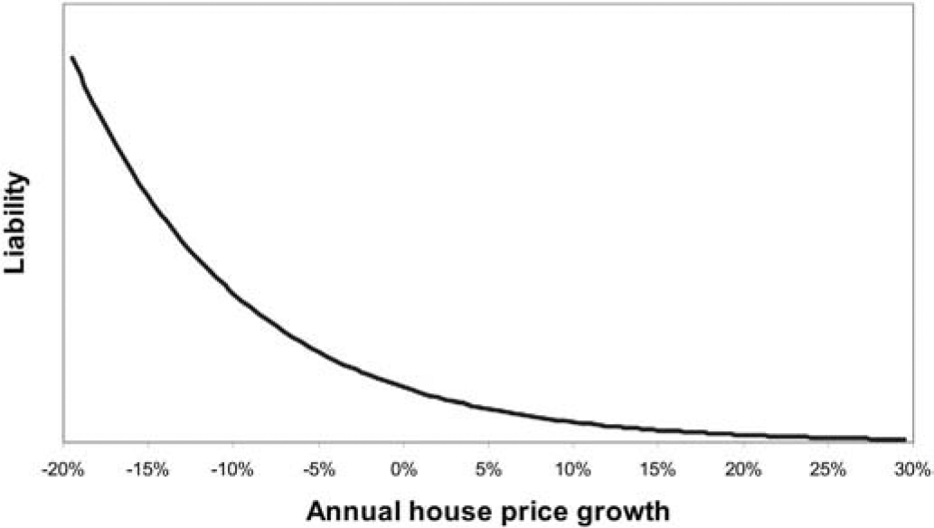
5.1. Fast bootstrap

Estimation of the forecast error contained in L* for such a complex model as defined in Section 3 will not be feasible other than by some form of bootstrap. However, the conventional form of bootstrapping, with the refitting of the six models to each pseudo-data set is not likely to be feasible.

A “fast bootstrap,” such as discussed in Section 8.3 of England and Verrall (2002), has therefore been used, in which the steps of generating pseudo-data sets and refitting the model to them have been bypassed. Instead, pseudo-estimates of the model parameters are obtained simply by perturbing the original estimates, with due reference to their standard errors.

More precisely, the procedure is as follows. It is supposed that the vector of parameter estimates β̂ is accompanied by an estimate V of the associated covariance matrix. The standard GLM software packages (SAS GENMOD, Emblem, etc.) produce this.

If β denotes the vector of parameters estimated by β̂ (let its dimension be q), suppose that

$$\hat{\beta} \sim N(\beta, V) . \tag{5.1}$$

This is asymptotically true for large samples for the maximum likelihood estimate β̂. It is not to assume, of course, that the observations Y_ij^(m) are normally distributed.

Diagonalize V:

$$V=P^{T} D P \tag{5.2}$$

where D is diagonal and P is orthogonal. Then

$$P \hat{\beta} \sim N(P \beta, D) \tag{5.3}$$

Thus, the components of Pβ̂ may be sampled independently. Let ε⁽ⁿ⁾, n = 1, . . . ,N, be a q-vector of samplings from the unit normal distribution, and define

$$\hat{\beta}^{(n)}=P^{T}\left(P \hat{\beta}+D \varepsilon^{(n)}\right)=\hat{\beta}+P^{T} D \varepsilon^{(n)} . \tag{5.4}$$

Then the $\hat{\beta}^{(n)}$ are replicates of $\hat{\beta}$ in the sense of satisfying (5.1). These generate replicates L*⁽ⁿ⁾ of L* whose dispersion reflects the parameter error in the forecast L*; i.e., the uncertainty in L* induced by uncertainty in β̂ . Note that this is computationally demanding, requiring N replicates of the previous R simulations.

Figure 9 compares the fast bootstrap procedure with the conventional one, illustrating how the former omits the data resampling steps.

5.2. Estimation of forecast error

The fast bootstrap of Section 5.1 is applied as follows.

5.2.1. Components of forecast error

Consider the forecast L* in (4.17). Let L denote the true (yet to be observed) value of the liability. The forecast error is

$$\Delta=L-L^{*} . \tag{5.5}$$

Noting that L* = E[L | β̂], one may decompose this expression as follows:

$$\Delta=\{L-\mathrm{E}[L]\}-\{\mathrm{E}[L \mid \hat{\beta}]-\mathrm{E}[L]\} .$$

This expression may be decomposed further:

$$\begin{aligned} \Delta= & \{L-\mathrm{E}[L]\}-\{\mathrm{E}[L \mid \mathcal{M}, \hat{\beta}]-\mathrm{E}[L \mid \mathcal{M}]\} \\ & -\{\mathrm{E}[L \mid \mathcal{M}]-\mathrm{E}[L]\} \\ = & \Delta_{\text {Proc }}-\Delta_{\mathrm{Pa}}-\Delta_{\mathrm{Sp}}, \quad \text { say } \end{aligned} \tag{5.6}$$

where E[L | β̂] has simply been rewritten as E[L | M,β̂], recognizing the model structure to which the parameter estimates β̂ belong.

The three terms on the right side of (5.6) may be recognized as process error, parameter error, and model specification error in the standard terminology. In fact, it is useful to decompose the second of these even further:

$$\begin{aligned} \Delta_{\mathrm{Pa}}= & \mathrm{E}[L \mid \mathcal{M}, \hat{\beta}]-\mathrm{E}[L \mid \mathcal{M}] \\ = & \left\{\mathrm{E}[L \mid \mathcal{M}, \hat{\beta}]-\mathrm{E}\left[L \mid \mathcal{M}, \hat{\beta},\left\{x_{i j}\right\}\right]\right\} \\ & +\left\{\mathrm{E}\left[L \mid \mathcal{M}, \hat{\beta},\left\{x_{i j}\right\}\right]-\mathrm{E}[L \mid \mathcal{M}]\right\} \\ = & \Delta_{\text {Pred }}+\Delta_{\text {Par }}, \text { say } \end{aligned} \tag{5.7}$$

where {x_ij} denotes the set of predictors over all i, j, and so (5.7) decomposes parameter error into that due to variation in the parameters β, and that due to variation in the predictors.

Recall from Section 4.2 that that x_ij consists of ξ_i, ζ_ij and z_ij, of which the first two are non-random (other than captured in process error), so Δ_Pred and Δ_Par could equally well be defined with {z_ij} written in place of {x_ij}.

By (5.6) and (5.7),

$$\Delta=\Delta_{\text {Proc }}-\left[\Delta_{\text {Pred }}+\Delta_{\text {Par }}\right]-\Delta_{\mathrm{Sp}} . \tag{5.8}$$

The four members on the right are stochastically independent, and so the mean square error of prediction is

$$\begin{aligned} \operatorname{MSEP}[L]= & \operatorname{Var}\left[\Delta_{\text {Proc }}\right]+\operatorname{Var}\left[\Delta_{\text {Pred }}\right] \\ & +\operatorname{Var}\left[\Delta_{\text {Par }}\right]+\operatorname{Var}\left[\Delta_{\text {Sp }}\right] \end{aligned} \tag{5.9}$$

5.2.2. Estimation

As usual, estimation of model specification error is problematic. It falls outside the scope of the statistical modeling considered here and, while an issue of substance, is not discussed further in this paper.

The other three components of forecast error can be estimated from the simulations defined in Section 4.2. This will require multiple replicates of the forecast (4.17). The details are given in Appendix C.

6. Miscellaneous other matters

There are a couple of matters of relevance to mortgage insurance reserving that are not integral to the modelling described above. They are discussed in the following subsections.

6.1. Earning of premium

Section 1 notes the typical requirement that premium be earned over the term of a policy in proportion to the expected claim cost incurred.

For policies with inception quarter J, define the earning pattern over quarters J, J + 1, J + 2, . . . to be the vector of expected claims incurred in those quarters expressed as a proportion of the total incurred for those policies. Denote the proportion associated with quarter J + d by π_d^(J), where d will be referred to as development quarter.

Estimation of the earning pattern will require a definition of when claims are incurred. In general, a claim is incurred at the time of occurrence of the event causing it. However, in mortgage insurance the definition of this event is less obvious than in other lines of business. It may reasonably be taken as the PIP event (or sale in the case that this is voluntary), or the commencement of the arrears leading to the claim. Other definitions may be possible.

For a policy i with inception quarter J, having completed D development quarters at a valuation date, an estimate of future claim payments L_i^(J+d), d = D + 1, D + 2, etc., is given by (4.10). Actual claim payments will be available for past development quarters d = 0, 1, . . . ,D. For present purposes, let these be denoted by L_i^(J+d) also.

This gives a complete vector of claim payments {L_i^(J+d),d = 0, 1, 2, . . .} for policies from inception quarter J. If an earning pattern is to be estimated, it will be necessary to recast these payments according to their dates incurred rather than dates paid.

If, for example, date incurred is taken as the PIP event, then all payments will need to be reassigned from payment quarter to PIP quarter. For past payments, these dates will be factual. For forecast future payments, there will be simulated PIP and payment quarters, according to which the reassignment may be made.

This reassignment will convert the payment vector {L_i^(J+d),d = 0,1,2, . . .} to a vector of incurred amounts {I_i^(J+d),d = 0,1,2, . . .} where

$$\Sigma_{d} L_{i}^{(J+d)}=\Sigma_{d} I_{i}^{(J+d)} \tag{6.1}$$

The earning pattern may now be calculated as

$$\pi_{d}^{(J)}=I^{(J+d)} / \Sigma_{d} I^{(J+d)}, \quad d=0,1,2, \text { etc. }, \tag{6.2}$$

where

$$I^{(J+d)}=\sum_{i} I_{i}^{(J+d)} \tag{6.3}$$

the summation over i running over all policies with inception quarter J.

Note that the notation π_d^(J) expresses dependency on J. This dependency is induced by changes in the mix of policies (i.e., changing distribution of policy variables) with changing inception quarter and by changes in the economy (i.e., changing external variables) over time.

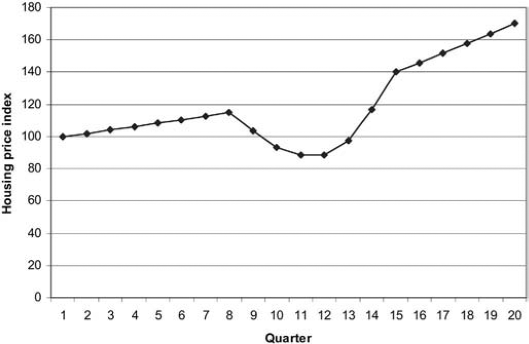
Consider, for example, the case represented in Figure 10, in which the housing market proceeds steadily over quarters 1 to 8, then crashes over the following four quarters, then recovers strongly.

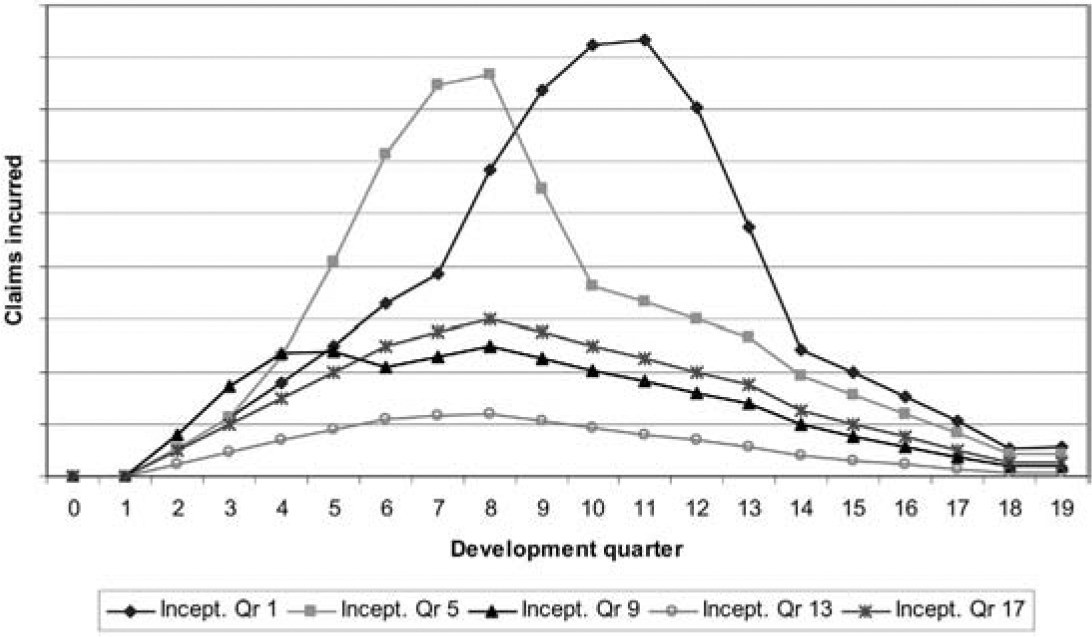
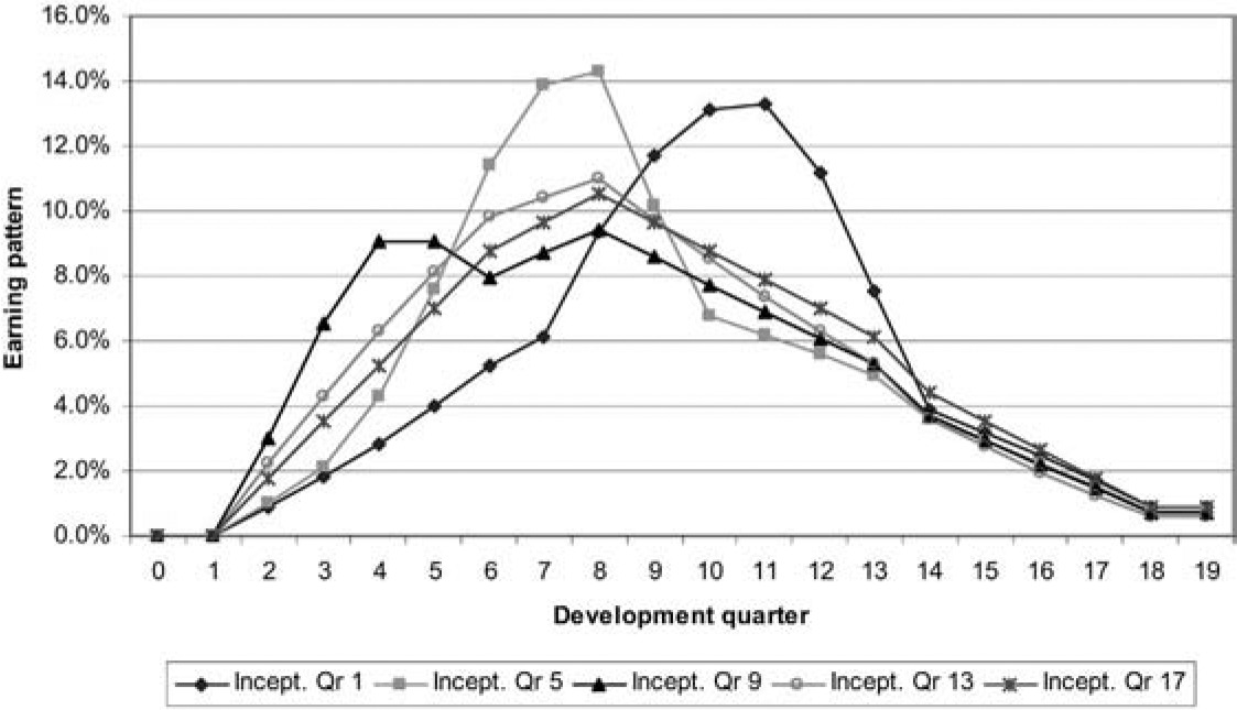
Figure 11 illustrates how claims might be incurred over time for a number of inception quarters, and Figure 12 converts these into earning patterns.

Inception quarter 17 experiences a steady 4% per quarter growth in house prices and may be taken as the standard in interpreting these plots.

Note that inception quarter 13 experiences a much lower level of claims. This is because the recovery in housing prices, with high growth rates, almost coincides with that quarter. As a result, housing prices have increased by 50% after four development quarters, compared with 17% for inception quarter 17. The corresponding increases after eight development quarters are 75% and 32%.

Inception quarters 1 and 5 have similar expected claims experiences except that the latter is displaced to the left. This is because the property price collapse affects it four development quarters earlier. Both of these inception quarters are associated with relatively heavy claims experience, also due to the collapse.

The earning patterns in Figure 12 simply reproduce Figure 11 but with each inception quarter rescaled to total 100%. This leads to slightly paradoxical results, such as the fact that premium for inception quarter 13 is earned considerably more slowly over the early development quarters than for inception quarter 9 (see Figure 13), despite the fact that the claims experience of the former is much lower and therefore the profit margin much higher.

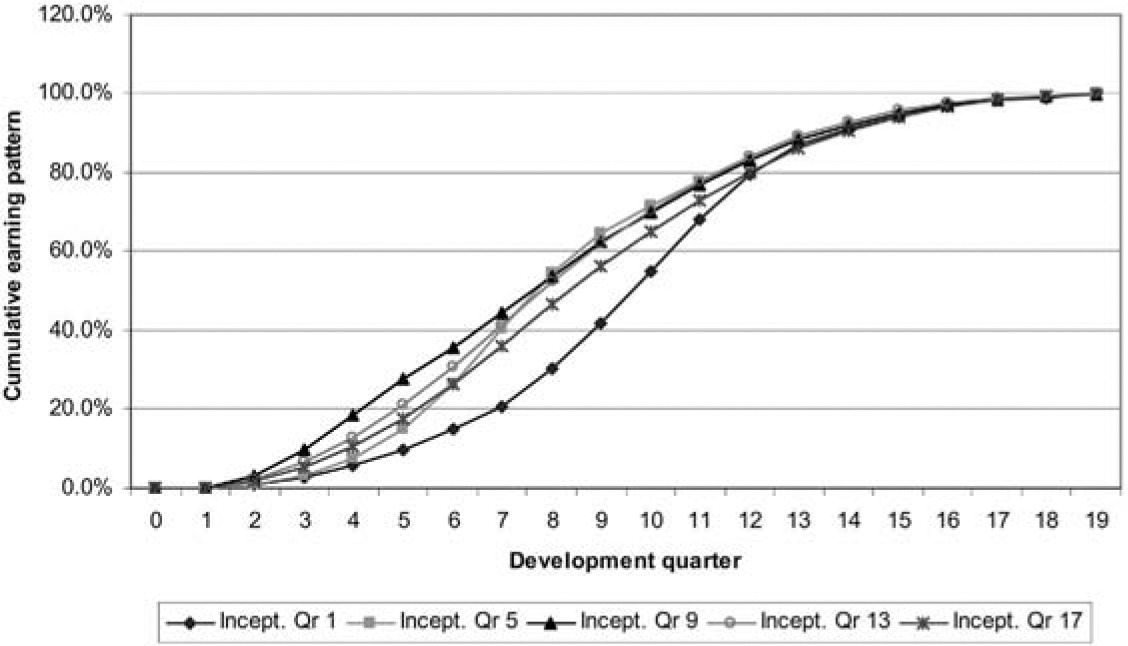
Of course, although the earning pattern for inception quarter 13 releases lesser percentages of the profit margin than in the case of inception quarter 9, the quantum of profit margin is much greater in the former case if there has been no change in premium rates.

6.2. Policy termination

It is common for mortgage insurance policies to be terminated before their term has elapsed. This usually occurs because the property is sold or the loan otherwise repaid before the term of the loan has expired.

It is necessary to allow for this form of exit from experience in calibrating Models 1 to 5 of Section 3.1. Specifically, in Equation (3.1) policy i must be assigned u_ij^(m) = fraction of calendar quarter j up to policy termination, when termination occurs in that quarter.

This ensures correct estimation of transition probabilities. However, there is a further question as to whether or not a valuation of technical liabilities should anticipate future terminations. In Australia, at least, it is typical for terminations not to attract any premium refund after one year’s policy duration. This means that underestimation of termination rates (such as not anticipating any) will lead to a conservative valuation.

The action taken in this area will be a matter of taste or statute or both. In the event that policy terminations are to be anticipated, it will be necessary to estimate termination rates and use these to simulate survival or otherwise over future periods of each policy in force at the valuation date.

Then the simulation of L_i^(j) in (4.7) will be carried out only for the quarters j for which policy i is simulated to survive.