Pricing Multiple Property Cover Based on a Bivariate Lognormal Distribution

undefined

1. Introduction

The traditional approach to pricing a property cover—the approach used by underwriters—relies upon using tables of rates and scales. Scales are used to provide credit for the deductible amounts. Apart from the papers of Salzmann (1963) and Ludwig (1991), there is relatively little published material on the subject of property rating by CAS actuaries. The aforementioned papers discussed the construction of scales and use of the scales for the purposes of rating simple property covers. Casualty actuaries rely on the use of a frequency and severity approach as the basis for pricing insurance products, and are normally less engaged in pricing property covers. There is no paper in the Proceedings of the Casualty Actuarial Society (PCAS) that specifically guides actuaries in pricing multiple property covers with loss-sensitive features. Hence the reason for writing this paper is to address this need, using a frequency and severity approach.

For policies providing multiple cover, the loss may arise from distinct sources. For example, given a policy providing a property damage (PD) cover as well as a time element (TE) or business interruption cover, losses may arise from damage to a property location and/or loss of income due to business interruption. The claim payment by the insurer is tempered by the loss-sensitive features of the policy. The loss-sensitive provisions considered here are due to the interaction of separate deductibles, an attachment point, and a single limit upon insured losses.

The expected loss cost or pure premium is based on determining separately the frequency and the severity. These two elements are multiplied to determine the pure premium. By loading the pure premium for expenses and profit, the technical premium for a policy is determined. This paper concentrates mainly on the severity component of the pure premium—loss per claim—referred to as the average loss cost (ALC). ALC is calculated using a suitable size of loss distribution (SOLD) as well as the specification of a claim payment function (CPF). A CPF serves to constrain loss payments according to loss-sensitive features of the policy such as the deductible and the limit. Here the term ALC is used synonymously with the expected value of the CPF.

The following outline describes Sections 2 through 7 of this paper: In Section 2, curve fitting for the univariate and multivariate probability distributions are briefly compared. In Section 3, data and data-related issues are discussed. Section 4 addresses the selection, estimation, and fit of a bivariate distribution to the sample losses. Section 5 is a discussion of the complexity of the CPF for a multiple cover policy. In Section 6, an algorithm is given for estimating the ALC based on a bivariate lognormal distribution. Finally, Section 7 provides some concluding statements.

2. Comparison of univariate and multivariate curve-fitting tasks

An important aspect of pricing an insurance cover is the consideration of a suitable SOLD. Tasks related to the determination of a SOLD are selection, estimation, fit, and implementation. In this section, curve-fitting tasks for univariate distributions are briefly compared to those for multivariate distributions.

Losses emanating from one source may be modeled by univariate probability distributions. In these cases, curve fitting is accomplished under a univariate setting. However, when there are multiple distinct sources of loss, as for instance in losses arising from a multiple cover policy, then the multivariate probability distributions are better suited to represent the SOLD. In these latter cases, curve fitting is done under a multivariate setting.

A multivariate approach is required in order to properly price policies with loss-sensitive features. As an example, consider the following:

Let Y₁, a random variable, denote a PD loss arising from a property cover during an exposure period, and let random variable Y₂ denote an individual TE loss from a property cover; then random variables or distributions of interest are:

(a) a univariate distribution for Y₁,

(b) a univariate distribution for Y₂,

(c) a univariate distribution for the sum Y₁ + Y₂, and

(d) a bivariate distribution for \[Y=\binom{Y_{1}}{Y_{2}}.\]

Having information about the bivariate distribution Y, a 2 × 1 column vector—case (d) above—enables one to determine the marginal distributions, i.e., the cases (a) and (b) above, as well as the sum (transformation) case (c). Having information about the three univariate distributions—cases (a), (b), and (c)—may not suffice to price multiple covers with an attachment point, separate deductibles, and a combined limit. This situation is better understood when one examines the CPF as described in Section 5. Hence, bivariate distributions, case (d) above, play a vital role in pricing multiple covers.

Curve fitting methodology with regard to a SOLD normally involves the following tasks:

(a) selection of suitable parametric probability distributions to represent loss or losses,

(b) estimation of the parameters of the selected distributions based on historical loss experience,

(c) evaluation of the goodness of fit, and

(d) computation of the statistics related to the fitted distribution function such as the mean, the standard deviation, and the ALC.

A brief comparison of the above tasks for univariate probability distributions to those required for multivariate distributions is made below.

Regarding (a), there have been many univariate parametric distributions referenced in the actuarial publications as potential candidates for the SOLD. The list includes lognormal, Pareto, and Weibull. By comparison, the use of multivariate SOLD in the PCAS is less common. Multivariate normal is a popular distribution with statisticians. In finance, multivariate normal has been used to represent the joint distribution of stock returns as well as a model for pricing compound options; see Jarrow and Turnbull (2000). Multivariate normal can be applied in the insurance field after suitable transformation of loss components.

Regarding (b), the estimation of parameters, the maximum likelihood method may be utilized. However, in the case of multivariate distributions, the number of parameters to be estimated is much larger. For example, in the case of the lognormal family of distributions, the parameters needed are:

Apart from the need to estimate many more parameters, there is the issue of the required sample size. This is referred to as the “curse of dimensionality” problem. The sample size needed to fit a multivariate function grows exponentially with the number of variables, i.e., higher-dimension spaces are inherently sparse. Larose (2006) provides an example: “The empirical rule tells us that in one dimension, about 68% of normally distributed variates lie between 1 and −1, whereas for a 10-dimensional multivariate normal distribution, only 0.02% of the data lie within the analogous hypersphere.”

Regarding fit, (c), in univariate situations there are well-known procedures such as the Kolmogorov-Smirnov test for evaluating the fit. Many of these univariate fit procedures do not have corresponding multivariate counterparts. Hence, more innovative schemes are needed to assess the goodness of fit.

Finally, with regard to (d), the computation of ALC, in univariate cases, can be expressed in terms of standard available functions in many instances. For example, when the SOLD is a univariate lognormal, the computation of the ALC, a single limit integral, can be expressed in terms of an exponential function and a cumulative distribution function (cdf) of univariate normal (see Section 5). However, as will be shown in Section 6, when the SOLD is a bivariate lognormal distribution, then the computation of the corresponding ALC, a double integral, is a more difficult task requiring a tailor-made solution.

To summarize, curve fitting in a multivariate setting is more complex. There are more parameters to be estimated, and one needs larger sample sizes. Innovative procedures are needed for evaluating the fit and computing derived statistics based on multivariate probability distributions.

3. Data and data-related issues

Any actuarial study should be based on well-defined objectives. Having established the objectives of the study, the next step usually involves an analysis of suitable data to shed light on the problem at hand. In order to estimate frequency and severity components of pure premium, claim and policy data are needed. Common concerns regarding the data are the volume of data, availability of relevant attributes, and the quality of data.

The analysis performed upon the data is dependent on the knowledge of the team involved in areas such as statistical modeling, actuarial science and insurance.

The data referenced in this paper was collected for a specific property project. For competitive reasons, the data used in that property project were altered in order to be used for illustrative purposes in this paper. Therefore, the estimated parameter values cannot be used as actual parameters or as benchmarks.

Before embarking on a curve fitting process, some preprocessing (cleaning) of the data is usually warranted. The tasks to be undertaken depend on the nature of the available data as well as the scope of the project. Thus, these preparatory tasks vary considerably depending upon the prevailing circumstances.

The operations performed on the data used in this paper were as follows: (a) exclusion of certain claims due to either incompleteness of the data, or being out of the scope of the project, (b) adjustment of the data, and (c) summarization of the data in order to gain an overview of the data.

The exclusion of certain claims was based on the following criteria:

(a) The incurred loss amount was negative.

(b) The claim belonged to a class that will not be underwritten in the future by the company.

(c) The claim arose from blanket written risks where a single limit may be applicable to buildings at different locations (in these instances, it is not possible to associate a PD loss amount with its corresponding building value amount, due to incompleteness of information gathered).

(d) The claim was due to a catastrophe cover, a CAT loss, CAT losses were modeled separately.

(e) The claim was a boiler machinery (BM) claim, which was also analyzed separately.

Regarding the adjustment of the data, the data were collected on a ground-up basis. Hence, losses were measured from the first dollar and grossed up in those cases where the company had less than a 100% share (not fully participating in the risk). For the purpose of curve fitting, the PD and TE losses were trended so they would be on a current level basis. Most losses considered were closed (paid), especially for the older accident years. The evaluation date was also subsequent to the latest accident year considered. Hence there were relatively few open claims left in the data set. The property claims studied tended to settle quickly (average time to close was about 13 months). The remaining open claims were not developed individually to an ultimate basis.

To gain an overview of the data used, the data was organized as tables. Tables 1 and 2 were constructed to provide some insight with regard to frequency and severity. The dollar amount of the losses pertains to loss figures prior to adjustment for trend.

A few remarks with regard to these two tables are in order. Table 1 is a two-way table used to summarize information with regard to severity. It consists of four cells referred to as S(+,+), S(+,NA), S(NA,+), and S(NA,NA).

The cell S(+,+) arose from individual claims, where both the PD loss amount and the TE loss amount were strictly positive. The total loss figures were 1.827 billion dollars for the PD losses and 1.251 billion dollars for the TE losses over the period used in the study.

The losses contributing to the cell S(+,NA) had a PD loss amount component that was strictly positive in each instance. However, the TE field accompanying the PD loss was populated by either a blank or a zero. For this cell, it was not possible to identify correctly the reasons for having a blank or zero value. Thus, it was not possible to identify correctly if the PD loss came from a PD and TE cover policy with no accompanying TE loss, or if the PD loss arose from a PD-only cover policy. Losses contributing to the cell S(+,NA) were labeled as PD-only losses and the NA associated with the TE implies “not applicable.” The total for these PD-only losses was 1.774 billion dollars.

The cell S(NA,+) is analogous to cell S(+,NA) with the role of PD and TE switched. A TE loss contributing to this cell was strictly positive with the accompanying PD field having either a blank or a zero value. The total value of these TE-only losses was 0.065 billion dollars.

The cell S(NA,NA) is a void cell, indicating neither a PD nor a TE loss situation.

Table 1 is a helpful overview of the severity (ALC). One can estimate ALC from the sample data as the ratio of total losses divided by number of losses. In this case, Table 1 provides information with regard to the numerator of this ratio. It is understood that zero losses are excluded from both the numerator and the denominator of the ratio used to estimate the ALC. In this paper, ALC is computed based on the knowledge of a fitted probability distribution, a SOLD, derived from individual trended incurred loss amounts as explained below. The figures in Table 1 are meaningful only for comparing different loss categories and should not be viewed in any absolute sense.

For policies providing PD-only cover, the severity curve needed should be based on the individual PD losses appearing in the cells S(+,+) and S(+,NA). The PD losses contributing to these two cells were not necessarily identically distributed. A PD loss in the cell S(+,+) tended, on average, to be larger than a PD loss from cell S(+,NA). In order to price a PD-only cover, one should use all the available PD losses. In this case, a univariate probability distribution is needed. Similarly, for policies providing TE-only cover, one should use the individual TE losses contributing to the cells S(+,+) and S(NA,+). Once again, the curve fitting is done in a univariate setting.

To price a multiple cover policy—PD and TE—one needs to make use of all the loss data, i.e., the individual losses contributing to cells S(+,+), S(+,NA), and S(NA,+). In this paper, the focus is on the application of the multivariate techniques to estimate a suitable bivariate distribution based on losses arising from the cell S(+,+) only.

The claim count data were summarized by the Table 2. The four cells F(+,+), F(+,NA), F(NA,+), and F(NA,NA) of Table 2 are defined in a similar fashion as the four cells in Table 1. The cell F(+,+) shows the number of claims for which both the PD loss and the accompanying TE loss were strictly positive. The total number of claims was 1,672 over the period under study. F(+,NA) presents claim counts related to the PD-only losses, which were 12,257. The F(NA,+), with a figure of 165, corresponds to the TE-only claim counts. Once again, the cell F(NA,NA) represents a “not applicable” or a void cell.

Table 2 may be helpful to give an overview of the frequency. One can estimate the frequency from sample data as the ratio of Number of Claims divided by an appropriate exposure amount. In this instance, Table 2 provides information with regard to the numerator of this ratio. Alternatively, the frequency can be modeled based on the mean of a Poisson or negative binomial random variable divided by a suitable exposure amount. The estimation of the frequency component of the pure premium is not within the scope of this paper.

4. Multivariate methodology: selection, estimation, and fit

In this section, issues related to selecting, estimating the parameters, and fitting a bivariate probability distribution to the data are discussed.

An important point worth emphasizing at the outset is with regard to the perspective on statistical inference. In this paper the approach to inference is exploratory as opposed to being confirmatory. Hence, there is more emphasis on the use of graphical tools to provide informal support for the reasonableness of the stated position, rather than to provide a proof for the stated position. Other common uses of exploratory tools are to highlight anomalies or outliers in the data. The exploratory tools presented here should be of interest to practicing actuaries. For the sake of completeness, the more technical materials are presented in the appendices.

With regard to curve fitting, the distribution selected to model the losses is a choice that cannot be proven correct. The underlying distribution that produces losses cannot be known without doubt, and the best that can be done is to show that the selected distribution is reasonable.

Let

\[ Y=\binom{Y_{1}}{Y_{2}}, \]

a 2 × 1 vector, denote a random vector that presents the loss data, where Y₁ denotes a PD loss, and Y₂ denotes a TE loss. The loss vector Y may also be written as a row vector by writing Y′ = (Y₁,Y₂) where the prime (shown as a superscript) denotes the operation of transposing a column to a row.

The Y realizations considered here were pairs of strictly positive losses related to the cell S(+,+) in Table 1. The losses were adjusted for trend for the purpose of curve fitting. The focus of this paper is solely with regard to fitting a bivariate distribution to losses arising from cell S(+,+). For cells S(+,NA) and S(NA,+), univariate probability distributions can be fitted to those losses. But the subject is not discussed further in this paper.

If no prior knowledge is available with regard to suitable distributions for the components of Y, i.e., Y₁ and Y₂, then it may be a good idea to start by trying to fit a few standard distributions to these components prior to selecting a distribution for Y. The software Crystal Ball, an add-on of Microsoft Excel, can be used to fit a number of standard univariate distributions to the data. Table 3 provides a summary of the goodness-of-fit statistics for the trended PD losses and the trended TE losses arising from claims contributing to cell S(+,+). Among the four fitted distributions, the lognormal provided the best fit based on the Kolmogorov-Smirnov (KS) criteria. The Anderson-Darling (AD) statistics have also been provided as an alternative to KS criteria for assessing the goodness of fit. These statistics are further discussed in Appendix 1.

Table 3 suggests considering the lognormal distributions for Y₁ and Y₂. In order to check the validity of the lognormal distributions, it is more convenient to work with the transformed version of these variates. Transform Y₁ and Y₂ according to X₁ = log(Y₁) and X₂ = log(Y₂). If the data suggests that it is reasonable to assume that X₁ and X₂ are normally distributed, then, based on the above transformation, it is reasonable to state that Y₁ and Y₂ are lognormally distributed.

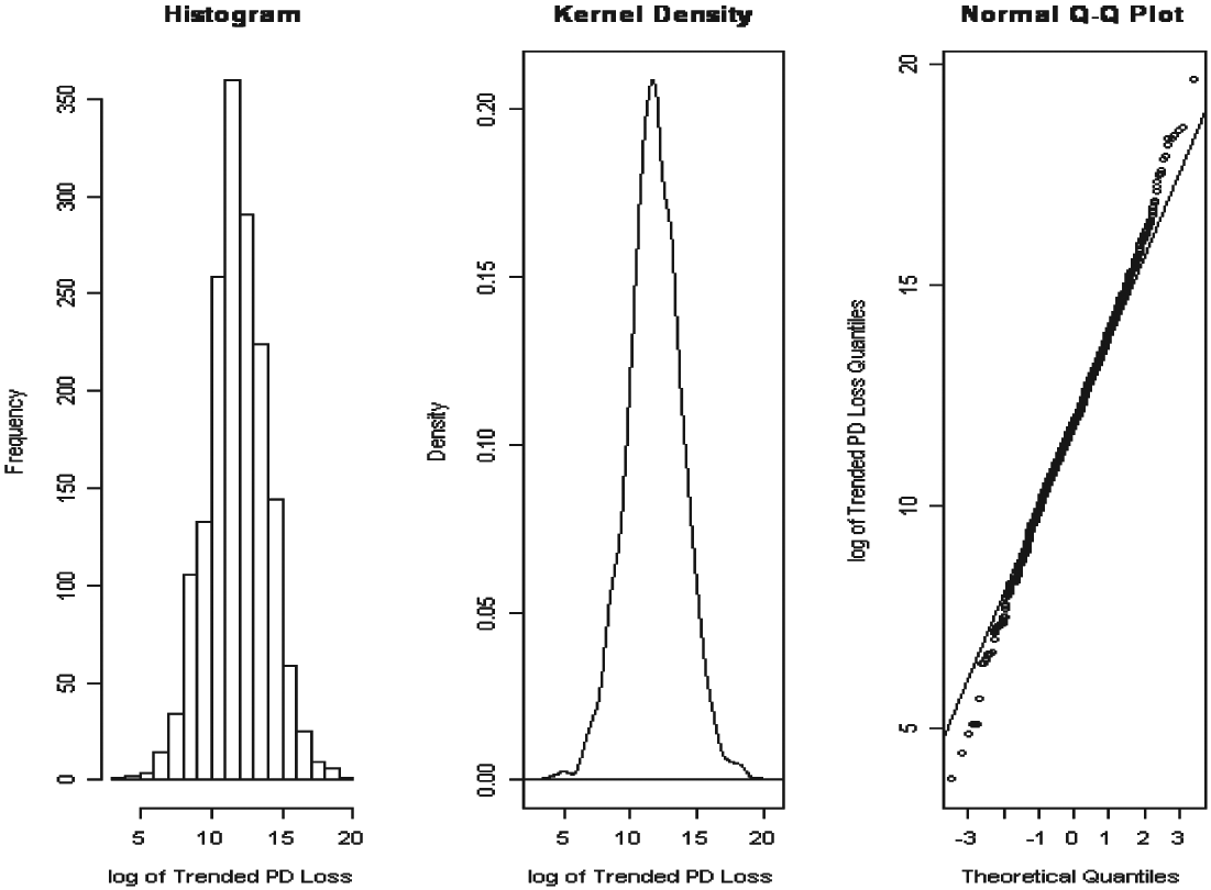
Clues to the shape of the underlying distribution for X₁ may be obtained by plotting a histogram and a kernel density of X₁. In addition, a QQ-Plot can be utilized to examine if the data supports informally whether X₁ is distributed according to a hypothesized probability distribution. Appendix 2 provides more information about these tools.

Figure 1 displays the histogram, kernel density, and QQ-Plot for X₁, based on the log of the trended PD losses contributing to the cell S(+,+). The left panel and the middle panel exhibit an approximately bell-shaped curve for the distribution of X₁. The kernel density provides a smoothed version of the histogram, as the shape of histograms tend to be affected by the specification of the number of bins and their spacing on the horizontal axis. The right panel of Figure 1, the QQ-Plot, compares the expected (according to normal) and actual quantiles. The majority of the points lie about a straight line. Hence, the plots in Figure 1 suggest that it is reasonable to assume that X₁ may be represented as normal.

Figure 2 is similar to Figure 1, but applies to X₂. It is based on the log of the trended TE losses contributing to the cell S(+,+). Once again the plots in Figure 2 suggest that it is reasonable to assume that X₂ may be normally distributed.

Figures 1 and 2 support informally the reasonableness of the assumption that X₁ and X₂ are normally distributed; hence it is natural to consider a bivariate normal, X, to represent (X₁,X₂).

The bivariate probability distributions considered in this paper are:

1. bivariate lognormal distribution Y,

2. bivariate normal distribution X, and

3. standardized bivariate normal Z.

These three distributions are related to each other according to

\[ \binom{Y_{1}}{Y_{2}}=\binom{\exp \left(X_{1}\right)}{\exp \left(X_{2}\right)}=\binom{\exp \left(\mu_{1}+\sigma_{1} Z_{1}\right)}{\exp \left(\mu_{2}+\sigma_{2} Z_{2}\right)} \]

where μ_i​s and σ_i​s are parameters of a bivariate normal X as defined below.

The distributions of Y and Z may be derived from X. Hence, the focus will be on the bivariate normal distribution X.

The bivariate normal distribution X has parameters (μ,∑) where

\[ \mu=\binom{\mu_{1}}{\mu_{2}} \]

is the mean vector, and

\[ \Sigma=\left(\begin{array}{cc} \sigma_{1}^{2} & \rho \sigma_{1} \sigma_{2} \\ \rho \sigma_{1} \sigma_{2} & \sigma_{2}^{2} \end{array}\right) \]

is the variance-covariance matrix. The interpretation of the five parameters of X—(μ₁, μ₂, σ₁, σ₂, and ρ)—in terms of the moments of the components of X are as follows:

\[ \begin{aligned} \mu_{1} & =E\left(X_{1}\right), \quad \mu_{2}=E\left(X_{2}\right), \\ \sigma_{1}^{2} & =\operatorname{Var}\left(X_{1}\right), \quad \sigma_{2}^{2}=\operatorname{Var}\left(X_{2}\right), \quad \text { and } \\ \rho & =\frac{\operatorname{Cov}\left(X_{1}, X_{2}\right)}{\sigma_{1} \sigma_{2}} \end{aligned} \]

where ρ denotes the correlation between X₁ and X₂.

The bivariate lognormal Y is derived from X by exponentiation of the X₁ and X₂ components of X. It has the same parameters (μ,∑) as X.

The standardized bivariate normal Z is derived from X by standardizing the components of X, i.e., by replacing X_i​s by Z_i = (X_i − μ_i)/σ_i, i = 1, 2. It has a single parameter ρ.

If the data supports the notion that it is reasonable to assume a bivariate normal distribution for X, then it follows that it is also reasonable to assume that Y has a bivariate lognormal distribution.

In order to examine if the data supports the assumption of the bivariate normality for X, it is necessary to compute certain statistics of interest from the data as described below. These statistics depend upon the estimate of the parameters (μ,∑), i.e., upon the maximum likelihood estimates (µ̂, ∑̂). The maximum likelihood estimates of the five parameters (µ̂₁,µ̂₂,ŝ₁,ŝ₂,ρ̂) of a bivariate normal X are

\[ \begin{aligned} \hat{\mu} & =\binom{\hat{\mu}_{1}}{\hat{\mu}_{2}}, \quad \hat{\mu}_{1}=\bar{x}_{1}=\frac{1}{n} \sum_{i=1}^{n} x_{1, i}, \\ \hat{\mu}_{2} & =\bar{x}_{2}=\frac{1}{n} \sum_{i=1}^{n} x_{2, i}, \\ \hat{\Sigma} & =\frac{(n-1)}{n} S, \quad S=\left(\begin{array}{ll} s_{11} & s_{12} \\ s_{21} & s_{22} \end{array}\right), \\ s_{11} & =\frac{1}{n-1} \sum_{i=1}^{n}\left(x_{1, i}-\bar{x}_{1}\right)^{2}, \\ s_{22} & =\frac{1}{n-1} \sum_{i=1}^{n}\left(x_{2, i}-\bar{x}_{2}\right)^{2}, \end{aligned} \]

\[ \begin{aligned} s_{12} & =s_{21}=\frac{1}{n-1} \sum_{i=1}^{n}\left(x_{1, i}-\bar{x}_{1}\right)\left(x_{2, i}-\bar{x}_{2}\right), \\ \hat{\sigma}_{1} & =\sqrt{\frac{(n-1)}{n}} s_{11}, \quad \hat{\sigma}_{2}=\sqrt{\frac{(n-1)}{n} s_{22}}, \\ \hat{\rho} & =\frac{s_{12}}{\sqrt{s_{11} s_{22}}}, \end{aligned} \]

where

\[ x_{1, i}=\log (i \text { th trended PD loss }), \quad 1 \leq i \leq n, \]

and

\[ x_{2, i}=\log (i \text { th trended TE loss }), \quad 1 \leq i \leq n . \]

The matrix S above is the unbiased estimator for the ∑, while ∑̂ is the maximum likelihood estimator for ∑, which is a biased estimator.

Based on the trended losses contributing to the cell S(+,+) only, the maximum likelihood estimate of the five parameters were

\[ \begin{array}{ll} \hat{\mu}_{1}=11.830, & \hat{\mu}_{2}=11.057, \\ \hat{\sigma}_{1}=2.086, & \hat{\sigma}_{2}=2.399, \text { and } \hat{\rho}=0.646 . \end{array} \]

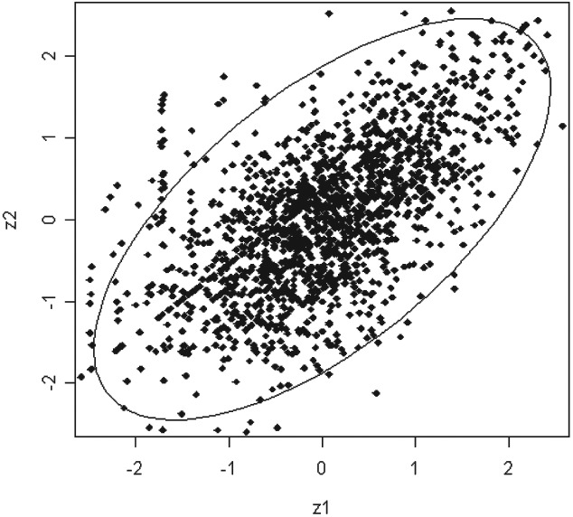
The informal support of the bivariate normality of X lies in the use of two graphs: Figure 3 (Ellipse) and Figure 4 (QQ-Plot), see below. The theory underlying the constructions of these two figures rests upon a result, referred here to as Theorem 1 (see below), from the subject of multivariate statistical analysis (see Johnson and Wichern 2002).

If the random vector X has a bivariate normal distribution with parameters (μ,∑), then the random variable Q, a quadratic form,

\[ Q=\left(X_{1}-\mu_{1}, X_{2}-\mu_{2}\right)^{\prime} \Sigma^{-1}\binom{X_{1}-\mu_{1}}{X_{2}-\mu_{2}} \tag{1} \]

is distributed as a chi-square distribution with 2 degrees of freedom.

Based on Theorem 1, provided that X is assumed to be distributed as a bivariate normal, then the following probability statement can be made: The chance that

\[ Q \leq \chi_{2}^{2}(0.95) \tag{2} \]

is 95%, where χ₂²(0.95) denotes the 95th quantile of a chi-square distribution with two degrees of freedom.

In order to create Figure 3 based on inequality (2), two changes must be made. First, the X₁ and X₂ random variables are replaced by the Z₁ and Z₂ variables, the standardized version of the X₁ and X₂. Second, the parameters (μ,∑) are replaced by their sample estimates (µ̂, ∑̂ ) in order to compute the values of Z₁ and Z₂ from the data. After making these two changes, then the inequality (2) becomes

\[ \hat{Q}=\frac{1}{1-\hat{\rho}^{2}}\left[Z_{1}^{2}-2 \hat{\rho} Z_{1} Z_{2}+Z_{2}^{2}\right] \leq \chi_{2}^{2}(0.95) . \tag{3} \]

The ellipse in Figure 3 is based on plotting the observed values of (z₁,z₂) subject to the inequality (3).

Table 4 provides additional figures for the 50% and 90% expected and actual coverage probabilities based on the assumption of the bivariate normality of X. There is a close agreement between expected and actual coverage probabilities in Table 4, especially for the higher probability levels. Thus, Figure 3 and Table 4 support informally that it is reasonable to state that X has a bivariate normal distribution.

If the premise of bivariate normality is not tenable, then a search should be made for another bivariate distribution, or alternatively, use copulas in conjunction with marginal distributions of Y₁ and Y₂ as deemed appropriate; see Nelson (2006) regarding copulas.

In this paper, a single bivariate lognormal distribution has been considered to represent the loss distribution. No distinction has been made with respect to the risk attributes. Thus, the same distribution is implied for risks with differing construction types, protection, or size. The size may be represented by the location value and/or the business interruption limit. If it is desirable to have a family of bivariate lognormal distributions, differing by risk characteristics, then one way to accomplish this goal may be by incorporating these risk attributes into the parameters (μ,∑). For example, to account for the effect of the size of the risk, one can replace the parameters (μ,∑) by parameters (μ*,Z) according to

\[ \mu^{*}=\binom{\mu_{1}^{*}}{\mu_{2}^{*}}=\binom{\beta_{0,1}+\beta_{1,1} \log (\text { PD Value })}{\beta_{0,2}+\beta_{1,2} \log (\text { TE Limit })} . \]

Here, the regression-like parameters β_0,1, β_1,1, β_0,2, and β_1,2 need to be estimated from the data. A nonlinear estimation procedure, similar to the GLM approach, may be used to estimate all the model parameters. However, this topic is not pursued further in this paper.

Another graphical procedure for illustrating informally the reasonableness of the assumption of the bivariate normality is the use of the QQ-Plot—Figure 4 below. In order to create this figure, it is necessary first to introduce the notion of “Squared Generalized Distance” statistics, d_j²s, (see Johnson and Wichern 2002):

\[ \begin{array}{c} d_{j}^{2}=\left(X_{1, j}-\hat{\mu}_{1}, X_{2, j}-\hat{\mu}_{2}\right)^{\prime} S^{-1}\binom{X_{1, j}-\hat{\mu}_{1}}{X_{2, j}-\hat{\mu}_{2}}, \\ j=1,2, \ldots, n . \end{array} \tag{4} \]

These statistics like the random variable Q, in Equation (1), are quadratic forms which can be computed from the data since the parameters (μ,∑) of the bivariate normal have been replaced by their sample estimates (µ̂,S), see above. Assuming that X has a bivariate normal distribution, Theorem 1 implies that the d² statistics constitute a sample of size n that is approximately distributed as a chi-square with two degrees of freedom. The approximate nature of this result is due to the fact that the parameters (μ,∑) have been replaced by their estimates. The QQ-Plot, Figure 4, was obtained by plotting the expected quantiles from a chi-square distribution with two degrees of freedom on the horizontal axis against the actual observed quantiles of d_j²s as plotted on the vertical axis. (Refer to Appendix 3 for more details.)

Figure 4 shows that the majority of points lie close to a straight line, suggesting the reasonableness of the assumption of the bivariate normality.

5. Specification of claim payment function

The potential insured loss amounts Y₁ (PD loss) and Y₂ (TE loss) are affected by loss-sensitive provisions of a policy. In this paper, the loss-sensitive provisions are comprised of a PD deductible D₁, a TE deductible D₂, an attachment point A, and a combined limit of L. The interaction of losses, Y′ = (Y₁,Y₂), with loss-sensitive provisions (D₁,D₂,A,L) is defined through the CPF, denoted by g(Y₁,Y₂), see below.

Before discussing the specification of a CPF in a multivariate setting, it may be instructive to review the form of the CPF in a univariate situation. For a single cover policy with a deductible D, and limit L, let the random variable X denote an insured loss. Then the CPF, designated by h(X) is

\[ \begin{aligned} h(X) & =\min \{\max (X-D, 0), L\} \\ & =\min (X, D+L)-\min (X, D) . \end{aligned} \tag{5} \]

The expected value of the h(X), E[h(X)], denotes the severity component of pure premium—the ALC, and can be stated as

\[ E[h(X)]=\operatorname{LEV}(D+L)-\operatorname{LEV}(D) \tag{6} \]

where LEV(c) is the limited expected value of the loss amount X subject to a cap c. It is computed as

\[ \operatorname{LEV}(c)=\int_{0}^{\infty} \min (x, c) d F(x) \]

where F denotes the cdf of the insured loss X.

In the case of X being distributed as a lognormal with parameters (μ,σ²), then the LEV(c) function is

\[ \begin{aligned} \operatorname{LEV}(c)= & e^{\mu+1 / 2 \sigma^{2}} \Phi\left(\frac{\log (c)-\mu-\sigma^{2}}{\sigma}\right) \\ & +c\left[1-\Phi\left(\frac{\log (c)-\mu}{\sigma}\right)\right] \end{aligned} \tag{7} \]

where Φ is the cdf of a standard normal.

Thus, in the lognormal case, it is easy to compute the expected value of the CPF using (6) and (7). Simply use the exponential function and the cdf of the standard normal, Φ. However, the computation of the ALC for multiple cover policies is more complicated, as explained below.

For a multiple cover policy with a potential PD loss amount y₁ and a TE loss amount y₂, subject to loss-sensitive features, (D₁,D₂,A,L), the CPF as denoted by g(y₁,y₂) cannot be expressed by a single formula and has to be defined piecemeal. What is needed is a breakup of the positive quadrant, R₊² = [0,∞) × [0,∞), into ten regions, as defined below. Then, the value of g(y₁,y₂) can be determined depending upon the region where the point (y₁,y₂) will reside.

The ten required regions are defined as

1. R₁ = {(y₁,y₂): y₁ ≤ D₁, y₂ ≤ D₂}

2. R₂ = {(y₁,y₂): y₁ ≤ D₁, D₂ < y₂ ≤ D₂ + A}

3. R₃ = {(y₁,y₂): y₁ ≤ D₁, D₂ + A < y₂ ≤ D₂ + A + L}

4. R₄ = {(y₁,y₂): y₁ ≤ D₁, y₂ > D₂ + A + L}

5. R₅ = {(y₁,y₂): D₁ < y₁ ≤ D₁ + A, y₂ ≤ D₂}

6. R₆ = {(y₁,y₂): D₁ + A < y₁ ≤ D₁ + A + L, y₂ ≤ D₂}

7. R₇ = {(y₁,y₂): y₁ > D₁ + A + L, y₂ ≤ D₂}

8. R₈ = {(y₁,y₂): y₁ > D₁, y₂ > D₂, y₁ + y₂ ≤ D₁ + D₂ + A}

9. R₉ = {(y₁,y₂): y₁ > D₁, y₂ > D₂, D₁ + D₂ + A < y₁ + y₂ ≤ D₁ + D₂ + A + L}

10. R₁₀ = {(y₁,y₂): y₁ > D₁, y₂ > D₂, y₁ + y₂ > D₁ + D₂ + A + L}.

The diagram (Figure 5) depicts these regions. These regions are used to integrate the function g(y₁,y₂) over the positive quadrant, as explained in Appendix 4. For illustrative purposes, the values chosen for these loss-sensitive features are D₁ = 1, D₂ = 1, A = 4, and L = 4.

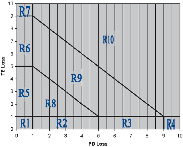
The following will illustrate how g(y₁,y₂) is computed according to the region. For region 1, R₁ = {(y₁,y₂): y₁ ≤ D₁, y₂ ≤ D₂}, the value of g(y₁,y₂) is zero, since both losses are below their respective deductibles. For region 2, R₂ = {(y₁,y₂): y₁ ≤ D₁, D₂ < y₂ ≤ D₂ + A}, the value of g(y₁,y₂) is also zero. In this case y₁, the PD loss, is below its deductible D₁. The TE loss, y₂, exceeds its deductible D₂, but due to the imposition of the attachment A, the constraint: y₂ − D₂ ≤ A, there is no loss payment to be made. For region 3, R = {(y₁,y₂): y₁ ≤ D₁, D₂ + A < y₂ ≤ D₂ + A + L}, the CPF is given by g(y₁,y₂) = min{max(y₂ − (D₂ + A), 0), L}. Similar expressions for g(y₁,y₂) may be written in terms of y₁, y₂, D₁, D₂, A and L depending on the region applied. In a computing environment, expressions for the g(y₁,y₂) may be written in terms of if-then-else based on the region.

6. Computation of average loss cost based on bivariate lognormal

In this section, an algorithm is outlined for computing the ALC, the severity component of the pure premium. The following formula, (8), may be used as the basis of calculating the pure premium. This formula takes into consideration the way the data was organized in Section 3 by Table 1 and Table 2.

\[ \begin{aligned} \text { Pure Premium }= & \text { Freq }_{\mathrm{PD}} \text { ALC }_{\mathrm{PD}}+\text { Freq }_{\mathrm{TE}} \text { ALC }_{\mathrm{TE}} \\ & + \text { Freq }_{\mathrm{PD} \& \mathrm{TE}} \text { ALC }_{\mathrm{PD} \& \mathrm{TE}} \end{aligned} \tag{8} \]

where Freq_PD, Freq_TE, and Freq_PD&TE are frequency values, and ALC_PD, ALC_TE, and ALC_PD&TE are ALC values.

The ALC_PD and ALC_TE can be computed using appropriate univariate SOLD based on trended loss data fitted to cells S(+,NA) and S(NA,+), respectively. In this paper, the interest lies only in explaining how to estimate ALC_PD&TE based on a bivariate lognormal distribution.

In Section 4, the data was fitted to losses arising from cell S(+,+). A bivariate lognormal distribution was considered to represent the SOLD, and its five parameters were estimated from the data. In Section 5, the form of the CPF, the function g(y₁,y₂), was described in terms of the interaction of loss data (y₁,y₂) with loss-sensitive features, (D₁,D₂,A,L). Finally, an expression for ALC can be provided by defining the ALC as a double integral

\[ \begin{array}{l} \operatorname{ALC}_{\text {PD&TE }}\left(D_{1}, D_{2}, A, L ; \mu, \Sigma\right) \\ \quad=\iint g\left(y_{1}, y_{2}\right) f_{Y_{1}, Y_{2}}\left(y_{1}, y_{2}\right) d y_{1} d y_{2} \end{array} \tag{9} \]

where (D₁,D₂,A,L) is loss-sensitive provisions of the multiple cover policy,

(μ,∑) are the parameters of the bivariate lognormal distribution replaced by their sample estimates,

g(y₁,y₂) is the CPF as described in Section 5, and

\(f_{y_1, y_2}(y_1, y_2)\) is the density function of a bivariate lognormal (see Section 4 and Appendix 3).

What is required is an estimate for the above double integral. Since the computation of (9) is rather technical, it has been supplied in Appendices 4 and 5.

Table 5 provides estimates of ALC_PD&TE(D₁,D₂,A,L;μ,∑) by considering differing loss-sensitive provisions. Such a table is useful in assessing the impact of (D₁,D₂,A,L) upon ALC_PD&TE(D₁,D₂,A,L;μ,∑).

It should be noted that the figures in Table 5 are based on the value of the estimated parameters, as well as selection of the value of N (N = 100). The variable N implicitly controls the error incurred in estimating ALC (see Appendix 4 for the definition and use of the N term). The computation time to estimate ALC in Table 4 was a matter of a few seconds for the case of N = 100. For the case of N = 1000 it was less than two minutes.

The algorithm outlined above estimates ALC, a double integral, using a numerical procedure that approximates the double integral (9) by a suitable sum as explained in Appendix 4. An alternative numerical procedure to estimate ALC can be based on simulation. The simulation approach requires generating random pairs (y₁,y₂) according to a bivariate lognormal whose parameters (μ,∑) have been estimated from the data (see Section 4). Then, for each simulated pair (y₁,y₂), the value of CPF, g(y₁,y₂), is calculated based upon the ten regions in which (y₁,y₂) resides (see Section 5). This procedure is repeated a number of times and the corresponding generated g(y₁,y₂) values are averaged to provide an alternative estimate for the ALC. An important step in the simulation procedure is generating samples from a bivariate lognormal distribution. Appendix 6 provides an algorithm for doing this and discusses briefly some advantages as well as drawbacks of the simulation approach.

7. Conclusions

This paper discussed pricing a property policy with multiple cover for PD and TE subject to an attachment point, separate deductibles, and a combined limit relying on a bivariate lognormal distribution. Comparisons were made between univariate and multivariate curve fitting. A methodology needed to fit a bivariate lognormal to the data was developed. An algorithm was given for estimating the ALC, a double integral. Hopefully, this paper will encourage other actuaries to contribute further to the methodology needed for pricing multiple cover policies and the applications of multivariate statistical techniques to the actuarial field.

---

Acknowledgement

The author has benefited from discussions of this subject with Shane Vadbunker, and in particular would like to thank him for writing an Excel VBA program to estimate average loss cost based on the bivariate lognormal distribution.