Prediction Error of the Multivariate Additive Loss Reserving Method for Dependent Lines of Business

undefined

1. Introduction and motivation

1.1. Claims reserving

Often in non-life insurance, claims reserves are the largest position on the liability side of the balance sheet. Therefore, given the available information about the past, the prediction of an adequate amount of claim liability assumed by the non-life insurance company, as well as the quantification of the uncertainties in these reserves, is a major task in actuarial practice and science [e.g., Taylor (2000); Wüthrich and Merz (2008); Casualty Actuarial Society (2001); Teugels and Sundt (2004); England and Verrall (2002)].

1.2. Multivariate claims reserving methods and their conditional MSEP

In the present paper, we consider the claims reserving problem for a portfolio consisting of several correlated run-off subportfolios. This simultaneous study of several individual run-off subportfolios is motivated by the following considerations:

• In practice it is quite natural to subdivide a non-life run-off portfolio into several correlated subportfolios, such that each subportfolio satisfies certain homogeneity properties (e.g., the chain-ladder assumptions or the assumptions of the additive method).

• It addresses the problem of dependence between the run-off portfolios of different lines of business (e.g., between auto liability and general liability business).

• The multivariate approach has the advantage that by observing one run-off subportfolio we can learn about the behavior of the other runoff subportfolios (e.g., subportfolios of small and large claims).

• It resolves the problem of additivity (i.e., the estimators of the ultimate claims for the whole portfolio are obtained by summation over the estimators of the ultimate claims for the individual run-off subportfolios).

However, in the case of correlated run-off subportfolios, the calculation of the conditional mean square error of prediction (MSEP) for the predictor of the ultimate claim size of the total portfolio is more sophisticated than the calculation of the conditional MSEP for the predictor of the ultimate claim size of a single run-off subportfolio.

An alternative idea to the simultaneous study of several individual run-off subportfolios is to calculate the reserves and their uncertainties only for the total aggregated run-off portfolio. However, one should pay attention to the fact that if the subportfolios satisfy, for example, the assumptions of the chain-ladder or the assumptions of the additive method, the aggregated run-off portfolio does not in general satisfy these assumptions (Ajne 1994; Klemmt 2004). Therefore, in most cases it is not a promising solution to study the aggregated portfolio for the claims reserving problem of several run-off subportfolios.

Holmberg (1994) was probably the first one to investigate the problem of dependence between run-off portfolios of different lines of business. Later Halliwell (1997) and Quarg and Mack (2004) [see also Merz and Wüthrich (2006)] proposed the first bivariate models which express the dependence between the paid and incurred losses of a single run-off subportfolio.

Braun (2004) generalized the well-known univariate chain-ladder model of Mack (1993) to the bivariate case by incorporating correlations between two run-off subportfolios. In this setup he derived an estimate for the conditional MSEP for the predictor of the ultimate claim size of two correlated run-off subportfolios. Using a multivariate time-series model for the chain-ladder method Merz and Wüthrich (2007) gave an estimator for the conditional MSEP in the case of N correlated run-off subportfolios. However, both the Braun (2004) approach and the Merz and Wüthrich (2007) approach have the disadvantage that the chain-ladder factors are estimated in a univariate way. This means the estimation of the chain-ladder factors is restricted to the data of the respective individual run-off subportfolio and therefore does not take into account the correlation structure between the different runoff subportfolios. Pröhl and Schmidt (2005) and Schmidt (2006b) showed that these univariate estimates of the chain-ladder factors are not optimal in terms of a classical optimality criterion in the case of correlated run-off subportfolios and therefore one should replace the univariate estimators with multivariate estimators of the chainladder factors reflecting the correlation structure. However, their study did not go beyond best estimators; that is, they did not derive an estimator for the conditional MSEP for the predictor of the ultimate claim size of the total portfolio. Finally, using a multivariate chain-ladder timeseries model, Merz and Wüthrich (2008) derived an estimate for the conditional MSEP, in which the chain-ladder factors are estimated in a multivariate way. That is, Merz and Wüthrich (2008) studied the conditional MSEP for the multivariate chain-ladder estimates proposed by Pröhl and Schmidt (2005) and Schmidt (2006b).

1.3. Multivariate additive loss reserving method

The multivariate additive loss reserving method proposed by Hess, Schmidt, and Zocher (2006) and Schmidt (2006b) is based on a multivariate linear model which is suitable for certain portfolios consisting of several correlated run-off subportfolios. The additive loss reserving method has the following features:

1. It is a very simple claims reserving method which can easily be implemented in a spreadsheet.

2. Unlike the chain-ladder method, the additive loss reserving method combines past observations in the upper claims development triangle with external knowledge from experts or with a priori information (e.g., premium, number of contracts, data from similar run-off portfolios, and market statistics).

3. It is applied to incremental data and thus allows for modeling negative incremental claims in contrast to some other models such as the (overdispersed) Poisson model [cf. Wüthrich and Merz (2008)]. This makes the additive loss reserving method suitable for the use of incurred data, which often exhibits negative incremental values in later development years due to earlier overestimation of case reserves.

4. Unlike the chain-ladder method, the prediction for the ultimate claim does not depend completely on the last observation on the diagonal. This means an outlier on the diagonal will not be projected directly to the ultimate claim. Therefore, the additive loss reserving method is more robust to outliers in the last observations than the chain-ladder method.

Under the assumptions of their multivariate additive loss reserving model, Hess, Schmidt, and Zocher (2006) and Schmidt (2006b) derived a formula for the Gauss-Markov predictor for the nonobservable incremental claim sizes which is optimal in terms of a classical optimality criterion. The components of these predictors are different from the predictors of the univariate additive loss reserving method if the subportfolios are correlated (e.g., see Schmidt (2006b, 2006a) for the univariate additive loss reserving method). This means that the predictors of the univariate method are not optimal in the case of correlated subportfolios. However, Hess, Schmidt, and Zocher (2006) and Schmidt (2006b) did not derive an estimator of the conditional MSEP for the multivariate additive loss reserving method. Since in actuarial practice and science the conditional MSEP is a very popular measure to quantify the uncertainties in claims reserves, this paper aims to fill that gap. These studies of uncertainty are especially crucial in the development of new solvency guidelines where one exactly quantifies the risk profile of the different insurance companies.

More precisely, we formulate a stochastic model for the multivariate additive loss reserving method to derive an estimator for the conditional MSEP using the Gauss-Markov predictor proposed by Hess, Schmidt, and Zocher (2006) and Schmidt (2006b). Furthermore, by means of a detailed example, this estimator is then compared to the estimator for the conditional MSEP of the univariate predictor (i.e., if we ignore the correlation structure between individual subportfolios) as well as to the estimator for the conditional MSEP of the multivariate chain-ladder methods considered by Braun (2004) and Merz and Wüthrich (2008).

2. Notation and multivariate framework

In the sequel we assume that the data for the N ≥ 1 run-off subportfolios consist of run-off triangles of observations of the same size. However, the multivariate additive loss reserving method can also be applied to other shapes of data (e.g., run-off trapezoids). In these N triangles the indices

1. n, 1 ≤ n ≤ N, refer to subportfolios (triangles),

2. i, 0 ≤ i ≤ I, refer to accident years (rows), and

3. j, 0 ≤ j ≤ J, refer to development years (columns).

Figure 1 shows the claims data structure for the N claims development triangles described above.

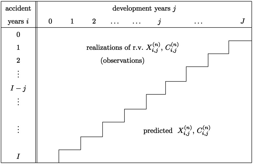
The incremental claims (i.e., incremental payments, change of reported claim amount, or number of reported claims with reporting delay $j$ ) of run-off triangle $n$ for accident year $i$ and development year $j$ are denoted by $X_{i, j}^{(n)}$ and cumulative claims (i.e., cumulative payments, claims incurred, or total number of reported claims) of accident year $i$ up to development year $j$ are given by

$$C_{i, j}^{(n)}=\sum_{k=0}^{j} X_{i, k}^{(n)} . \tag{1}$$

We assume that the last development year is given by $J$, that is $X_{i, j}^{(n)}=0$ for all $j>J$, and the last accident year is given by $I$. Moreover, our assumption that we consider run-off triangles implies $I=J$.

Usually, at time I, we have observations

$$\mathcal{D}_{I}^{(n)}=\left\{X_{i, j}^{(n)} ; i+j \leq I\right\}, \tag{2}$$

for all run-off subportfolios n ∈ {1, . . . , N}. This means that at time I (calendar year I) we have a total of observations over all subportfolios

$$\mathcal{D}_{I}^{N}=\bigcup_{n=1}^{N} \mathcal{D}_{I}^{(n)}, \tag{3}$$

and we need to predict the random variables in its complement

$$\mathcal{D}_{I}^{N, c}=\left\{X_{i, j}^{(n)} ; i \leq I, i+j>I, 1 \leq n \leq N\right\} . \tag{4}$$

For the derivation of the conditional MSEP for several run-off subportfolios, it is convenient to write the data of the N subportfolios in vector form. Thus, we define the N-dimensional random vectors of incremental and cumulative payments by

$$\begin{array}{l} \mathbf{X}_{i, j}=\left(X_{i, j}^{(1)}, \ldots, X_{i, j}^{(N)}\right)^{\prime} \quad \text { and }\\ \mathbf{C}_{i, j}=\left(C_{i, j}^{(1)}, \ldots, C_{i, j}^{(N)}\right)^{\prime} \end{array} \tag{5}$$

for i ∈ {0, . . . , I} and j ∈ {1, . . . , J}. Moreover, we define the N-dimensional column vector consisting of ones by

$$\mathbf{1}=(1, \ldots, 1)^{\prime} \in \mathbb{R}^{N} \tag{6}$$

and denote by

$$\mathrm{D}(\mathbf{a})=\left(\begin{array}{lll} a_{1} & & 0 \\ & \ddots & \\ 0 & & a_{N} \end{array}\right) \tag{7}$$

the $N \times N$-diagonal matrix of the vector $\mathbf{a}= \left(a_1, \ldots, a_N\right)^{\prime} \in \mathbb{R}^N$.

3. Multivariate additive loss reserving method

The additive loss reserving method is easy to apply. It is based on the study of individual incremental loss ratios. We define for i ∈ {0, . . . , I} and j ∈ {1, . . . , J} the N-dimensional vector of individual incremental loss ratios for accident year i and development year j by

$$\mathbf{M}_{i, j}=\left(M_{i, j}^{(1)}, \ldots, M_{i, j}^{(N)}\right)^{\prime}=\mathrm{V}_{i}^{-1} \cdot \mathbf{X}_{i, j}, \tag{8}$$

with a volume measure

$$\mathrm{V}_{i}=\left(\begin{array}{ccccc} V_{i}^{(1,1)} & V_{i}^{(1,2)} & \ldots & \ldots & V_{i}^{(1, N)} \\ V_{i}^{(2,1)} & V_{i}^{(2,2)} & \ldots & \ldots & V_{i}^{(2, N)} \\ \vdots & \vdots & \ddots & & \vdots \\ \vdots & \vdots & & \ddots & \vdots \\ V_{i}^{(N, 1)} & V_{i}^{(N, 2)} & \ldots & \ldots & V_{i}^{(N, N)} \end{array}\right), \tag{9}$$

which is a deterministic positive definite symmetric $N \times N$-matrix. The component $M_{i, j}^{(n)}$ of $\mathbf{M}_{i, j}$ denotes the individual incremental loss ratio (relative to $V_i$ ) for accident year $i$ and development year $j$ of subportfolio $n$.

In the univariate case N = 1 we have

$$M_{i, j}=X_{i, j} / V_{i}, \tag{10}$$

where V_i is an appropriate (deterministic) volume measure. If X_i,j denotes incremental payments and V_i is the total premium received for accident year i, then M_i,j tells how the total loss ratio is paid over time.

3.1. Multivariate additive loss reserving model

The following multivariate additive loss reserving model is a special case of the multivariate claims reserving model studied by Hess, Schmidt, and Zocher (2006) and Schmidt (2006b).

• Incremental payments of different accident years i are independent.

• There exist $N \times N$-dimensional deterministic positive definite symmetric matrices $\mathrm{V}_0, \ldots, \mathrm{~V}_I$ and $N$-dimensional constants $(j=1, \ldots, J)$ $$\begin{aligned}\mathbf{m}_{j} & =\left(m_{j}^{(1)}, \ldots, m_{j}^{(N)}\right)^{\prime} \quad \text { and } \\\sigma_{j-1} & =\left(\sigma_{j-1}^{(1)}, \ldots, \sigma_{j-1}^{(N)}\right)^{\prime}\end{aligned} \tag{11}$$ with $\sigma_{j-1}^{(n)}>0$ for all $n=1, \ldots, N$ as well as $N$ dimensional random variables $$\varepsilon_{i, j}=\left(\varepsilon_{i, j}^{(1)}, \ldots, \varepsilon_{i, j}^{(N)}\right)^{\prime}, \tag{12}$$ such that for all i ∈ {0, . . . , I} and j ∈ {1, . . . , J} we have $$\mathbf{X}_{i, j}=\mathrm{V}_{i} \cdot \mathbf{m}_{j}+\mathrm{V}_{i}^{1 / 2} \cdot \mathrm{D}\left(\varepsilon_{i, j}\right) \cdot \boldsymbol{\sigma}_{j-1} . \tag{13}$$ Moreover, the random variables $\varepsilon_{i, j}$ are independent with $E\left[\varepsilon_{i, j}\right]=\mathbf{0}$ and

  $$\begin{array}{l} \operatorname{Cov}\left(\varepsilon_{i, j}, \varepsilon_{i, j}\right) \\ \quad=E\left[\varepsilon_{i, j} \cdot \varepsilon_{i, j}^{\prime}\right]=\left(\begin{array}{ccccc} 1 & \rho_{j-1}^{(1,2)} & \cdots & \cdots & \rho_{j-1}^{(1, N)} \\ \rho_{j-1}^{(2,1)} & 1 & \cdots & \cdots & \rho_{j-1}^{(2, N)} \\ \vdots & \vdots & \ddots & & \vdots \\ \vdots & \vdots & & \ddots & \vdots \\ \rho_{j-1}^{(N, 1)} & \rho_{j-1}^{(N, 2)} & \cdots & \cdots & 1 \end{array}\right), \end{array} \tag{14}$$ where $\rho_{j-1}^{(n, m)} \in(-1,1)$ for $n, m \in\{1, \ldots, N\}$ and $n \neq m$.

Clearly, in most practical applications $V_i$ is chosen to be diagonal so as to represent a volume measure of accident year i, known a priori (e.g., premium, number of contracts, expected number of claims, etc.), or an estimate from external knowledge such as experts, similar portfolios, or market statistics (see Example in Section 6). However, we can also take into account that the volume measure or estimate from external knowledge for subportfolio $m$ influences the incremental payments for another subportfolio $n$ in accident year $i$ by choosing $V_i^{(n, m)} \neq 0$. In this case we obtain a nondiagonal matrix $V_i$.

In the univariate case N = 1, the additive model satisfies

$$X_{i, j} / V_{i}=m_{j}+V_{i}^{-1 / 2} \cdot \sigma_{j-1} \cdot \varepsilon_{i, j} ,\tag{15}$$

with

$$\begin{aligned} E\left[X_{i, j}\right] & =V_{i} \cdot m_{j} \quad \text { and } \\ \operatorname{Var}\left(X_{i, j}\right) & =V_{i} \cdot \sigma_{j-1}^{2} . \end{aligned} \tag{16}$$

Hence this model can also be interpreted as a GLM model with Gaussian variance function (i.e., $V(x)=1$ ), volume measure $V_i$ and dispersion parameter $\sigma_{j-1}^2$ [cf. McCullagh and Nelder (1989)].

Under Model Assumptions 3.1 we have

$$\operatorname{Cov}\left(\mathbf{X}_{i, j}, \mathbf{X}_{i, j}\right)=\mathrm{V}_{i}^{1 / 2} \cdot \Sigma_{j-1} \cdot \mathrm{~V}_{i}^{1 / 2}, \tag{17}$$

where

$$\begin{aligned} \Sigma_{j-1} & =\mathrm{E}\left[\mathrm{D}\left(\varepsilon_{i, j}\right) \cdot \boldsymbol{\sigma}_{j-1} \cdot \boldsymbol{\sigma}_{j-1}^{\prime} \cdot \mathrm{D}\left(\varepsilon_{i, j}\right)\right] \\ & =\mathrm{D}\left(\boldsymbol{\sigma}_{j-1}\right) \cdot \operatorname{Cov}\left(\varepsilon_{i, j}, \varepsilon_{i, j}\right) \cdot \mathrm{D}\left(\boldsymbol{\sigma}_{j-1}\right) \\ & =\left(\begin{array}{ccccc} \left(\sigma_{j-1}^{(1)}\right)^{2} & \sigma_{j-1}^{(1)} \sigma_{j-1}^{(2)} \rho_{j-1}^{(1,2)} & \cdots & \cdots & \sigma_{j-1}^{(1)} \sigma_{j-1}^{(N)} \rho_{j-1}^{(1, N)} \\ \sigma_{j-1}^{(2)} \sigma_{j-1}^{(1)} \rho_{j-1}^{(2,1)} & \left(\sigma_{j-1}^{(2)}\right)^{2} & \cdots & \cdots & \sigma_{j-1}^{(2)} \sigma_{j-1}^{(N)} \rho_{j-1}^{(2, N)} \\ \vdots & \vdots & & & \vdots \\ \vdots & \vdots & & & \vdots \\ \sigma_{j-1}^{(N)} \sigma_{j-1}^{(1)} \rho_{j-1}^{(N, 1)} & \sigma_{j-1}^{(N)} \sigma_{j-1}^{(2)} \rho_{j-1}^{(N, 2)} & \cdots & \cdots & \left(\sigma_{j-1}^{(N)}\right)^{2} \end{array}\right) . \end{aligned} \tag{18}$$

By Model Assumptions 3.1 we restrict any assumption regarding the correlation between the $N$ run-off subportfolios to each of the corresponding development years $j(j=1, \ldots, J)$ in the $N$ run-off triangles. Matrix $\Sigma_{j-1}$ reflects the correlation structure between the incremental claims of development year $j$ in the $N$ different subportfolios. Often correlations between different run-off subportfolios are attributed to claims inflation. Under this point of view, it may seem more reasonable to allow for correlation between the incremental claims of the same calender year (diagonals of the claims development triangles). However, this would contradict the assumption of independent accident years which is common to most claims reserving methods, and in fact also necessary to develop reasonable estimators from a mathematical point of view.

The Multivariate Additive Model 3.1 is a special case of the multivariate claims reserving model proposed by Hess, Schmidt, and Zocher (2006) and Schmidt (2006b), in contrast to which we assume that incremental payments $\mathbf{X}_{i, j}$ are independent (instead of only uncorrelated) and generated by the time series (13).

Remark 3.2

• The incremental claims $\mathbf{X}_{i, j}$ and $\mathbf{X}_{k, l}$ are independent for $i \neq k$ or $j \neq l$.
• The $N$-dimensional expected incremental loss ratios $\left(\mathbf{m}_j\right)_{1 \leq j \leq J}$ can be interpreted as a multivariate scaled expected reporting/cashflow pattern over the different development years.
• In (17) we use the notation $\Sigma_{j-1}$ instead of $\Sigma_j$ since it simplifies the comparability with the derivations and results in Merz and Wüthrich (2008).
• Since we assume that $\mathrm{V}_i$ is a positive definite symmetric matrix, there is a well-defined positive definite symmetric matrix $\mathrm{V}_i^{1 / 2}$ (called square root of $\mathrm{V}_i$ ) satisfying $\mathrm{V}_i=\mathrm{V}_i^{1 / 2} \cdot \mathrm{~V}_i^{1 / 2}$.

We obtain for the conditional expectation (best estimate) $E\left[\mathbf{C}_{i, J} \mid \mathcal{D}_I^N\right]$ of the ultimate claim $\mathbf{C}_{i, J}$ :

Property 3.3. Under Model Assumptions 3.1 we have for all I−J + 1 ≤ i ≤ I

$$\begin{aligned} E\left[\mathbf{C}_{i, J} \mid \mathcal{D}_{I}^{N}\right] & =E\left[\mathbf{C}_{i, J} \mid \mathbf{C}_{i, I-i}\right] \\ & =\mathbf{C}_{i, I-i}+\mathrm{V}_{i} \cdot \sum_{j=I-i+1}^{J} \mathbf{m}_{j} . \end{aligned} \tag{19}$$

Proof Using the independence of the incremental claims we obtain

$$\begin{aligned} E\left[\mathbf{C}_{i, J} \mid \mathcal{D}_{I}^{N}\right] & =\mathbf{C}_{i, I-i}+E\left[\sum_{j=I-i+1}^{J} \mathbf{X}_{i, j} \mid \mathcal{D}_{I}^{N}\right] \\ & =\mathbf{C}_{i, I-i}+\sum_{j=I-i+1}^{J} E\left[\mathbf{X}_{i, j}\right] \\ & =\mathbf{C}_{i, I-i}+\mathrm{V}_{i} \cdot \sum_{j=I-i+1}^{J} \mathbf{m}_{j} \\ & =E\left[\mathbf{C}_{i, J} \mid \mathbf{C}_{i, I-i}\right]. \end{aligned} \tag{20}$$

This finishes the proof. Q.E.D.

This result motivates an algorithm for estimating the expected ultimate claims given the observation $\mathcal{D}_I^N$. If the $N$-dimensional expected incremental loss ratios $\left(\mathbf{m}_j\right)_{1 \leq j \leq J}$ are known, the expected outstanding claims liabilities of accident year $i$ for the $N$ correlated run-off triangles based on the information $\mathcal{D}_I^N$ are estimated by

$$E\left[\mathbf{C}_{i, J} \mid \mathcal{D}_{I}^{N}\right]-\mathbf{C}_{i, I-i}=\mathrm{V}_{i} \cdot \sum_{j=I-i+1}^{J} \mathbf{m}_{j}. \tag{21}$$

However, in most practical applications we have to estimate the ratios $\mathbf{m}_j$ from the data in the upper left triangle. Hess, Schmidt, and Zocher (2006) and Schmidt (2006b) propose the following multivariate estimates, for $j=1, \ldots, J$

$$\begin{aligned} \hat{\mathbf{m}}_{j}= & \left(\hat{m}_{j}^{(1)}, \ldots, \hat{m}_{j}^{(N)}\right)^{\prime} \\ = & \left(\sum_{i=0}^{I-j} \mathrm{~V}_{i}^{1 / 2} \cdot \Sigma_{j-1}^{-1} \cdot \mathrm{~V}_{i}^{1 / 2}\right)^{-1} \\ & \cdot \sum_{i=0}^{I-j}\left(\mathrm{~V}_{i}^{1 / 2} \cdot \Sigma_{j-1}^{-1} \cdot \mathrm{~V}_{i}^{1 / 2}\right) \cdot \mathbf{M}_{i, j} . \end{aligned} \tag{22}$$

The variable $\hat{m}_j^{(n)}$ denotes the estimated incremental loss ratio for development year $j$ and runoff triangle $n \in\{1, \ldots, N\}$ based on the information $\mathcal{D}_I^N$. Note that the covariance structure between the incremental claims in the different runoff subportfolios is incorporated into the estimation of $\mathbf{m}_j$ through the matrix $\Sigma_{j-1}$.

Hess, Schmidt, and Zocher (2006) and Schmidt (2006b) showed the following property, which states that the multivariate incremental loss ratio estimates (22) are optimal estimators of $\mathbf{m}_j$ with respect to the criterion of minimal expected squared loss.

Property 3.4. Under Model Assumptions 3.1, the estimator $\hat{\mathbf{m}}_j$ is an unbiased estimator for $\mathbf{m}_j$, which minimizes the expected squared loss among all $N$-dimensional linear combinations of the unbiased estimators $\left(\mathbf{M}_{l, j}\right)_{0 \leq l \leq I-j}$ for $\mathbf{m}_j$, i.e.,

$$\begin{array}{l} \mathrm{E}\left[\left(\mathbf{m}_{j}-\hat{\mathbf{m}}_{j}\right)^{\prime} \cdot\left(\mathbf{m}_{j}-\hat{\mathbf{m}}_{j}\right)\right] \\ =\min _{\mathrm{W}_{l, j} \in \mathbb{R}^{N \times N}} E\left[\left(\mathbf{m}_{j}-\sum_{l=0}^{I-j} \mathrm{~W}_{l, j} \cdot \mathbf{M}_{l, j}\right)^{\prime}\right. \\ \left.\cdot\left(\mathbf{m}_{j}-\sum_{l=0}^{I-j} \mathrm{~W}_{l, j} \cdot \mathbf{M}_{l, j}\right)\right] . \end{array} \tag{23}$$

Proof See proof of Theorem 4.1 in Schmidt (2006b). Q.E.D.

Note, in Property 3.4 we assume that the covariance matrix $\Sigma_{j-1}$ is known. However, if we do not have a reliable estimate for this covariance matrix it is often more appropriate in practice to use the univariate estimators. Property 3.4 motivates the following estimator for the conditionally expected ultimate claim:

Estimator 3.5 (Multivariate additive estimator) The multivariate additive estimator for $E\left[\mathbf{C}_{i, j} \mid \mathcal{D}_I^N\right]$ is for $i+j \geq I$ given by

$$\begin{aligned} {\widehat{\mathbf{C}_{i, j}}}^{\mathrm{AD}} & =\left({\widehat{C_{i, j}^{(1)}}}^{\mathrm{AD}}, \ldots,{\widehat{C_{i, j}^{(N)}}}^{\mathrm{AD}}\right)^{\prime} \\ & =\hat{E}\left[\mathbf{C}_{i, j} \mid \mathcal{D}_{I}^{N}\right]=\mathbf{C}_{i, I-i}+\mathrm{V}_{i} \cdot \sum_{l=I-i+1}^{j} \hat{\mathbf{m}}_{l} . \end{aligned} \tag{24}$$

This means that in the multivariate additive method we predict the normalized cumulative claims $\mathrm{V}_i^{-1} \cdot \mathbf{C}_{i, j}$ by the sum of the last observed normalized cumulative claims $\mathrm{V}_i^{-1} \cdot \mathbf{C}_{i, I-i}$ and the weighted estimated ratios $\hat{\mathbf{m}}_{I-i+1}, \ldots, \hat{\mathbf{m}}_j$, given the information $\mathcal{D}_I^N$. From (24) we obtain for the incremental payments $\mathbf{X}_{i, j}$ with $i+j>I$ the predictors

$$\begin{aligned} \widehat{\mathbf{X}}_{i, j}^{\mathrm{AD}} & \left.={\widehat{\left(X_{i, j}^{(1)}\right.}}^{\mathrm{AD}}, \ldots,{\widehat{X_{i, j}^{(N)}}}^{\mathrm{AD}}\right)^{\prime} \\ & =\mathrm{V}_{i} \cdot \hat{\mathbf{m}}_{j} . \end{aligned} \tag{25}$$

Remark 3.6

• In the case $j=J$ (note that we assume $I=J$ ) we have $\hat{\mathbf{m}}_J=\mathbf{M}_{0, J}$.

• Estimator (22) is a weighted average of the observed individual normalized incremental claims $\mathbf{M}_{i, j}$. In the case $N=1$ (i.e., only one run-off subportfolio), the estimators (22) coincide with the univariate estimated incremental loss ratios

  $$\hat{m}_{j}=\sum_{i=0}^{I-j} \frac{V_{i}}{\sum_{k=0}^{I-j} V_{k}} \cdot M_{i, j} \tag{26}$$ with deterministic weights V_i, which are used in the univariate additive loss reserving method, and from Estimator 3.5 we obtain the univariate additive estimator $$\widehat{C_{i, J}} \mathrm{AD}=C_{i, I-i}+\sum_{j=I-i+1}^{J} \frac{\sum_{k=0}^{I-j} X_{k, j}}{\sum_{k=0}^{I-j} V_{k}} \cdot V_{i} \tag{27}$$ [see, for example, Schmidt (2006b, 2006a)].

• If we neglect the covariance structure between the incremental claims in the different run-off subportfolios [i.e., in (22) we set $\Sigma_{j-1}=\mathrm{I}$, where I denotes the identity matrix], we obtain the following (unbiased) estimator

  $$\hat{\mathbf{m}}_{j}^{(0)}=\left(\sum_{i=0}^{I-j} \mathrm{~V}_{i}\right)^{-1} \cdot \sum_{i=0}^{I-j} \mathrm{~V}_{i} \cdot \mathbf{M}_{i, j} . \tag{28}$$ Moreover, if the volumes $V_{i}$ are diagonal matrices, then the components of (28) are given by $$\hat{m}_{j}^{(n)(0)}=\sum_{i=0}^{I-j} \frac{V_{i}^{(n, n)}}{\sum_{k=0}^{I-j} V_{k}^{(n, n)}} \cdot M_{i, j}^{(n)} . \tag{29}$$ This means that in this case the components of $\hat{\mathbf{m}}_j^{(0)}$ are given by the estimators of the univariate additive loss reserving method.

It can easily be seen that $\hat{\mathbf{m}}_j$ does not depend on the matrix $\Sigma_{j-1}$ if $j=J$ or if $\Sigma_{j-1}$ and $\mathrm{V}_0, \ldots$, $\mathrm{V}_{I-j}$ are diagonal. In this case the $N$ components $\hat{m}_j^{(1)}, \ldots, \hat{m}_j^{(N)}$ of (22) coincide with the univariate estimators (29) for the $N$ run-off subportfolios. This means that if $\Sigma_0, \ldots, \Sigma_{J-2}$ and $\mathrm{V}_0, \ldots, \mathrm{~V}_I$ are diagonal matrices, the following estimates coincide: 1) the estimation for the whole portfolio based on the univariate estimators (26) for every individual run-off subportfolio, 2) the multivariate prediction based on the estimators (28), and 3) the multivariate prediction based on the multivariate estimators (22). However, Property 3.4 shows in other cases it is more reasonable to use the multivariate estimators (22). Moreover, under Model Assumptions 3.1 it holds:

Property 3.7. Under Model Assumptions 3.1 we have

a) $\hat{\mathbf{m}}_j$ and $\hat{\mathbf{m}}_k$ are independent for $j \neq k$;
b) $\operatorname{Var}\left(\hat{\mathbf{m}}_j\right)=\left(\sum_{l=0}^{I-j} \mathrm{~V}_l^{1 / 2} \cdot \Sigma_{j-1}^{-1} \cdot \mathrm{~V}_l^{1 / 2}\right)^{-1}$;
c) given $\mathbf{C}_{i, I-i}$, the estimator $\widehat{\mathbf{C}_{i, J}}$ is an unbiased estimator for $E\left[\mathbf{C}_{i, J} \mid \mathcal{D}_I^N\right]=E\left[\mathbf{C}_{i, J} \mid \mathbf{C}_{i, I-i}\right]$, i.e., $E\left[{\widehat{\mathbf{C}_{i, J}}}^{\mathrm{AD}} \mid \mathbf{C}_{i, I-i}\right]=E\left[\mathbf{C}_{i, J} \mid \mathcal{D}_I^N\right]$;
d) $\widehat{\mathbf{C}_{i, J}} \mathrm{AD}$ is an unbiased estimator for $E\left[\mathbf{C}_{i, J}\right]$, i.e., $E\left[{\widehat{\mathbf{C}_{i, J}}}^{\mathrm{AD}}\right]=E\left[\mathbf{C}_{i, J}\right]$.

Proof a) Follows from the independence of the normalized incremental claims $\mathbf{M}_{i, j}=\mathrm{V}_i^{-1} \cdot \mathbf{X}_{i, j}$ and $\mathbf{M}_{k, l}=\mathrm{V}_k^{-1} \cdot \mathbf{X}_{k, l}$ for $j \neq l$.

b) Using (17) we obtain

$$\begin{aligned} \operatorname{Var}\left(\mathbf{M}_{l, j}\right) & =\mathrm{V}_{l}^{-1} \cdot \operatorname{Var}\left(\mathbf{X}_{l, j}\right) \cdot \mathrm{V}_{l}^{-1} \\ & =\mathrm{V}_{l}^{-1 / 2} \cdot \Sigma_{j-1} \cdot \mathrm{~V}_{l}^{-1 / 2} . \end{aligned} \tag{30}$$

With the independence of the $\mathbf{M}_{l, j}$ this leads to

$$\begin{aligned} \operatorname{Var}\left(\hat{\mathbf{m}}_{j}\right) & =\mathrm{A}_{j} \cdot \operatorname{Var}\left(\sum_{l=0}^{I-j}\left(\mathrm{~V}_{l}^{1 / 2} \cdot \Sigma_{j-1}^{-1} \cdot \mathrm{~V}_{l}^{1 / 2}\right) \cdot \mathbf{M}_{l, j}\right) \cdot \mathrm{A}_{j} \\ & =\mathrm{A}_{j} \cdot\left[\sum_{l=0}^{I-j}\left(\mathrm{~V}_{l}^{1 / 2} \cdot \Sigma_{j-1}^{-1} \cdot \mathrm{~V}_{l}^{1 / 2}\right) \cdot \operatorname{Var}\left(\mathbf{M}_{l, j}\right) \cdot\left(\mathrm{V}_{l}^{1 / 2} \cdot \Sigma_{j-1}^{-1} \cdot \mathrm{~V}_{l}^{1 / 2}\right)\right] \cdot \mathrm{A}_{j} \\ & =\mathrm{A}_{j} \cdot\left[\sum_{l=0}^{I-j} \mathrm{~V}_{l}^{1 / 2} \cdot \Sigma_{j-1}^{-1} \cdot \mathrm{~V}_{l}^{1 / 2}\right] \cdot \mathrm{A}_{j} \\ & =\mathrm{A}_{j}, \end{aligned} \tag{31}$$

where

$$\mathrm{A}_{j}=\left(\sum_{l=0}^{I-j} \mathrm{~V}_{l}^{1 / 2} \cdot \Sigma_{j-1}^{-1} \cdot \mathrm{~V}_{l}^{1 / 2}\right)^{-1}. \tag{32}$$

c. We have

$$\begin{aligned} & E\left[\widehat{\mathbf{C}_{i, J}} \mathrm{AD} \mid \mathbf{C}_{i, I-i}\right] \\ & \quad=\mathbf{C}_{i, I-i}+\mathrm{V}_i \cdot \sum_{l=I-i+1}^J E\left[\hat{\mathbf{m}}_l\right] \\ & \quad=\mathbf{C}_{i, I-i}+\mathrm{V}_i \cdot \sum_{l=I-i+1}^J \mathbf{m}_l=E\left[\mathbf{C}_{i, J} \mid \mathcal{D}_I^N\right] . \end{aligned} \tag{33}$$

d. Follows immediately from c). This finishes the proof. Q.E.D.

Observe that Property 3.7 c ) shows that the Estimator 3.5 is an unbiased estimator for $E\left[\mathbf{C}_{i, J} \mid \mathcal{D}_I^N\right]$. Furthermore, this immediately implies that the estimator for the aggregated ultimate claim of one single accident year

$$\sum_{n=1}^N{\widehat{C_{i, J}^{(n)}}}^{\mathrm{AD}}=\mathbf{1}^{\prime} \cdot{\widehat{\mathbf{C}_{i, J}}}^{\mathrm{AD}} \tag{34}$$

is, given $\mathbf{C}_{i, I-i}$, an unbiased estimator for $\sum_{n=1}^N E\left[C_{i, J}^{(n)} \mid \mathcal{D}_I^N\right]$.

4. Conditional MSEP

In this section we consider the uncertainty in the claims reserves predicted by the estimators $\sum_{n=1}^N{\widehat{C_{i, J}^{(n)}}}^{\mathrm{AD}}$ and $\sum_{i=1}^I \sum_{n=1}^N \widehat{C_{i, J}^{(n)}}^{\mathrm{AD}}$, given the observations $\mathcal{D}_I^N$. This means our goal is to derive an estimate of the conditional MSEP for individual accident years $i \in\{1, \ldots, I\}$ which is defined as

$$\begin{aligned} & \underset{\operatorname{msep}_n}{\operatorname{ms} C_{i, J}^{(n)} \mid D_I^N}\left(\sum_{n=1}^N \widehat{C_{i, J}^{(n)}} \mathrm{AD}\right) \\ & \quad=E\left[\left(\sum_{n=1}^N{\widehat{C_{i, J}^{(n)}}}^{\mathrm{AD}}-\sum_{n=1}^N C_{i, J}^{(n)}\right)^2 \mid \mathcal{D}_I^N\right] \\ & \quad=\mathbf{1}^{\prime} \cdot E\left[\left({\widehat{\mathbf{C}_{i, J}}}^{\mathrm{AD}}-\mathbf{C}_{i, J}\right) \cdot\left(\widehat{\mathbf{C}}_{i, J}^{\mathrm{AD}}-\mathbf{C}_{i, J}\right)^{\prime} \mid \mathcal{D}_I^N\right] \cdot \mathbf{1} \end{aligned} \tag{35}$$

as well as an estimate of the conditional MSEP for aggregated accident years

$$\begin{aligned} & \operatorname{msep}_{\sum_{i, n} C_{i, J}^{(n)} \mid \mathcal{D}_I^N}\left(\sum_{i, n}{\widehat{C_{i, J}^{(n)}}}^{\mathrm{AD}}\right) \\ & \quad=E\left[\left(\sum_{i, n}{\widehat{C_{i, J}^{(n)}}}^{\mathrm{AD}}-\sum_{i, n} C_{i, J}^{(n)}\right)^2 \mid \mathcal{D}_I^N\right] . \end{aligned} \tag{36}$$

4.1. Conditional MSEP for single accident years

We choose $i \in\{1, \ldots, I\}$. Since the estimator $\sum_{n=1}^N \widehat{C_{i, J}^{(n)}} \mathrm{AD}$ is known at time $t=I$ (i.e., it is based on observations from $\mathcal{D}_I^N$ ), the conditional MSEP (35) can be decoupled into conditional process variance and conditional estimation error, that is

$$\begin{aligned} & \operatorname{msep}_{\sum_n C_{i, J}^{(n)} \mid D_I^N}\left(\sum_{n=1}^N \widehat{C_{i, J}^{(n)}} \mathrm{AD}\right)=\underbrace{\mathbf{1}^{\prime} \cdot \operatorname{Var}\left(\mathbf{C}_{i, J} \mid \mathcal{D}_I^N\right) \cdot \mathbf{1}}_{\text {conditional process variance }} \\ & \quad \underbrace{\mathbf{1}^{\prime} \cdot\left({\widehat{\mathbf{C}_{i, J}}}^{\mathrm{AD}}-E\left[\mathbf{C}_{i, J} \mid \mathcal{D}_I^N\right]\right) \cdot\left(\widehat{\mathbf{C}}_{i, J}^{\mathrm{AD}}-E\left[\mathbf{C}_{i, J} \mid \mathcal{D}_I^N\right]\right)^{\prime} \cdot \mathbf{1}}_{\text {conditional estimation error }} . \end{aligned} \tag{37}$$

The conditional process variance originates from the stochastic movement of $\mathbf{C}_{i, J}$, whereas the conditional estimation error reflects the uncertainty in the estimation of the conditional expectation (best estimate) $E\left[\mathbf{C}_{i, J} \mid \mathcal{D}_I^N\right]$. In the sequel we derive estimates for both the conditional process variance and the conditional estimation error for $N$ correlated run-off triangles.

4.1.1. Conditional process variance

In this subsection we derive an estimate for the conditional process variance of a single accident year $\mathbf{1}^{\prime} \cdot \operatorname{Var}\left(\mathbf{C}_{i, J} \mid \mathcal{D}_I^N\right) \cdot \mathbf{1}$. We obtain the following result:

Property 4.1. (Process variance for a single accident year) Under Model Assumptions 3.1 the conditional process variance for the ultimate claim $\mathbf{C}_{i, J}$ of accident year $i \in\{1, \ldots, I\}$ is given by

$$\begin{aligned} & \mathbf{1}^{\prime} \cdot \operatorname{Var}\left(\mathbf{C}_{i, J} \mid \mathcal{D}_I^N\right) \cdot \mathbf{1} \\ & \quad=\mathbf{1}^{\prime} \cdot \mathrm{V}_i^{1 / 2} \cdot\left(\sum_{j=I-i+1}^J \Sigma_{j-1}\right) \cdot \mathrm{V}_i^{1 / 2} \cdot \mathbf{1 .} \end{aligned} \tag{38}$$

Proof Using the independence of the incremental claim payments $\mathbf{X}_{i, j}$ we have

$$\begin{array}{l} \mathbf{1}^{\prime} \cdot \operatorname{Var}\left(\mathbf{C}_{i, J} \mid \mathcal{D}_{I}^{N}\right) \cdot \mathbf{1}=\mathbf{1}^{\prime} \cdot \operatorname{Var}\left(\sum_{j=I-i+1}^{J} \mathbf{X}_{i, j}\right) \cdot \mathbf{1} \\ \quad=\mathbf{1}^{\prime} \cdot\left(\sum_{j=I-i+1}^{J} \operatorname{Var}\left(\mathbf{X}_{i, j}\right)\right) \cdot \mathbf{1} \\ \quad=\mathbf{1}^{\prime} \cdot \mathrm{V}_{i}^{1 / 2} \cdot\left(\sum_{j=I-i+1}^{J} \Sigma_{j-1}\right) \cdot \mathrm{V}_{i}^{1 / 2} \cdot \mathbf{1} \end{array} \tag{39}$$

for i > I − J. This completes the proof. Q.E.D.

If we replace the parameter $\Sigma_{j-1}$ in (38) by its estimate (cf. Section 5), we obtain an estimator of the conditional process variance for accident year $i$. Moreover, from (39) we obtain the recursive formula for the conditional process variance of accident year $i$

$$\begin{array}{l} \mathbf{1}^{\prime} \cdot \operatorname{Var}\left(\mathbf{C}_{i, j} \mid \mathcal{D}_{I}^{N}\right) \cdot \mathbf{1}=\mathbf{1}^{\prime} \cdot\left(\operatorname{Var}\left(\mathbf{C}_{i, j-1} \mid \mathcal{D}_{I}^{N}\right)\right. \\ \left.\quad+\mathrm{V}_{i}^{1 / 2} \cdot \Sigma_{j-1} \cdot \mathrm{~V}_{i}^{1 / 2}\right) \cdot \mathbf{1}, \end{array} \tag{40}$$

for $j=I-i+1, \ldots, J$ with $\operatorname{Var}\left(\mathbf{C}_{i, I-i} \mid \mathcal{D}_I^N\right)=\mathbf{0}$.

4.1.2. Conditional estimation error

Now we estimate the uncertainty in the estimation of $E\left[\mathbf{C}_{i, J} \mid \mathcal{D}_I^N\right]$ by the estimator $\widehat{\mathbf{C}_{i, J}} \mathrm{AD}$. This means we derive an estimator for the second term on the right-hand side of (37). We estimate the conditional estimation error by its expected value

$$\begin{aligned} \mathbf{1}^{\prime} \cdot & E\left[\left({\widehat{\mathbf{C}_{i, J}}}^{\mathrm{AD}}-E\left[\mathbf{C}_{i, J} \mid \mathcal{D}_{I}^{N}\right]\right)\right. \\ & \left.\cdot\left({\widehat{\mathbf{C}_{i, J}}}^{\mathrm{AD}}-E\left[\mathbf{C}_{i, J} \mid \mathcal{D}_{I}^{N}\right]\right)^{\prime}\right] \cdot \mathbf{1} . \end{aligned} \tag{41}$$

We obtain the following result:

Property 4.2. (Estimator of the estimation error for a single accident year) Under Model Assumptions 3.1 the estimator (41) of the conditional estimation error for $\sum_{n=1}^N \widehat{C_{i, J}^{(n)}}$ aD with $i \in \{1, \ldots, I\}$ is given by

$$\begin{aligned} \mathbf{1}^{\prime} \cdot E & {\left[\operatorname{Var}\left({\widehat{\mathbf{C}_{i, J}}}^{\mathrm{AD}} \mid \mathbf{C}_{i, I-i}\right)\right] \cdot \mathbf{1} } \\ = & \mathbf{1}^{\prime} \cdot \mathrm{V}_{i} \cdot\left[\sum_{j=I-i+1}^{J}\left(\sum_{l=0}^{I-j} \mathrm{~V}_{l}^{1 / 2} \cdot \Sigma_{j-1}^{-1} \cdot \mathrm{~V}_{l}^{1 / 2}\right)^{-1}\right] \\ & \cdot \mathrm{V}_{i} \cdot \mathbf{1}. \end{aligned} \tag{42}$$

Using Properties 3.7 a)–b) we obtain

$$\begin{aligned} \mathbf{1}^{\prime} \cdot E & {\left[\left({\widehat{\mathbf{C}_{i, J}}}^{\mathrm{AD}}-E\left[\mathbf{C}_{i, J} \mid \mathcal{D}_I^N\right]\right) \cdot\left({\widehat{\mathbf{C}_{i, J}}}^{\mathrm{AD}}-E\left[\mathbf{C}_{i, J} \mid \mathcal{D}_I^N\right]\right)^{\prime}\right] \cdot \mathbf{1} } \\ & =\mathbf{1}^{\prime} \cdot E\left[\left(\sum_{j=I-i+1}^J \mathrm{~V}_i \cdot\left(\hat{\mathbf{m}}_j-\mathbf{m}_j\right)\right) \cdot\left(\sum_{j=I-i+1}^J \mathrm{~V}_i \cdot\left(\hat{\mathbf{m}}_j-\mathbf{m}_j\right)\right)^{\prime}\right] \cdot \mathbf{1} \\ & =\mathbf{1}^{\prime} \cdot \mathrm{V}_i \cdot\left(\sum_{j=I-i+1}^J \operatorname{Var}\left(\hat{\mathbf{m}}_j\right)\right) \cdot \mathrm{V}_i \cdot \mathbf{1} \end{aligned} \tag{43}$$

$$=\mathbf{1}^{\prime} \cdot \mathrm{V}_i \cdot\left[\sum_{j=I-i+1}^J\left(\sum_{l=0}^{I-j} \mathrm{~V}_l^{1 / 2} \cdot \Sigma_{j-1}^{-1} \cdot \mathrm{~V}_l^{1 / 2}\right)^{-1}\right] \cdot \mathrm{V}_i \cdot \mathbf{1} . \tag{44}$$

On the other hand, using Property 3.7 c), we have

$$\begin{aligned} \mathbf{1}^{\prime} \cdot E & {\left[\left({\widehat{\mathbf{C}_{i, J}}}^{\mathrm{AD}}-E\left[\mathbf{C}_{i, J} \mid \mathcal{D}_{I}^{N}\right]\right)\right.} \\ \cdot & \left.\left({\widehat{\mathbf{C}_{i, J}}}^{\mathrm{AD}}-E\left[\mathbf{C}_{i, J} \mid \mathcal{D}_{I}^{N}\right]\right)^{\prime}\right] \cdot \mathbf{1} \\ & =\mathbf{1}^{\prime} \cdot E\left[\operatorname{Var}\left({\widehat{\mathbf{C}_{i, J}}}^{\mathrm{AD}} \mid \mathbf{C}_{i, I-i}\right)\right] \cdot \mathbf{1} . \end{aligned} \tag{45}$$

This finishes the proof. Q.E.D.

Note, we can rewrite (42) in the recursive form

$$\begin{aligned} \mathbf{1}^{\prime} \cdot E & {\left[\operatorname{Var}\left({\widehat{\mathbf{C}_{i, j}}}^{\mathrm{AD}} \mid \mathbf{C}_{i, I-i}\right)\right] \cdot \mathbf{1} } \\ = & \mathbf{1}^{\prime} \cdot E\left[\operatorname{Var}\left({\widehat{\mathbf{C}_{i, j-1}}}^{\mathrm{AD}} \mid \mathbf{C}_{i, I-i}\right)\right] \cdot \mathbf{1} \\ & \quad+\mathbf{1}^{\prime} \cdot \mathrm{V}_{i} \cdot\left(\sum_{l=0}^{I-j} \mathrm{~V}_{l}^{1 / 2} \cdot \Sigma_{j-1}^{-1} \cdot \mathrm{~V}_{l}^{1 / 2}\right)^{-1} \cdot \mathrm{~V}_{i} \cdot \mathbf{1} \end{aligned} \tag{46}$$

for $j=I-i+1, \ldots, J$ with $\operatorname{Var}\left(\widehat{\mathbf{C}_{i, I-i}}^{\mathrm{AD}} \mid \mathbf{C}_{i, I-i}\right) =\mathbf{0}$.

Finally, replacing the parameters $\Sigma_{j-1}$ in (38) and (42) by their estimates (see Section 5), we obtain the following estimator of the conditional MSEP for a single accident year:

Result 4.3. (Conditional MSEP for a single accident year) Under Model Assumptions 3.1 we have the estimator for the conditional MSEP of the ultimate claim for a single accident year $i \in \{I-J+1, \ldots, I\}$

$$\begin{aligned} &\widehat{\mathrm{msep}} \sum_{n} C_{i, J}^{(n)} \mid \mathcal{D}_{I}^{N}\left(\sum_{n=1}^{N} \widehat{C}_{i, J}^{(n)} \mathrm{AD}\right) \\ &\quad=\mathbf{1}^{\prime} \cdot \mathrm{V}_{i}^{1 / 2} \cdot \sum_{j=I-i+1}^{J} \hat{\Sigma}_{j-1} \cdot \mathrm{~V}_{i}^{1 / 2} \cdot \mathbf{1} \\ &\quad+\mathbf{1}^{\prime} \cdot \mathrm{V}_{i} \cdot\left[\sum_{j=I-i+1}^{J}\left(\sum_{l=0}^{I-j} \mathrm{~V}_{l}^{1 / 2} \cdot \hat{\Sigma}_{j-1}^{-1} \cdot \mathrm{~V}_{l}^{1 / 2}\right)^{-1}\right] \\ &\quad \cdot \mathrm{V}_{i} \cdot \mathbf{1}, \end{aligned} \tag{47}$$

where the estimated covariance matrix $\hat{\Sigma}_{j-1}$ given in (59), below.

For N = 1 formula (47) reduces to the estimator of the conditional MSEP for a single portfolio in the univariate additive loss reserving method

$$\begin{array}{l} \widehat{\operatorname{msep}_{C_{i, J} \mid \mathcal{D}_{I}}\left(\widehat{C_{i, J}} \mathrm{AD}\right)} \\ \quad=V_{i} \cdot \sum_{j=I-i+1}^{J} \hat{\sigma}_{j-1}^{2}+V_{i}^{2} \cdot \sum_{j=I-i+1}^{J} \frac{\hat{\sigma}_{j-1}^{2}}{\sum_{l=0}^{I-j} V_{l}}, \end{array} \tag{48}$$

where V_i is a known one-dimensional volume measure for accident year i [cf. Mack (2002)].

4.2. Conditional MSEP for aggregated accident years

In the following we consider the conditional MSEP for aggregated accident years. Our goal is to derive an estimate for (36). From Model Assumptions 3.1 we know that the ultimate claims $\mathbf{C}_{i, J}$ and $\mathbf{C}_{k, J}$ of two accident years $i$ and $k$ with $1 \leq i<k \leq I$ are independent. However, since the estimators $\widehat{\mathbf{C}_{i, J}} \mathrm{AD}$ and $\widehat{\mathbf{C}_{k, J}} \mathrm{AD}$ use the same observations $\mathcal{D}_I^N$ for estimating the parameters $\mathbf{m}_j$, different accident years are no longer independent. We start with the consideration of two accident years $i < k$

$$\begin{array}{l} \left.\operatorname{msep}_{\sum_{n} C_{i, J}^{(n)}+\sum_{n} C_{k, J}^{(n)} \mid \mathcal{D}_{I}^{N}\left(\sum_{n=1}^{N} \widehat{C_{i, J}^{(n)}}\right.}^{\mathrm{AD}}+\sum_{n=1}^{N}{\widehat{C_{k, J}^{(n)}}}^{\mathrm{AD}}\right) \\ \left.=E\left[\left(\sum_{n=1}^{N}{\widehat{\left(C_{i, J}^{(n)}\right.}}^{\mathrm{AD}}+{\widehat{C_{k, J}^{(n)}}}^{\mathrm{AD}}\right)-\sum_{n=1}^{N}\left(C_{i, J}^{(n)}+C_{k, J}^{(n)}\right)\right)^{2} \mid \mathcal{D}_{I}^{N}\right] . \end{array} \tag{49}$$

We obtain for the conditional MSEP of the sum of two accident years the decomposition into process variance and conditional estimation error which leads to

$$\begin{array}{l} \operatorname{msep}_{\sum_{n} C_{i, J}^{(n)}+\sum_{n} C_{k, J}^{(n)} \mid \mathcal{D}_{I}^{N}}\left(\sum_{n=1}^{N}{\widehat{C_{i, J}^{(n)}}}^{\mathrm{AD}}+\sum_{n=1}^{N}{\widehat{C_{k, J}^{(n)}}}^{\mathrm{AD}}\right) \\ \quad= \operatorname{msep}_{\sum_{n} C_{i, J}^{(n)} \mid \mathcal{D}_{I}^{N}}\left(\sum_{n=1}^{N}{\widehat{C_{i, J}^{(n)}}}^{\mathrm{AD}}\right) \\ +\operatorname{msep}_{\sum_{n} C_{k, J}^{(n)} \mid \mathcal{D}_{I}^{N}}\left(\sum_{n=1}^{N}{\widehat{C_{k, J}^{(n)}}}^{\mathrm{AD}}\right) \\ +2 \cdot \mathbf{1}^{\prime} \cdot\left({\widehat{\mathbf{C}_{i, J}}}^{\mathrm{AD}}-E\left[\mathbf{C}_{i, J} \mid \mathcal{D}_{I}^{N}\right]\right) \\ \cdot\left({\widehat{\mathbf{C}_{k, J}}}^{\mathrm{AD}}-E\left[\mathbf{C}_{k, J} \mid \mathcal{D}_{I}^{N}\right]\right)^{\prime} \cdot \mathbf{1}. \end{array} \tag{50}$$

This shows that we have to derive an estimator for the cross product [third term on the right side of (50)], which comes from the dependence described above. Analogously to (41), we estimate this cross product by its expected value

$$\begin{aligned} \mathbf{1}^{\prime} \cdot & E\left[\left({\widehat{\mathbf{C}_{i, J}}}^{\mathrm{AD}}-E\left[\mathbf{C}_{i, J} \mid \mathcal{D}_{I}^{N}\right]\right)\right. \\ & \left.\cdot\left({\widehat{\mathbf{C}_{k, J}}}^{\mathrm{AD}}-E\left[\mathbf{C}_{k, J} \mid \mathcal{D}_{I}^{N}\right]\right)^{\prime}\right] \cdot \mathbf{1} \end{aligned} \tag{51}$$

and obtain the following result:

Property 4.4. (Estimator of the cross product) Under Model Assumptions 3.1 the estimator (51) of the cross product of aggregated accident years i and k with 1 ≤ i < k ≤ I is given by

$$\begin{array}{l} \mathbf{1}^{\prime} \cdot E\left[\left({\widehat{\mathbf{C}_{i, J}}}^{\mathrm{AD}}-E\left[\mathbf{C}_{i, J} \mid \mathcal{D}_{I}^{N}\right]\right) \cdot\left({\widehat{\mathbf{C}_{k, J}}}^{\mathrm{AD}}-E\left[\mathbf{C}_{k, J} \mid \mathcal{D}_{I}^{N}\right]\right)^{\prime}\right] \cdot \mathbf{1} \\ =\mathbf{1}^{\prime} \cdot \mathrm{V}_{i} \cdot\left[\sum_{j=I-i+1}^{J}\left(\sum_{l=0}^{I-j} \mathrm{~V}_{l}^{1 / 2} \cdot \Sigma_{j-1}^{-1} \cdot \mathrm{~V}_{l}^{1 / 2}\right)^{-1}\right] \cdot \mathrm{V}_{k} \cdot \mathbf{1} . \end{array} \tag{52}$$

Proof Analogously to the proof of Property 4.2 we obtain for i < k

$$\begin{aligned} \mathbf{1}^{\prime} \cdot E & {\left[\left({\widehat{\mathbf{C}_{i, J}}}^{\mathrm{AD}}-E\left[\mathbf{C}_{i, J} \mid \mathcal{D}_{I}^{N}\right]\right) \cdot\left({\widehat{\mathbf{C}_{k, J}}}^{\mathrm{AD}}-E\left[\mathbf{C}_{k, J} \mid \mathcal{D}_{I}^{N}\right]\right)^{\prime}\right] \cdot \mathbf{1} } \\ & =\mathbf{1}^{\prime} \cdot \mathrm{V}_{i} \cdot\left[\sum_{j=I-i+1}^{J} \operatorname{Var}\left(\hat{\mathbf{m}}_{j}\right)\right] \cdot \mathrm{V}_{k} \cdot \mathbf{1} \\ & =\mathbf{1}^{\prime} \cdot \mathrm{V}_{i} \cdot\left[\sum_{j=I-i+1}^{J}\left(\sum_{l=0}^{I-j} \mathrm{~V}_{l}^{1 / 2} \cdot \Sigma_{j-1}^{-1} \cdot \mathrm{~V}_{l}^{1 / 2}\right)^{-1}\right] \cdot \mathrm{V}_{k} \cdot \mathbf{1} . \end{aligned} \tag{53}$$

Q.E.D.

Putting (47) and (52) in (50) leads to the following estimator for the conditional MSEP of the ultimate claim for aggregated accident years:

Result 4.5. (Conditional MSEP for aggregated accident years) Under Model Assumptions 3.1 we have the estimator for the conditional MSEP of the ultimate claim for aggregated accident years

$$\begin{aligned} \widehat{\operatorname{msep}} & \sum_{i} \sum_{n} C_{i, J}^{(n)} \mid \mathcal{D}_{I}^{N}\left(\sum_{i=1}^{I} \sum_{n=1}^{N} \widehat{C}_{i, J}^{(n)} \mathrm{AD}\right) \\ & =\sum_{i=1}^{I} \widehat{\operatorname{msep}} \sum_{n} C_{i, J}^{(n)} \mid \mathcal{D}_{I}^{N}\left(\sum_{n=1}^{N} \widehat{C}_{i, J}^{(n)} \mathrm{AD}\right) \\ & +2 \cdot \sum_{1 \leq i<k \leq I} \mathbf{1}^{\prime} \cdot \mathrm{V}_{i} \\ & \cdot\left[\sum_{j=I-i+1}^{J}\left(\sum_{l=0}^{I-j} \mathrm{~V}_{l}^{1 / 2} \cdot \hat{\Sigma}_{j-1}^{-1} \cdot \mathrm{~V}_{l}^{1 / 2}\right)^{-1}\right] \cdot \mathrm{V}_{k} \cdot \mathbf{1}, \end{aligned} \tag{54}$$

where the estimated covariance matrix $\hat{\Sigma}_{j-1}$ given in (59), below.

For N = 1, formula (54) reduces to the estimator of the conditional MSEP for aggregated accident years in the univariate additive method

$$\begin{array}{l} \widehat{\operatorname{msep}} \sum_{i} C_{i, J} \mid \mathcal{D}_{I}\left(\sum_{i=1}^{I} \widehat{C_{i, J}} \mathrm{AD}\right) \\ \quad=\sum_{i=1}^{I} \widehat{\operatorname{msep}}_{C_{i, J} \mid \mathcal{D}_{I}}\left(\widehat{C_{i, J}} \mathrm{AD}\right) \\ \quad+2 \cdot \sum_{1 \leq i<k \leq I} V_{i} \cdot V_{k} \cdot \sum_{j=I-i+1}^{J} \frac{\hat{\sigma}_{j-1}^{2}}{\sum_{l=0}^{I-j} V_{l}} \end{array} \tag{55}$$

with known one-dimensional volume measure V_i for accident year i [cf. Mack (2002)].

5. Parameter estimation

For the estimation of the claims reserves and the conditional MSEP we need estimates of the $N$-dimensional parameters $\mathbf{m}_1, \ldots, \mathbf{m}_J$ and of the $N \times N$-dimensional covariance parameters $\Sigma_0, \ldots, \Sigma_{J-1}$.

Estimates of the multivariate incremental loss ratios $\mathbf{m}_j$ are given in (22). However, estimator (22) is only an implicit estimator for $\mathbf{m}_j$ since it depends on parameter $\Sigma_{j-1}$, which on the other hand is estimated by means of $\hat{\mathbf{m}}_j$. Therefore, as in the multivariate chain-ladder method [cf. Merz and Wüthrich (2008)], we propose an iterative estimation of these parameters. In this spirit, the “true” estimation error is slightly larger because it should also involve the uncertainties in the estimate of the variance parameters. In order to obtain a feasible MSEP formula we neglect this term of uncertainty.

Estimation of $\mathbf{m}_j$. As starting values for the iteration we define $\hat{\mathbf{m}}_j^{(0)}$ by (28) for $j=1, \ldots, J$. Estimator $\hat{\mathbf{m}}_j^{(0)}$ is an unbiased optimal estimator for $\mathbf{m}_j$ if the $N$ run-off subportfolios are uncorrelated. However, if the subportfolios are correlated, it is still unbiased but no longer optimal (cf. Property 3.4). From $\hat{\mathbf{m}}_j^{(0)}$ we derive an estimate $\hat{\Sigma}_{j-1}^{(1)}$ of $\Sigma_{j-1}$ for $j=1, \ldots, J$ [see estimator (59) below]. Then this estimate is used to determine

$$\begin{aligned} \hat{\mathbf{m}}_{j}^{(k)}= & \left(\hat{m}_{j}^{(1)(k)}, \ldots, \hat{m}_{j}^{(N)(k)}\right)^{\prime} \\ = & \left(\sum_{l=0}^{I-j} \mathrm{~V}_{l}^{1 / 2} \cdot\left(\hat{\Sigma}_{j-1}^{(k)}\right)^{-1} \cdot \mathrm{~V}_{l}^{1 / 2}\right)^{-1} \\ & \cdot \sum_{l=0}^{I-j}\left(\mathrm{~V}_{l}^{1 / 2} \cdot\left(\hat{\Sigma}_{j-1}^{(k)}\right)^{-1} \cdot \mathrm{~V}_{l}^{1 / 2}\right) \cdot \mathbf{M}_{l, j} \end{aligned} \tag{56}$$

for j = 1, . . . , J. This algorithm is then iterated until it has sufficiently converged.

Estimation of $\Sigma_{j-1}$. The $N \times N$-dimensional covariance parameters $\Sigma_{j-1}$ are estimated iteratively from the data for $j=1, \ldots, J$. A positive semidefinite estimator of the positive definite matrix $\Sigma_{j-1}$ is given by

$$\begin{aligned} \hat{\Sigma}_{j-1}= & \frac{1}{I-j} \cdot \sum_{i=0}^{I-j} \mathrm{~V}_{i}^{-1 / 2} \cdot\left(\mathbf{X}_{i, j}-\mathrm{V}_{i} \cdot \hat{\mathbf{m}}_{j}^{(0)}\right) \\ & \cdot\left(\mathbf{X}_{i, j}-\mathrm{V}_{i} \cdot \hat{\mathbf{m}}_{j}^{(0)}\right)^{\prime} \cdot \mathrm{V}_{i}^{-1 / 2} \end{aligned} \tag{57}$$

for $j=1, \ldots, J$. If the matrices $\mathrm{V}_i$ are all diagonal, the diagonal elements of the random matrix (57) are unbiased estimators of the corresponding diagonal elements

$$\left(\sigma_{j-1}^{(1)}\right)^{2}, \ldots,\left(\sigma_{j-1}^{(N)}\right)^{2} \tag{58}$$

of $\Sigma_{j-1}$. Its nondiagonal elements slightly underestimate the absolute value of the corresponding nondiagonal elements of $\Sigma_{j-1}$. However, this lack of unbiasedness is not too important since the random matrix (57) has to be inverted anyway and the inverse of an unbiased estimator is in general not unbiased [cf. Appendix of Merz and Wüthrich (2008)].

This leads to the following iteration for the estimator of $\Sigma_{j-1}$:

$$\begin{aligned} \hat{\Sigma}_{j-1}^{(k)}= & \frac{1}{I-j} \cdot \sum_{i=0}^{I-j} \mathrm{~V}_{i}^{-1 / 2} \cdot\left(\mathbf{X}_{i, j}-\mathrm{V}_{i} \cdot \hat{\mathbf{m}}_{j}^{(k-1)}\right) \\ & \cdot\left(\mathbf{X}_{i, j}-\mathrm{V}_{i} \cdot \hat{\mathbf{m}}_{j}^{(k-1)}\right)^{\prime} \cdot \mathrm{V}_{i}^{-1 / 2} \end{aligned} \tag{59}$$

for j = 1, . . . , J and k ≥ 1.

If we have enough data (i.e., we have a runoff trapezoid with $I>J$ ), we are able to estimate iteratively the parameter $\Sigma_{J-1}$ by (59). Otherwise, we can use the estimates $\hat{\varphi}_{j-1}^{(n, m)(k)}$ of the elements $\varphi_{j-1}^{(n, m)}$ of $\Sigma_{j-1}$ for $j \leq J-1$ in iteration $k \geq 1$ [i.e., $\widehat{\varphi}_{j-1}^{(n, m)(k)}$ is an estimate of $\varphi_{j-1}^{(n, m)}= \sigma_{j-1}^{(n)} \cdot \sigma_{j-1}^{(m)} \cdot \rho_{j-1}^{(n, m)}$ in iteration $k \geq 1$, cf. (18)] to derive estimates $\widehat{\varphi}_{J-1}^{(n, m)(k)}$ of the elements of $\Sigma_{J-1}$ for all $1 \leq n \leq m \leq N$. For example, this can be done by extrapolating the usually exponentially decreasing series

$$\left|\widehat{\varphi}_{0}^{(n, m)(k)}\right|, \ldots,\left|\widehat{\varphi}_{J-2}^{(n, m)(k)}\right| \tag{60}$$

by one additional member $\widehat{\varphi}_{J-1}^{(n, m)(k)}$ for $1 \leq n \leq m \leq N$ and $k \geq 1$. However, one needs to carefully check that the estimate $\hat{\Sigma}_{J-1}^{(k)}$ is positive definite. In higher dimensional cases this is often nontrivial, and in fact, many choices are not positive definite, which calls for additional adjustments. Moreover, observe that the $N \times N$ dimensional estimate $\hat{\Sigma}_{j-1}^{(k)}$ is singular when $j \geq I-N+2$, since in this case the dimension of the linear space generated by any realizations of the ( $I-j+1$ ) $N$-dimensional random vectors

$$\begin{array}{l} \mathrm{V}_{i}^{-1 / 2} \cdot\left(\mathbf{X}_{i, j}-\mathrm{V}_{i} \cdot \hat{\mathbf{m}}_{j}^{(k-1)}\right) \quad \text { with }\\ i \in\{0, \ldots, I-j\} \end{array} \tag{61}$$

is at $\operatorname{most} \quad I-j+1 \leq I-(I-N+2)+1= N-1$. Furthermore, the realizations of (61) may be (nearly) linearly dependent for some $j<I- N+2$ which implies that the corresponding realization of the random matrix $\hat{\Sigma}_{j-1}^{(k)}$ is ill conditioned or even singular. Therefore, in practical application it is important to verify whether the estimates $\hat{\Sigma}_{j-1}^{(k)}$ are well conditioned or not and to modify those estimates (e.g., by extrapolation as in the example below) which are not well conditioned.

Many methods have been suggested to improve the estimation of the covariance matrix so that the estimate is positive definite and well conditioned. By producing a well-conditioned covariance estimate we automatically get a well-conditioned estimate for the inverse of the covariance estimate. Most of these approaches rely on the concept of shrinkage which is quite similar to the well-known actuarial concept of credibility. For more details and other advanced methods on covariance matrix estimation we refer to Schäfer and Strimmer (2005).

6. Example: two correlated liability run-off subportfolios

To illustrate the methodology, we consider two correlated run-off portfolios A and B (i.e., N = 2), which contain data of general and auto liability business, respectively. The data are given in Tables 1 and 2 in incremental form. These are the data used in Braun (2004) and also in Merz and Wüthrich (2007, 2008). The assumption that there is a positive correlation between these two lines of business is justified by the fact that both run-off portfolios contain liability business; that is, certain events (e.g., bodily injury claims) may influence both run-off portfolios, and we are able to learn from the observations from one portfolio about the behavior of the other portfolio.

We assume that the $2 \times 2$-matrices $V_i$ are diagonal and their diagonal elements $V_i^{(1,1)}$ and $V_i^{(2,2)}$ are prior estimates of the ultimate claims in the different accident years $i$ in run-off portfolio A and B, respectively. Such prior estimates are usually obtained from budget figures, plan values, or premium calculation parameters. Table 3 shows these a priori estimates as well as the corresponding classical univariate chain-ladder estimates for $\widehat{C_{i, J}^{(1)}} \mathrm{CL}$ and $\widehat{C_{i, J}^{(2)}} \mathrm{CL}$ comparison purposes. We see that the prior estimates and the univariate chain-ladder estimates are close together [for the univariate chain-ladder method see, e.g., Mack (1993) or Buchwalder et al. (2006)].

Since I = J = 13 we do not have enough data to derive an estimate of the 2 × 2-matrix Σ₁₂ using estimator (59). Therefore, we use the extrapolation

$$\widehat{\varphi}_{12}^{(n, m)}=\min \left\{\left(\widehat{\varphi}_{11}^{(n, m)}\right)^{2} /\left|\widehat{\varphi}_{10}^{(n, m)}\right|,\left|\widehat{\varphi}_{10}^{(n, m)}\right|\right\} \tag{62}$$

to derive estimates of its elements $\varphi_{12}^{(n, m)}=\sigma_{12}^{(n)}$. $\sigma_{12}^{(m)} \cdot \rho_{12}^{(n, m)}$ for $n, m=1,2$ (note $\rho_{12}^{(1,1)}=\rho_{12}^{(2,2)}=1$ ). Moreover, since estimator (59) would lead to an ill-conditioned matrix $\hat{\Sigma}_{11}$, we have also estimated the elements of the $2 \times 2$-matrix $\Sigma_{11}$ by

$$\widehat{\varphi}_{11}^{(n, m)}=\min \left\{\left(\widehat{\varphi}_{10}^{(n, m)}\right)^{2} /\left|\widehat{\varphi}_{9}^{(n, m)}\right|,\left|\widehat{\varphi}_{9}^{(n, m)}\right|\right\} . \tag{63}$$

Table 4 shows the estimates for the parameters $\mathbf{m}_j, \sigma_j$ and $\rho_j^{(1,2)}$ after three iterations $k=1,2,3$. We observe fast convergence of the two-dimensional estimates $\hat{\mathbf{m}}_j^{(k-1)}, \hat{\boldsymbol{\sigma}}_j^{(k)}$ and the one-dimensional estimates $\hat{\rho}_j^{(1,2)(k)}(k=1,2,3)$ in the sense that there are barely any changes in the estimates after three iterations. The first and second component of the estimates $\hat{\mathbf{m}}_j^{(0)}$ and $\hat{\boldsymbol{\sigma}}_j^{(1)}$ are the parameter estimates used in the univariate additive method applied to the individual run-off portfolios A and B , respectively. Except for development years 0,6 , and 10 , we observe positive estimates $\hat{\rho}_j^{(1,2)(k)}$ for the correlation coefficients. The three negative estimates should not be overstated since they are close to zero.

The first two columns of Table 5 show for each accident year the claims reserves for run-off subportfolios A and B estimated by the (univariate) additive loss reserving method. Column "portfolio $(k=1)$ " shows the reserves for the whole portfolio consisting of the two run-off subportfolios A and B estimated by the multivariate additive loss reserving method. These values are based on the estimates $\hat{\mathbf{m}}_j^{(0)}$ and therefore coincide with the sum of the claims reserves for the two individual subportfolios. Columns “portfolio ( $k=2$ )” and “portfolio ( $k=3$ )” contain the claims reserves for the whole portfolio based on the estimates $\hat{\mathbf{m}}_j^{(1)}$ and $\hat{\mathbf{m}}_j^{(2)}$, respectively. These estimates lead to a total reserve which is about 6,900 higher than the one based on $\hat{\mathbf{m}}_j^{(0)}$. The column denoted by “overall calculation” shows the estimated reserve when first aggregating both run-off triangles to one single run-off triangle and then estimating the claims reserves with the (univariate) additive loss reserving method. Since in this approach two run-off triangles with different development patterns are added together (cf. components of estimates $\hat{\mathbf{m}}_j^{(k)}$ in Table 4), this approach is only reasonable if the proportion of exposures from each triangle does not change significantly over the different accident years. In our example this approach leads to a total reserve which is about 235,300-242,300 less than the one obtained by separate calculation of the claims reserves in run-off subportfolios A and B. The last two columns show the values calculated by the multivariate chain-ladder reserving methods proposed by Braun (2004) (i.e., chain-ladder factors are estimated in a univariate way) and Merz and Wüthrich (2008) (i.e., chain-ladder factors are estimated in a multivariate way), respectively. We see that the multivariate additive loss reserving method leads to a total reserve which is about 147,200–150,800 higher than the ones obtained by the two multivariate chain-ladder methods.

Table 6 shows for each accident year the estimates for the conditional process standard deviations and the corresponding estimates for the coefficients of variation. The first two columns of Table 6 contain the values for the individual subportfolios A and B calculated by the univariate additive loss reserving method. Columns “portfolio (k = 1)” to “portfolio (k = 3)” show the estimated conditional process standard deviations for the portfolio consisting of the two subportfolios A and B if we use the multivariate additive loss reserving method (first three iterations). In particular this means that the values in column k = 1 are based on the parameter estimates $\hat{\mathbf{m}}_j^{(0)}$. The column denoted by “overall calculation” shows the results for the overall calculation. The last two columns show the values calculated by the multivariate chain-ladder reserving methods proposed by Braun (2004) and Merz and Wüthrich (2008), respectively.

Table 7 shows the square roots of estimated conditional estimation errors. The first two columns contain the estimates for the individual subportfolios A and B calculated by the univariate method. Columns “portfolio (k = 1),” “portfolio (k = 2)” and “portfolio (k = 3)” show the estimated conditional estimation errors for the portfolio consisting of the two subportfolios A and B if we use the multivariate additive loss reserving method. The new column “without corr. in $\hat{\mathbf{m}}_j^{(0)}$” contains the estimated conditional estimation errors if we do not take into account correlations within the parameter estimates $\hat{\mathbf{m}}_j$ and use instead the estimates $\hat{\mathbf{m}}_j^{(0)}$. In contrast to the reserve and the conditional process standard deviation, these estimates do not coincide with the values in column “portfolio ( $k=1$ )” since the estimator of the estimation error for a single accident year and the cross product term [i.e., right-hand side of (42) and (52)] are now given by

$$\begin{array}{c} \mathbf{1}^{\prime} \cdot \mathrm{V}_{i} \cdot\left[\sum_{j=I-i+1}^{J}\left(\sum_{l=0}^{I-j} \mathrm{~V}_{l}\right)^{-1} \cdot\left(\sum_{l=0}^{I-j} \mathrm{~V}_{l}^{1 / 2} \cdot \Sigma_{j-1} \cdot \mathrm{~V}_{l}^{1 / 2}\right)\right. \\ \left.\cdot\left(\sum_{l=0}^{I-j} \mathrm{~V}_{l}\right)^{-1}\right] \cdot \mathrm{V}_{i} \cdot \mathbf{1} \end{array} \tag{64}$$

and

$$\begin{array}{c} \mathbf{1}^{\prime} \cdot \mathrm{V}_{i} \cdot\left[\sum_{j=I-i+1}^{J}\left(\sum_{l=0}^{I-j} \mathrm{~V}_{l}\right)^{-1} \cdot\left(\sum_{l=0}^{I-j} \mathrm{~V}_{l}^{1 / 2} \cdot \Sigma_{j-1} \cdot \mathrm{~V}_{l}^{1 / 2}\right)\right. \\ \left.\cdot\left(\sum_{l=0}^{I-j} \mathrm{~V}_{l}\right)^{-1}\right] \cdot \mathrm{V}_{k} \cdot \mathbf{1}, \end{array} \tag{65}$$

respectively. We see (as expected) that the estimation error is larger (207,300 vs. 207,157) if we estimate the parameters on the single triangles. However, the difference in this example is small, which would justify working with $\hat{\mathbf{m}}_j^{(0)}$ The column “overall calculation” shows the estimates for the overall calculation. The last two columns show the values calculated by the multivariate chain-ladder reserving methods proposed by Braun (2004) and Merz and Wüthrich (2008), respectively.

Table 8 contains the estimated prediction standard errors and coefficients of variation for the same set of models as above.

Table 9 contains the results for the estimated prediction standard errors assuming perfect positive correlation, no correlation, and perfect negative correlation between the corresponding claims reserves of the two run-off subportfolios A and B. These values are calculated by

$$\begin{aligned} \widehat{\operatorname{msep}}_{\mathbf{C}_{i, J} \mid \mathcal{D}_{I}^{N}}= & \widehat{\operatorname{msep}}_{C_{i, J}^{(1)} \mid \mathcal{D}_{I}^{N}}+\widehat{\operatorname{msep}}_{C_{i, J}^{(2)} \mid \mathcal{D}_{I}^{N}} \\ & +2 c \cdot \widehat{\operatorname{msep}}_{C_{i, J}^{(1)} \mid \mathcal{D}_{I}^{N}}^{1 / 2} \cdot \widehat{\operatorname{msep}}_{C_{i, J}^{(2)} \mid \mathcal{D}_{I}^{N}}^{1 / 2} \end{aligned} \tag{66}$$

with c = 1, c = 0, and c = −1, respectively. Except for accident year 3, we observe that the estimator in the multivariate additive loss reserving method leads to estimates of the prediction standard errors which are between the ones assuming no correlation and a correlation equal to one for all accident years and all accident years together (cf. columns 3–5 in Table 8). Moreover, we see that an assumed correlation of 0 or 1 would lead to an estimated prediction standard error that is about 29,500 lower and 52,500 higher, respectively, than the one taking the estimated correlation between the two subportfolios into account.

7. Conclusion

In this paper we consider the claims reserving problem for a portfolio consisting of several correlated run-off subportfolios. The simultaneous study of several individual run-off subportfolios is motivated by several important facts and is especially crucial in the development of new solvency guidelines. However, the calculation of the conditional MSEP for the predictor of the ultimate claim size for a whole portfolio of several correlated run-off subportfolios is more sophisticated since now multidimensional matrix calculations are involved and the model parameters are interdependent so that generally an iterative parameter estimation procedure is required.

In the present paper we study a special case of the multivariate additive loss reserving model proposed by Hess, Schmidt, and Zocher (2006) and Schmidt (2006b). Our derived formulas for the conditional MSEP in the additive claims reserving method can be used to quantify the uncertainty in the claims reserves for a single run-off portfolio (i.e., N = 1) or a whole portfolio of several correlated run-off subportfolios (i.e., N > 1) and can easily be implemented in a spreadsheet. By means of a detailed example, we compare our multivariate estimator to the resulting estimator for the conditional MSEP if we ignore the correlation structure between individual subportfolios as well as to the estimator for the conditional MSEP of the multivariate chain-ladder methods considered by Braun (2004) and Merz and Wüthrich (2008). We obtain that in our example the prediction standard errors are substantially smaller in the multivariate additive method than in the multivariate chain-ladder claims reserving methods proposed by Braun (2004) and Merz and Wüthrich (2008). These findings may suggest that in the present case the multivariate additive method would provide a better reserve estimate than the multivariate chain-ladder claims reserving method. However, it is important to note that such a conclusion would be only admissible if we tested that the underlying model assumptions of the additive method are fulfilled. This could be done, for example, by the techniques described in Venter (1998).

Finally, we want to emphasize that the conditional MSEP does not provide a complete picture of the uncertainty associated with the predictor of the ultimate claims of the total portfolio. This can only be provided by the whole predictive distribution of the claims reserves [cf. England and Verrall (2006) and Wüthrich and Merz (2008)]. Unfortunately, in most cases one is not able to calculate the predictive distribution analytically and one is forced to adopt numerical algorithms such as bootstrapping methods and Markov chain Monte Carlo methods [cf. Wüthrich and Merz (2008)]. Endowed with the simulated predictive distribution, one is not only able to calculate estimates for the first two moments of the claims reserves but one can also derive prediction intervals, quantiles (e.g., value at risk) and more sophisticated risk measures such as the expected shortfall. However, in practical applications and solvency considerations, estimates for second moments such as the (conditional) MSEP and its components (conditional process variance/estimation error) are often sufficient, since then in most cases one fits an analytic overall predictive distribution using these first two moments. In our opinion analytic solutions (for second moments) are important because they allow for explicit interpretations in terms of the parameters involved. Moreover, these estimates are very easy to interpret and allow for sensitivity analysis with respect to parameter changes.

---

Acknowledgments

The authors are very grateful to the assistant editor and the review team for valuable comments that have led to a better presentation of the paper.