The Cox Hazard Model for Claims Data

1. Introduction

The term “survival data” has been used in a broad meaning for data involving time to a certain event. This event may be the appearance of a tumor, the development of some disease, cessation of smoking, etc. Applications of the statistical methods for survival data analysis have been extended beyond the biomedical field and used in areas of reliability engineering (lifetime of electronic devices, components or systems), criminology (felons’ time to parole), sociology (duration of first marriage), insurance (workers’ compensation claims), etc. Depending on the area of application, different terms are used: survival analysis in biological science; reliability analysis in engineering; duration analysis in social science; and time-to-event analysis in insurance. Here, we use terms that are more often used in the insurance domain.

A central quantity in survival (time-to-event) analysis is the hazard function. The most common approach to model covariate effects on survival (time-to-event) is the Cox hazard model developed and introduced by Cox (1972). There are several important assumptions that need to be assessed before the model results can be safely applied (Lee 1992). First, the proportional hazards assumption means that hazard functions are proportional over time. Second, the explanatory variable acts directly on the baseline hazard function and remains constant over time. Although the Cox hazard model is very popular in statistics, in practice, data to be analyzed often fails to meet these assumptions. For example, when a cause of claims interacts with time, the proportional hazard assumption fails. Or, when the hazard ratio changes over time, the proportional hazard assumption is violated. We present the application of a Bayesian approach to survival (time-to-event) analysis that allows the analyst to deal with violations of assumptions of the Cox hazard model, thus assuring that model results can be trusted.

There are several important assumptions that need to be assessed before the model results can be safely applied

This paper is a case study intended to indicate possible applications to workers’ compensation insurance, particularly the occurrence of claims. We study workers’ compensation claims for the period of two years from November 01, 2014, to October 31, 2016. Claims data was provided by a leading worker compensation insurer that writes a significant amount of direct premium annually on a countrywide basis. The risk of occurrence of claims is studied, modeled, and predicted for different industries within several U.S. states.

2. Data

The present case study is based on the following policy and claims data:

1. Start and end date of the policy;

2. Industry in which policy was issued;

3. Date of a claim occurrence;

4. Date of a claim reported;

5. State where a claim was reported.

In this study, we focus our analysis on claims that led to payments.

3. The Cox model for claim event analysis

Survival (or time-to-event) function S(t) describes the proportion of policies “surviving” without a claim to or beyond a given time (in days):

$$S(t)=P(T>t)$$

where:

1. T – survival time of a randomly selected policy

2. t – a specific point in time.

Hazard function h(t) describes the instantaneous claims rate at time t:

$$h(t)=\lim _{\Delta t \rightarrow 0} \frac{P(t \leq T<t+\Delta t \mid T \geq t)}{\Delta t} .$$

In other words, hazard function h(t) at a time t specifies an instantaneous rate at which a claim occurs, given that it has not occurred up to time t. The hazard function is usually more informative about the underlying mechanism of claims than survival function.

Cox (1972) proposed a model that doesn’t require the assumption that times of events follow a certain probability distribution. As a consequence, the Cox model is considerably robust.

The Cox hazard model can be written as:

$$h_{i}(t)=h_{0}(t) \exp \sum_{j=1}^{k} \beta_{j} x_{i j}$$

where:

1. h_i(t) – the hazard function for subject i at time t

2. h₀(t) – the baseline hazard function that is the hazard function for the subject whose covariates x₁, . . . , x_k all have values of 0.

The Cox hazard model is also called the proportional hazard model if the hazard for any subject is a fixed hazard ratio (HR) relative to any other subject:

$$\begin{aligned} H R & =h_{i}(t) / h_{p}(t) \\ & =\left(h_{0}(t) \exp \sum_{j=1}^{k} \beta_{j} x_{i j}\right) /\left(h_{0}(t) \exp \sum_{j=1}^{k} \beta_{j} x_{p j}\right) . \end{aligned}$$

Baseline hazard h₀(t) cancels out, and HR is constant with respect to time:

$$H R=\exp \sum_{j=1}^{k} \beta_{j}\left(x_{i j}-x_{p j}\right) .$$

Estimated survival (time-to-event) probability at time t can be calculated using an estimated baseline hazard function h₀(t) and estimated β coefficients:

$$S_{i}(t)=S_{0}(t)^{\exp } \sum_{j=1}^{k} \beta_{j} x_{i j}$$

$$S_{0}(t)=\int_{0}^{t} h_{0}(u) d u$$

where:

1. S_i(t) – the time-to-event function for subject i at time t

2. x₁, . . . , x_k – the covariates

3. h₀(t) – the baseline hazard function that is the hazard function for the subject whose covariates x₁, . . . , x_k all have values of 0

4. S₀(t) – the baseline survival function that is the survival function for the subject whose covariates x₁, . . . , x_k all have values of 0

5. β₁, . . . , β_k – the coefficients of the Cox model.

4. Application of the Cox model to claims analysis

We identify three main goals of time-to-event analysis for workers’ compensation claims:

1. Estimate survival (time-to-event) function S(t)

2. Estimate effects β of industry covariate x₁, . . . , x_k

3. Compare survival (time-to-event) functions for different industries.

In order to build an appropriate model, we have to address the nature of the claims process. In contrast with biomedical applications where an event of interest is, for example, death and thus can happen only once, claims happen multiple times in workers’ compensation insurance, because, for each policy, there are possible multiple claims. There are many different models that one can use to model repeated events in a time-to-event analysis (Hosmer and Lemeshow 1999). The choice depends on the data to be analyzed and the research questions to be answered.

A possible approach is to treat each claim as a distinct observation, but in this case, we have to consider the dependence of multiple claims that belong to the same policy. The dependence might arise from unobserved heterogeneity. Using some simple ad hoc ways to detect dependence (Allison 2012), we conclude that the dependence among time-to-event intervals of claims that belong to the same policy is so small that it has a negligible effect on the estimates of the model. Thus, we consider each claim as a single event and can build models that do not account for claims dependence within the same policy.

Following is a short review of different models.

4.1. Counting process model

In the counting process model, each event is assumed to be independent, and a subject contributes to the risk set for an event as long as the subject is under observation at the time the event occurs. The data for each subject with multiple events is described as data for multiple subjects where each has delayed entry and is followed until the next event. This model ignores the order of the events, leaving each subject to be at risk for any event as long as it is still under observation at the time of the event. This model does not fit our application needs because the entry time is considered as a time of the previous event, and time-to-event is calculated as the time between consecutive events.

4.2. Conditional model I

This conditional model assumes that it is not possible to be at risk for a subsequent event without having experienced the previous event (i.e., a subject cannot be at risk for the second event without having experienced the first one). In this model, the time interval of a subsequent event starts at the end of the time interval for the previous event. This model doesn’t fit our application needs because it introduces a dependency between consecutive claims.

4.3. Conditional model II

This model differs from the previous model in the way the time intervals are structured. In this model, each time interval starts at zero and ends at the length of time until the next event. This model doesn’t fit our application because it introduces a dependency between claims within the same policy.

4.4. Marginal model

In the marginal model, each event is considered as a separate process. The time for each event starts at the beginning of the follow-up time for each subject. Furthermore, each subject is considered to be at risk for all events, regardless of how many events each subject actually experienced. Thus, the marginal model considers each event separately and models all the available data for the specific event. This model fits our application needs and is used for the analysis.

5. Data transformation

We analyze workers’ compensation claims data for the two-year period, the so-called observation period, from November 01, 2014, till October 31, 2016. Each claim is associated with an industry to which the employer belongs, and with a state where the accident happened. For example, an employer that belongs to the entertainment industry with headquarters in New York state may have company offices in different other states, where accidents happen. To prepare this data for the marginal model, each claim event is considered as a separate process. The time to each event is calculated starting from the beginning of the observation period or from the beginning of the policy, whichever happens later. If there are no claim events for a policy during the observation period, the policy is said to be right-censored at the end of the observation period or at the end of the policy, whichever happens earlier. Censoring is an important issue in survival analysis, representing a particular type of missing data and is usually required in order to avoid bias in survival analysis (Breslow 1974). A subject is said to be censored (Censor = 0) if a policy expired or was canceled, or if a claim event didn’t happen during the observation period. In both cases, we consider that the policy existed without claims at least as long as the duration of observation.

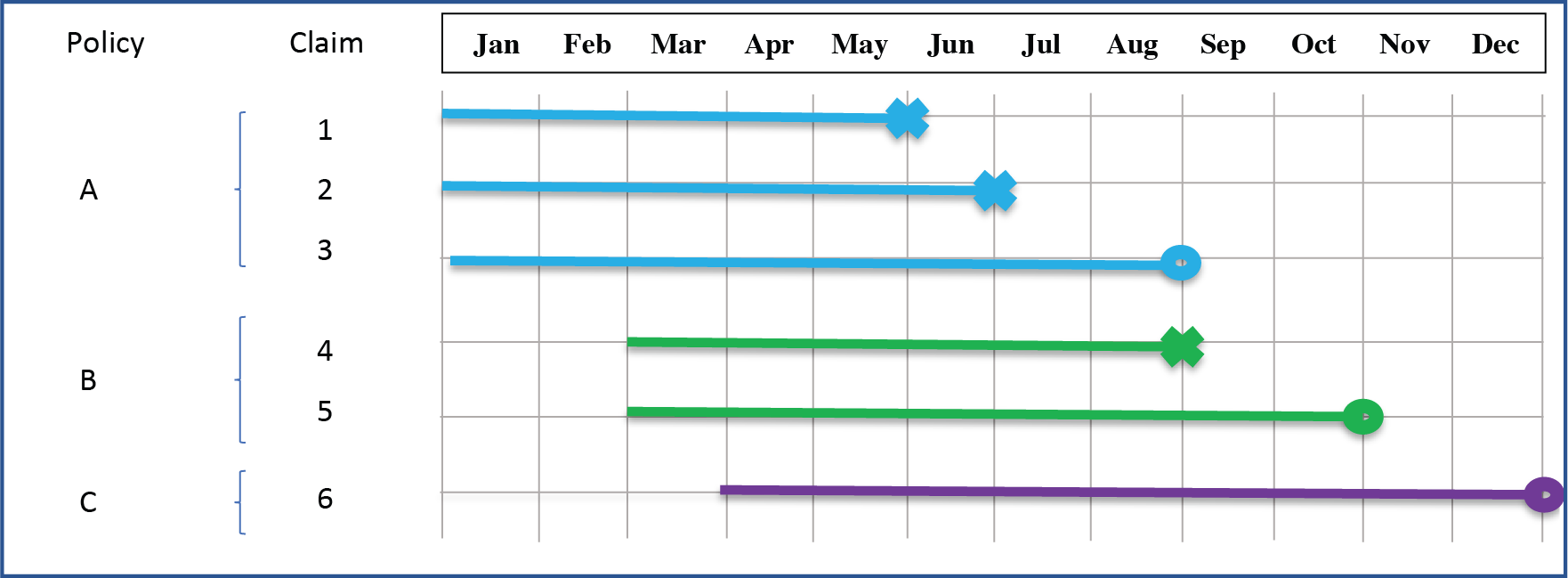
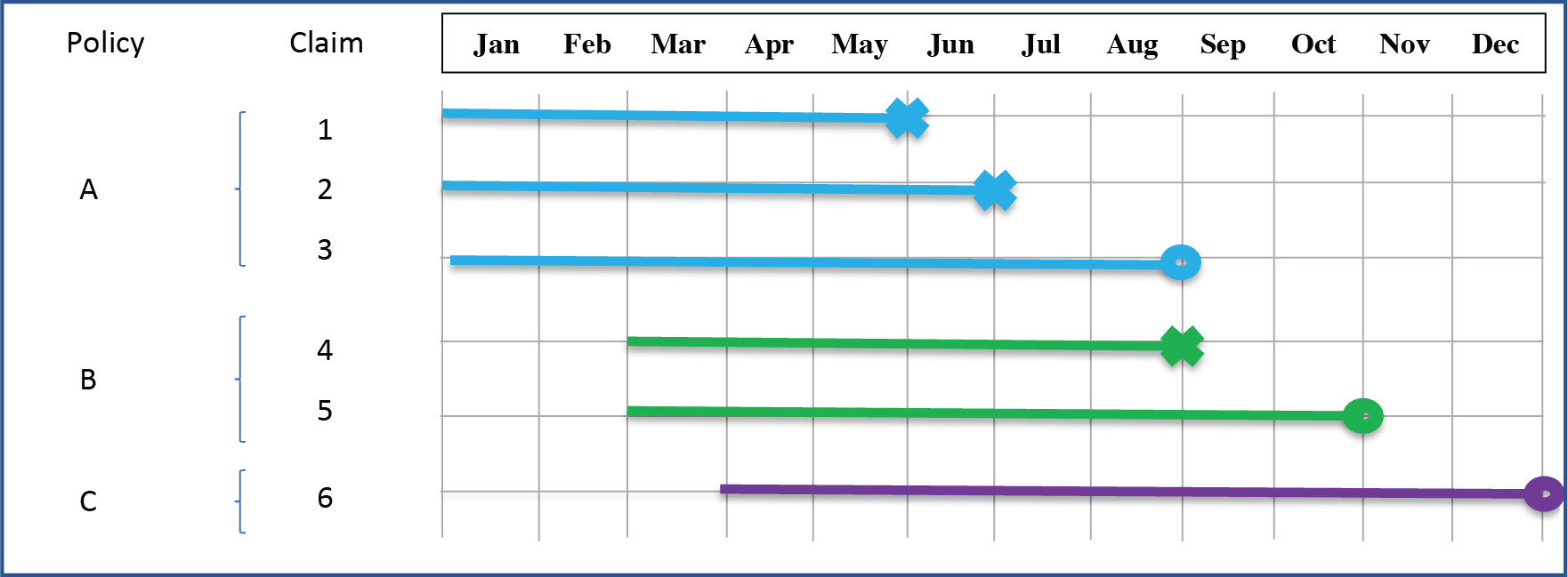
An example of data prepared for the marginal model is presented in Figure 1.

• Policy A starts before January; there are two claims that happened in May and June; policy ends in August.

• Policy B starts in March; there is one claim in August; policy is canceled in October.

• Policy C starts in April; there are no claims in the observed period of time.

Figure 1.Claims data presentation

For this example, data is presented as shown in Table 1.

This case study performs analysis and modeling on claims data for Illinois. The Illinois data contains claims for Consulting, Entertainment, Finance, Hospitality, Manufacturing, Retail, and Utilities industries.

In our analysis, we assume that each claim event is independent within the policy and the industry. For example, if two claims are covered by the same policy, we consider these claims independent. In addition, if two claims are covered by different policies, we assume that the claims are independent and that the policies have no effect on risk. The data for each policy with multiple claim events is described as multiple claims, where each claim has an entry time at the beginning of the policy or beginning of the observation period, whichever is later.

6. Cox model assumptions validation

In most insurance risk papers, the authors take the proportional hazard assumption for granted and make no attempt to check that it has not been violated in their data. That, however, is a strong assumption indeed (Gill and Schumacher 1987). Note that, when used inappropriately, statistical models may give rise to misleading conclusions. Therefore, it’s highly important to check underlying assumptions.

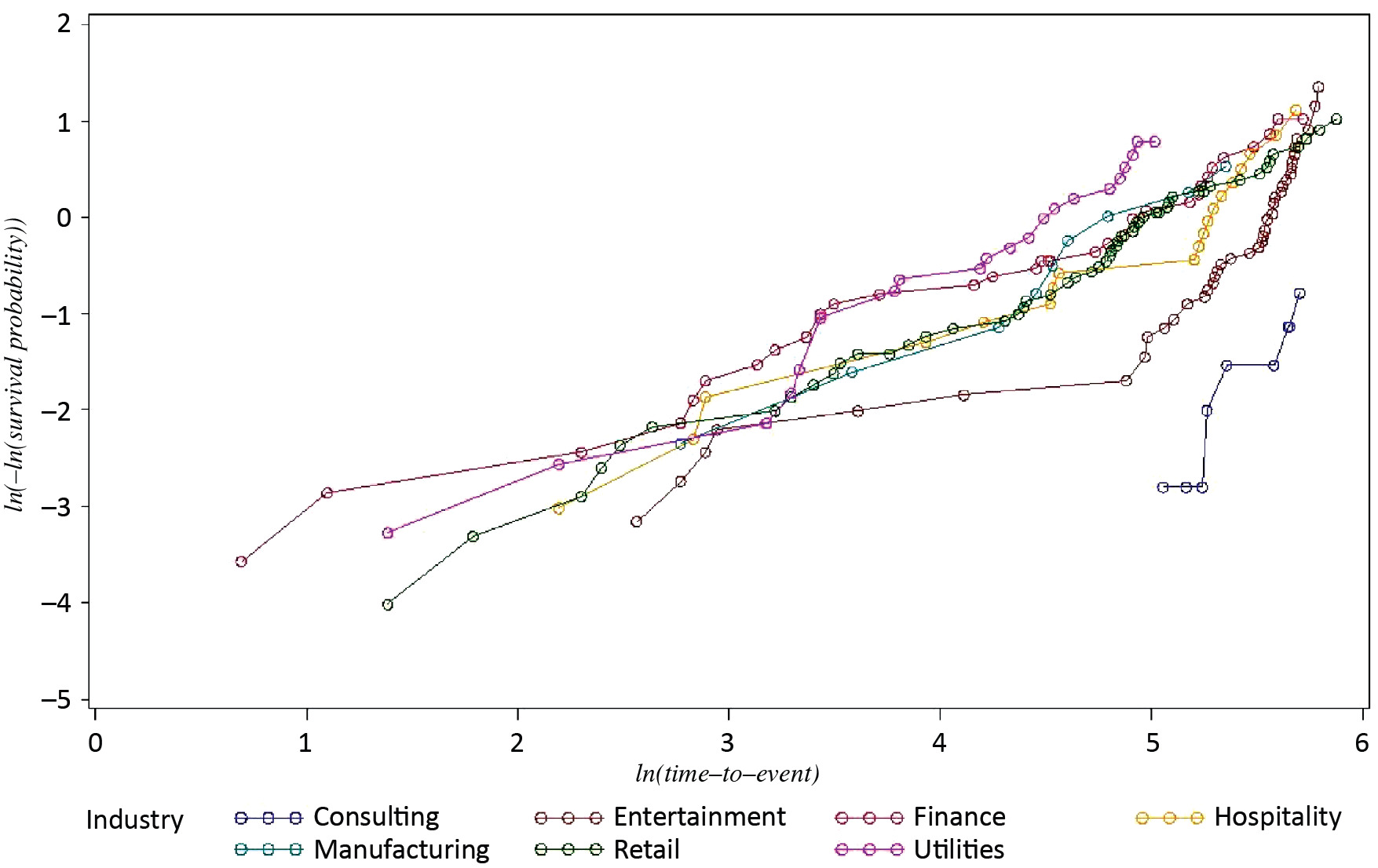
Perhaps the easiest and most commonly used graphical method for checking proportional hazard is the so-called “log-negative-log” plot (Arjas 1988). For this method, one should plot ln(−ln(S_i(t))) vs. ln(t) and look for parallelism—the constant distance between curves over time. This can be done only for categorical covariates. If the curves show a non-parallel pattern, then the assumption of proportional hazard is violated, and, as a result, the analytical estimation of β coefficients is incorrect.

For claims in seven industries in Illinois, the log-negative-log plot is presented in Figure 2. This plot shows that the proportional hazard model assumption does not hold: the lines of the log-negative-log plot are not parallel, and intersect.

Figure 2.Log-negative-log plot for Illinois

We use industry as a categorical covariate, assuming that time-to-event (survival) functions vary by industry. It is wrong to assume that there is no impact on the baseline hazard function for different values of this covariate variable. For example, hazard changes for Retail depend on seasons, or Utilities depend on weather, or Hospitality and Entertainment depend on school breaks schedule.

All these conditions are latently depending on time, which means that the impact of the industry categorical variable does not remain constant over time, thus violating the assumptions of the Cox model. In order to account for season dependency, we introduce a time-dependent covariate for the winter season, and use an extended Cox model:

$$h_{i}(t)=h_{0}(t) \exp \left(\sum_{j=1}^{k} \beta_{j} x_{i j}+\sum_{n=1}^{m} \gamma_{n} x_{i n} g_{n}(t)\right)$$

where:

1. h_i(t) – the hazard function for subject i at time t

2. x₁, . . . , x_k – the covariates

3. h₀(t) – the baseline hazard function that is the hazard function for the subject whose covariates x₁, . . . , x_k all have values of 0

4. g_n(t) – the function of time (time itself, log time, etc.)

5. β₁, . . . , β_k – the coefficients of the Cox model

6. γ_n – the coefficients of time-dependent covariates in the extended Cox model.

Applying this approach to the case of Illinois, our model looks like:

$$h_{i}(t)=h_{0}(t) \exp \left(\sum_{j=1}^{6} \beta_{j} x_{j}+\gamma \times \text { season } \times \ln (t)\right)$$

where

1. h_i(t) – the hazard function for industry i = 1, . . . , 6 at time t, where industries are: Consulting, Entertainment, Finance, Hospitality, Manufacturing, and Retail

2. h₀(t) – the baseline hazard function, in our case—the hazard function for one selected industry, by default, the last alphabetically ordered industry − Utilities.

3. $x_{j}=\left\{\begin{array}{ll} 1, & \text { if } i=j \\ 0, & \text { if } i \neq j \end{array}\right.$

4. $\text { season }=\left\{\begin{aligned} 1, & \begin{array}{l} \text { if the claim happened during } \\ \text { winter season (November 1st - } \\ \\ \text { March 31st) } \end{array} \\ 0, & \begin{array}{l} \text { if the claim happened during } \\ \text { non-winter season (April } 1 \text { st - } \\ \text { October } 31 \text { st) } \end{array} \end{aligned}\right.$

5. γ – the coefficient of the time-dependent covariate

As there is no reason to prefer any specific industry for a baseline, we choose the last alphabetically ordered industry, Utilities. The selection of the Utilities industry as a baseline for hazard means that hazards for all other industries are estimated relative to that of the Utilities industry.

Calculation of time-to-event (survival) functions when we have time-varying covariates becomes more complicated because we need to specify a path or trajectory for each variable. For example, if a policy started on April 01, survival function should be calculated using hazard corresponding to season = 0 for time-to-event t ≤ 214 days (from April 01 till November 01), while for time-to-event t > 214, using hazard corresponding to season = 1. For another example, if a policy started on August 01, survival function should be calculated using hazard corresponding to season = 0 for time-to-event t ≤ 92 days (from August 01 till November 01), and t > 244 days (from April 01 till July 31), while for time-to-event 92 < t ≤ 244, using hazard corresponding to season = 1.

Unfortunately, the simplicity of calculation of S_i(t) is lost: we can no longer simply raise the baseline survival function to a power. For our model, we develop an appropriate formula for the calculation of S_i(t):

$$\begin{aligned} S_{i}(t)= & \left(\frac{S_{0}\left(t \mid t<t_{1}\right) S_{0}\left(t \mid t>t_{2}\right)}{S_{0}\left(t \mid t_{1} \leq t \leq t_{2}\right)}\right)^{\exp \left(\sum_{j-1}^{k} \beta_{j} x_{i j}\right)} \\ & * \exp \left(-\exp \left(\sum_{j=1}^{k} \beta_{j} x_{i j}\right) * \int_{t_{1}}^{t \mid t_{1} \leq t \leq t_{2}} h_{0}(u) u^{\gamma} d u\right) \end{aligned}$$

where:

1. t₁ – the start day of the winter season relative to the beginning of the policy

2. t₂ – the end day of the winter season relative to the beginning of the policy

Another challenge in our data is the reliability of dates related to claims. There are two dates available, the date of the accident that caused the claim, and the date when the claim was reported. The wide variability of time intervals between these two dates creates an additional challenge in the application of the Cox hazard model. To address these problems, as well as assumptions violations, we use a Bayesian nonparametric approach to estimate the coefficients of the extended Cox hazard model (Kalbfleisch 1978).

7. Bayesian approach

The Bayesian approach is based on a solid theoretical framework. The validity and application of the Bayesian approach do not rely on the proportional hazards assumption of the Cox model, thus, generalizing the method to other time-to-event models and incorporating a variety of techniques in Bayesian inference and diagnostics are straightforward (Ibrahim, Chen, and Sinha 2005). In addition, inference doesn’t rely on large sample approximation theory and can be used for small samples. In addition, information from prior research studies, if available, can be readily incorporated into the analysis as prior probabilities. Although choosing prior distribution is difficult, the non-informative uniform prior probability is proved to lead to proper posterior probability (Gelfand and Mallick 1994). Instead of using partial maximum likelihood estimation in the Cox hazard model, the Bayesian method uses the Markov chain Monte Carlo method to generate posterior distribution by the Gibbs sampler: sample from a specified prior probability distribution so that the Markov chain converges to the desired proper posterior distribution. However, a known disadvantage of this method is that it is computation intensive.

8. Deployment with SAS software

To estimate coefficients of the Cox hazard model, we use SAS software, specifically the PHREG procedure, which performs analysis of survival data. The estimation of the Cox hazard model using a Bayesian approach by SAS PROC PHREG is implemented in the following way:

proc phreg data= CLAIMS_DATA_IL; 
class CLIENT_INDUSTRY; 
model TIME_TO_EVENT*CENSOR(0) = 
  CLIENT_INDUSTRY SEASON_EVENT; 
SEASON_EVENT = SEASON*log(TIME_TO_EVENT); 
bayes seed = 1 outpost = POST; 
run;

CLAIMS_DATA_IL is an SAS dataset that contains data for the state of Illinois such as industries, time intervals from the beginning of policies to date of claims, etc. The sample of rows from CLAIMS_DATA_IL is presented in Table 2. CLIENT_INDUSTRY column contains names of industries to which claims are related. TIME_TO_EVENT column contains the number of days to an event calculated starting from the beginning of the observation period or from the beginning of the policy, whichever happens later. CENSOR column indicates if the event is a claim (CENSOR=1), or if the event is the end of a policy (CENSOR=0). SEASON column indicates if the event happened during the winter season (SEASON=1) or not (SEASON=0).

There are two covariates in the model: CLIENT_INDUSTRY and SEASON_EVENT. CLIENT_INDUSTRY is a categorical variable, so it is defined as the covariate in the CLASS statement and the MODEL statement. SEASON_EVENT is the time-dependent covariate that represents the following component of the model: season × ln(t). SEASON_EVENT is defined in the MODEL statement and in the expression that follows the MODEL statement.

class CLIENT_INDUSTRY; 
model TIME_TO_EVENT*CENSOR(0) = 
  CLIENT_INDUSTRY SEASON_EVENT; 
SEASON_EVENT = SEASON*log(TIME_TO_EVENT);

The BAYES statement requests a Bayesian analysis of the model by using Gibbs sampling.

In the BAYES statement, we specify a seed value as a constant to reproduce identical Markov chains for the same input data. We didn’t specify the prior distribution, thus applying uniform non-informative prior.

The described PHREG procedure produces an estimation of β and γ coefficients.

However, PROC PHREG does not produce baseline survival function S₀(t) when the time-dependent covariate is defined. To calculate the baseline survival function, we use the following workaround (Thomas and Reyes 2014):

data DS; 
set CLAIMS_DATA_IL; 
SEASON_EVENT = SEASON*log(TIME_TO_EVENT); 
run;

data INDUSTRY; 
CLIENT_INDUSTRY = "Utilities"; 
SEASON_EVENT = 0; 
run; 

proc phreg data=DS; 
class CLIENT_INDUSTRY; 
model TIME_TO_EVENT *censor(0) = 
  CLIENT_INDUSTRY SEASON_EVENT; 
bayes seed=1; 
baseline out = BASELINE survival = 
  S covariates = INDUSTRY; 
run;

This step produces baseline survival function S₀(t).

9. Interpretation of results

Estimations of β coefficients of the Cox model for each industry except Utilities are presented in Table 3. Because the Utilities industry is used as a baseline for hazard, the β coefficient for Utilities is equal to 0. Table 3 also contains the γ coefficient for SEASON_EVENT covariate.

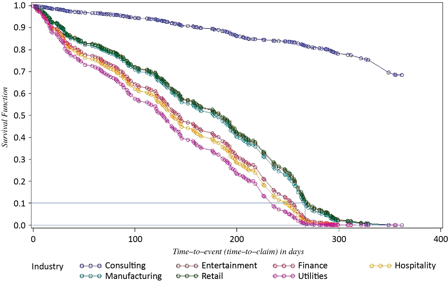
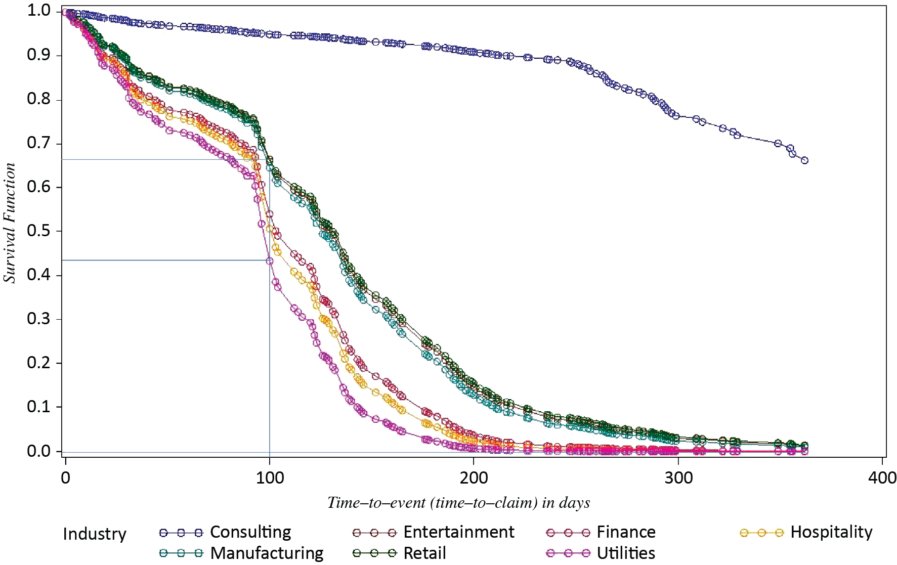
For the purposes of comparing the risk of claims for different industries, we build survival functions for each industry, and season = 0 (Figure 3). According to the survival function for the Utilities industry, for example, there is a 58% chance that there will be no claims before the 100th day of policy, and there is a 1% chance that there will be no claims at all for a one-year policy.

Figure 3.Survival functions for industries in Illinois

The survival functions allow to estimate and to compare the risk of claims among industries. For example, for the Entertainment industry, there is a 72% chance that there will be no claims before the 100th day of policy, and a 5.9% chance that there will be no claims at all for a one-year policy. In other words, the Entertainment industry in Illinois presents a 4.9% higher chance than the Utilities industry to have no claims during a one-year policy. Also, we can observe that Entertainment, Manufacturing, and Retail have very similar risks of claims in Illinois. In addition, there is strong evidence that the Consulting industry has significantly lower risk than other industries.

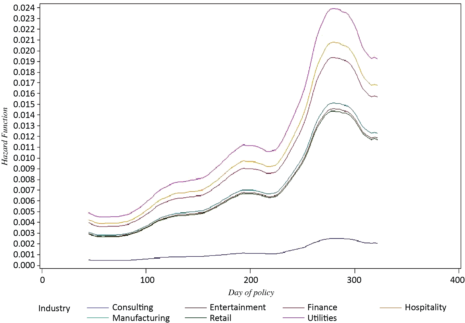
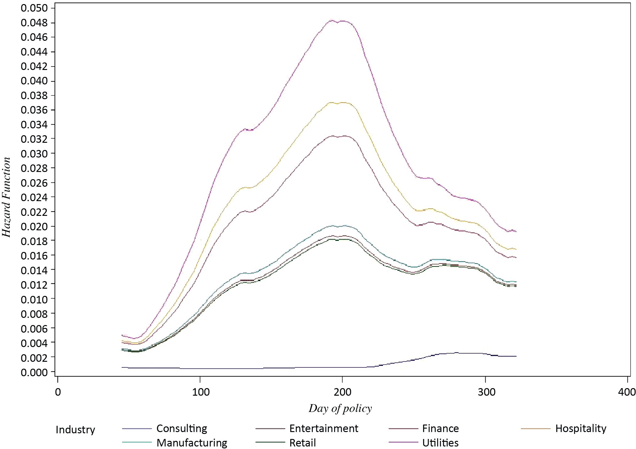
The hazard function presented in Figure 4 shows that the instantaneous claims rate continuously increases, achieving the highest claims rate around the 280th day of policy, and then slightly decreasing. We can also observe that the Consulting industry has a somewhat constant and relatively low claims rate through the duration of a policy. The hazard function in Figure 4 was produced with the SMOOTH SAS macro program (Allison 2012).

Figure 4.Hazard function (instantaneous claims rate per day) for industries in Illinois

Time-dependent covariate SEASON_EVENT is significant with γ = 0.277 . This means that hazard ratio during the winter season in Illinois is 32% higher, controlling for the other covariates:

$$\exp (0.277)-1 \approx 0.32=32 \% .$$

Estimation of survival (time-to-event) function for a specific policy should take into consideration when the policy started—and thus when chances of claims increase due to the winter season.

Calculation of survival functions when we have time-varying covariates is not straightforward, because we need to specify exactly when a specific policy started, and when, relative to the start date of the policy, the winter season occurred. A proprietary computer program has been developed by the authors to calculate S_i(t) for each industry with the time-dependent covariate.

Below we compare two examples mentioned earlier: the case when the policy started on April 01 and the case when the policy started on August 01.

If a policy started on April 01, then during time t ≤ 214 days (from April 01 till November 01) season = 0. Then, for the duration of time t > 214 days till the end of the policy, season = 1. Thus, survival function is calculated using hazard corresponding to season = 0 for time-to-event t ≤ 214 days, and for time-to-event, t > 214 using hazard corresponding to son = 1. The survival function for this case is presented in Figure 5.

Figure 5.Survival function for industries in Illinois with SEASON_EVENT time covariate, and policy starting on April 01

In comparison with Figure 3, where the winter season was not taken into consideration, we can see that the proportion of survival drops staring from the 214th day of the policy.

Both Entertainment and Utilities industries have a 0% chance that there will be no claims at all for a one-year policy when we take the winter season into consideration.

In fact, for the Utilities industry, there is a 0% chance that there will be no claims even before the 270th day of the policy. However, the chances that Entertainment will “survive” without claims by the 270th day are about 10%.

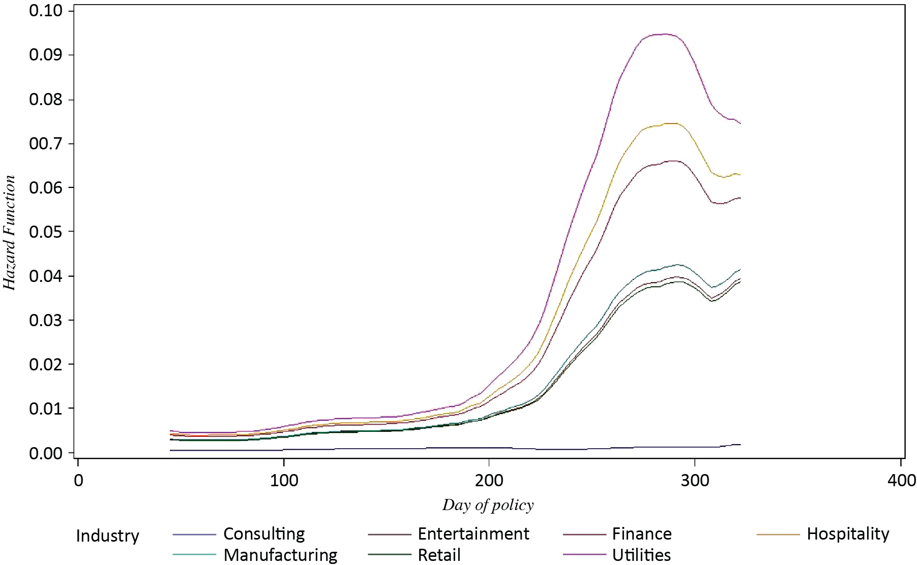
Hazard function presented in Figure 6 shows that the instantaneous hazard of claims sharply increases after t > 214, achieving highest claims rate around the 280th day of a policy term.

Figure 6.Hazard function for industries in Illinois with SEASON_EVENT time covariate, and policy starting on April 01

For the second example, if a policy started on August 01, then during time t ≤ 92 days (from August 01 till November 01) and t > 244 days (from April 01 till July 31), season = 0. Then, for the duration of time 92 < t ≤ 244 days of the policy, season = 1. Thus, survival function is calculated using hazard corresponding to season = 0 for time-to-event t ≤ 92 and t > 244 days, and for time-to-event 92 < t ≤ 244 using hazard corresponding to season = 1. The survival function for this case is presented in Figure 7.

Figure 7.Survival function for industries in Illinois with SEASON_EVENT time covariate, and policy starting on August 01

In comparison with Figure 3, where the winter season was not taken into consideration, we can see that the proportion of survival drops before the 100th day of the policy.

For the Utilities industry, there is a 43% chance that there will be no claims before the 100th day of a policy accounting for winter season vs. 58% without accounting for the winter season. After that, the chance decreases, and by the 210th day of the policy, there is a 0% chance that there will be no claims in the Utilities industry, accounting for the winter season.

For the Entertainment industry, there is a 67% chance that there will be no claims by the 100th day of a policy when we take winter season in consideration, vs. 72% otherwise. Also, there is about 1% chance that there will be no claims at all for a one-year policy—in comparison with a 5.9% chance when we don’t take the winter season into consideration.

The hazard function presented in Figure 8 shows that the instantaneous hazard of claims sharply increases around the 100th day of policy, achieving the highest claims rate between the 180th and 200th day of a policy term.

Figure 8.Hazard function for industries in Illinois with SEASON_EVENT time covariate, and policy starting on August 01

The information revealed by the presented models can be used for purposes of underwriting and pricing for the development of new insurance products, as well as for marketing. For example, insurers can estimate the risk of claims more accurately depending not only on the industry, but also on the time period when the policy is started. Insurers can better manage anticipation of losses related to claims. In addition, insurers can develop new workers’ compensation products for a duration shorter than one year. In this case, the insurance during periods of lower risk will have a lower premium and, therefore, higher acceptance rate by customers. Referring to the example when a policy starts on April 01, a six-month policy would have significantly lower risk and will justify lower premiums. The marketing of such new products will attract companies seeking workers’ compensation.

10. Summary

An ultimate goal of insurance risk assessment is to create a profitable portfolio and to fit the right price to the right risk. This complex problem comprises from multiple parts, including estimation of risk, estimation of price, monitoring of market changes, and more. In our paper, we discussed one part of this complex problem—estimation of risk of workers’ compensation claims for different industries and states with season-dependent factor. Our method to estimate hazard function using a Bayesian approach allows estimating the risk of claims per industry and state, ranking industries by risk within states, as well as estimate risk depending on time-varying covariates like a season. As a next step to build a profitable portfolio, the severity of claims should be included in the analysis, which eventually will allow re-evaluating premiums and insurance products to increase the profitability of portfolios.