


1. Introduction
The estimation of outstanding claims liabilities is one of the central problems in general insurance. Many techniques exist to carry out this task—for example, the chain ladder in its various forms, payments per claim models, and case estimate models. A good review of existing methods is given in Taylor (2000).
Taylor (2000) also discusses a state space model, the Kalman filter (Kalman 1960), which was introduced into the actuarial literature by De Jong and Zehnwirth (1983). This is a recursive algorithm, commonly run by accident or calendar year, which, when applied to the modeling of outstanding claims liabilities, permits the model parameters to evolve over time.
Although a very flexible tool, the Kalman filter requires the assumption of normally distributed data. In the context of loss reserving, this is generally dealt with by assuming that the variables of interest (claim sizes, payments in a specific period, etc.) are lognormally distributed. Although a common assumption in the actuarial field [see, e.g., England and Verrall (2002)], this is an approach not without its problems. The main difficulty is the requirement for a bias correction which results from modeling a transformation of the data (in this case log(payments)), the determination of which, particularly when the distribution of the data is only approximately known, can be problematic. A second drawback is the restriction to one possible distribution for the data. Modeling claim counts, for example, would not be easily done with either a normal or lognormal distribution.
An alternative family of distributions that is worth considering is the exponential dispersion family (termed “EDF” within this paper). This family was introduced by Nelder and Wedderburn (1972) and is treated in depth by McCullough and Nelder (1989). The family includes common distributions like the normal, Poisson, gamma, and inverse Gaussian. The gamma distribution, and to a lesser extent, the inverse Gaussian distribution, are both candidates for the modeling of long-tailed, strictly positive variables. The Poisson distribution is a natural choice for claim counts. Applied within the framework of a filter, this would mean updating a generalized linear model (McCullough and Nelder 1989) rather than a normal linear model (the Kalman filter).
In general, updating a GLM is analytically intractable unless some very restrictive assumptions are made [see, e.g., West, Harrison, and Migon (1995)]. However, putting the problem into a Bayesian context, where the parameter estimates and distribution from the previous application of the filter form the prior distribution of the current step of the filter, it may be seen that the problem is amenable to modeling using Markov Chain Monte Carlo techniques [see, for example, Hastings (1970); Smith and Roberts (1993); Tierney (1994)]. Examples of MCMC in the actuarial literature appear in Scollnik (2001, 2002b), Nzoufras and Dellaportas (2002) and de Alba (2002). Indeed, Nzoufras and Dellaportas (2002) discuss the application of MCMC to some state space models, the implementation of which is further discussed in Scollnik (2002a).
However, MCMC simulation is a time-consuming process, with pitfalls for the unwary user (primarily convergence issues). It would be advantageous to have an analytical version for members of the exponential disperson family corresponding to the Kalman filter. Taylor (2008) derives a second order approximation to the posterior likelihood of a naturally conjugated generalized linear model (GLM). This family of second order approximations is forced to be closed under Bayesian revision. This is a useful finding since it means that the process may be used recursively, i.e., it may be used to form an adaptive filter, which may be used in the modeling of claims data.
Results from an adaptive filter may be used to generate central estimates of an outstanding claims liability. In general insurance practice, other moments are important, in particular the variance of the reserve as well as certain quantiles (e.g., 75%, 95% points). It is possible to use bootstrapping (e.g., Efron and Tibshirani 1993) to yield such information from an adaptive filter. However, standard forms of bootstrapping as applied to actuarial data [see, for example, Taylor (2000)] assume that the residuals are independent. Residuals that result from an adaptive filtering process are, in fact, not independent. Thus, it is necessary to adapt an approach similar to that outlined in Stoffer and Wall (1991) for normally distributed state space models.
Since adaptive filtering, even with bootstrapping, is much quicker than MCMC, it is practical to apply several different models to one data set. These allow the capture of different aspects of the claims experience. To produce a final answer, it is necessary to produce a blended version of all the models. One possible approach is presented in Taylor (2000).
The purpose of this paper is to demonstrate the use of the application of Taylor’s (2008) GLM adaptive filter, incorporating the calculation of central estimates, the application of bootstrapping, and the blending of results from several models to produce a final result. In the remainder of the paper, the data are described in Section 2, while Section 3 introduces the methodology underlying the GLM adaptive filter. This discussion encompasses adaptive filter methodology, an appropriate form of bootstrap for such filters, and means for blending the results from several models. The various models applied to the data are described in Section 4. Section 5 presents some numerical results. The paper closes with some discussion in Section 6.
2. Data
The data used in this paper, from a bodily injury liability portfolio, were summarized as follows:
-
Total amount of claim payments for year of accident i (i = 1, 2, . . . , 14) and development quarter j (j = 1, 2, . . . , 53)
-
Total number of claims reported for year of accident i and development quarter j
-
Total number of claim closures for year of accident i and development quarter j
-
Total amount of case estimates for year of accident i and development quarter j
The data were split into two groups by legal jurisdiction, and each of the above summaries was available for each of these two groups.
Ultimate numbers of incurred claims by accident year were also available; these had been estimated in a separate modeling exercise.
The payments and case estimate data were adjusted for past economic inflation in line with an appropriate wage earning index.
Some notation is defined here. Let
-
CijL = claim payments in development quarter j for accident year i for jurisdictional grouping L (L = 1, 2);
-
NijL = number of claims reported in development quarter j for accident year i for jurisdictional grouping L;
-
FijL = number of claim closures in development quarter j for accident year i for jurisdictional grouping L;
-
EijL = case estimates at end of development quarter j for accident year i for jurisdictional grouping L;
-
UiL = estimated ultimate number of claims incurred in accident year i for jurisdictional grouping L; and
-
OijL = number of claims open for accident year i, at start of development quarter j for jurisdictional grouping L.
3. Methodology
This section opens with a discussion of the Kalman filter and outlines the generalization to the analytical GLM filter developed by Taylor (2008). It then describes the adaptation of the Stoffer and Wall (1991) bootstrap required for GLM filters. Finally, the blending methodology is described.
3.1. Kalman filter
Following Taylor’s (2000) description, the model underlying the Kalman filter consists of two equations, called the system equation and observation equation. The former describes the model’s parameter evolution, while the latter describes the model of observations conditional on the parameters. The two equations are as follows:
System equation
β(s+1)=Φ(s+1)p×1β(s)p×p(s)p×1+r(s+1)p×1.
Observation equation
Y(s+1)=X(s+1)n×1(s+1)n×p(s+1)p×1+v(s+1)n×1.
These equations are written in vector and matrix form with dimensions written beneath, and
-
Y(s + 1) denotes the vector of observations made at time s + 1 (= 1, 2, . . . T).
-
β(s + 1) denotes the vector of parameters at time s + 1.
-
X(s + 1) is the design matrix applying at time s + 1.
-
Φ(s + 1) is a transition matrix governing the evolution of the expected parameter values from one epoch to the next.
-
r(s + 1) and v(s + 1) are stochastic perturbations, each with zero mean, and with
Var[r(s+1)]=R(s+1) and Var[v(s+1)]=V(s+1).
The Kalman filter is an algorithm for calculating estimates of the β(s + 1). It revises the parameter estimates iteratively over time. Each iteration introduces additional data Y(s + 1). Specific details of its application to loss reserving may be found in Taylor (2000).
The formal statement of the filter requires a little extra notation. Let Y(s | s − k) denote the filter’s estimate of Y(s) on the basis of information up to and including epoch s − k; and similarly for other symbols at s | s − k. Also, let Θ(s | s − k) denote the estimate of Var[β(s | s − k)].
Equations (3.4) through (3.8) present the mathematical detail behind the Kalman filter. The process may be split into four steps.
Step 1
β(s∣s−1)=Φ(s)β(s−1∣s−1)
Θ(s∣s−1)=Φ(s)Θ(s−1∣s−1)ΦT(s)+R(s)
Step 2
L(s∣s−1)=X(s)Θ(s∣s−1)XT(s)+V(s)
K(s)=Θ(s∣s−1)XT(s)[L(s∣s−1)]−1.
Step 3
ˆY(s∣s−1)=X(s)β(s∣s−1).
Step 4
β(s∣s)=β(s∣s−1)+K(s)(Y(s)−ˆY(s∣s−1))
Θ(s∣s)=(1−K(s)X(s))Θ(s∣s−1).
Equations (3.4) to (3.8) generate forecasts of the new epoch’s parameters and observations based on no new information. The gain matrix (credibility of the new observation) is calculated in Equation (3.7). Finally the parameter estimates are updated in Equations (3.9) and (3.10). The process then moves on to the next epoch, starting again with Equation (3.4).
The filter starts with prior estimates for β(0 | 0) and the associated dispersion Θ(0 | 0).
The key equation for revising parameter estimates is Equation (3.9). The main characteristics of this formula are that:
-
It is linear in the data vector Y(s).
-
β(s | s) is the Bayesian revision of the estimate of β(s − 1 | s − 1) in the case that r(s) and v(s) are normally distributed.
-
Consequently, K(s) is equivalent to the credibility of Y(s).
The Kalman filter is a form of an adaptive filter—a form of time series estimation in which parameter estimates are constructed so as to track evolving parameters.
3.2. Exponential dispersion family
The exponential dispersion family (EDF) (Nelder and Wedderburn 1972) is a large family of distributions of varying tail length. This paper uses a slightly restricted version of the family whose members have a likelihood of the following form:
L(y∣θ,λ)=a(λ,y)expλ[yθ−b(θ)]
where θ, λ are parameters and a(.) and b(.) are functions characterizing the members of the family. The more general form of EDF allows λ to be a function λ(φ) of a dispersion parameter φ rather than a constant.
It may be shown that, for the distribution defined in Equation (3.11),
E[Y∣θ,λ]=b′(θ), and Var[Y∣θ,λ]=b′′(θ)/λ
Denote b′(θ) by μ(θ) whence, provided that μ(.) is one-one
Var[Y∣θ,λ]=V(μ(θ))/λ
for some function V(.) called the variance function.
Many applications of the EDF restrict the form of the variance function to
V(μ)=μp
for some constant p ≤ 0 or p ≥ 1. This family is referred to as the Tweedie family (Tweedie 1984). The likelihoods corresponding to such a restriction will be referred to below as EDF(p).
Some special cases of the EDF are:
-
p = 0: normal
-
p = 1: Poisson
-
p = 2: gamma
-
p = 3: inverse Gaussian
A further quantity associated with the EDF is the scale parameter. This is given by
φ=1/λ.
3.3. Analytical GLM filter
Taylor (2008) examined the problem of finding closed-form solutions to the Bayesian revision problem for GLMs. That paper builds on the univariate case where the exponential dispersion family is closed under Bayesian revision in the presence of natural conjugate priors. Although this is not the case for the general multivariate EDF, Taylor (2008) derives a second order approximation to the posterior likelihood of a naturally conjugated GLM. This family of second order approximations is forced to be closed under Bayesian revision. This is a useful result since it means that the process may be used recursively, i.e., it may be used to form an adaptive filter, thereby allowing a model to adapt to changing experience.
Although Taylor (2008) gives a general form of the filter, he notes that it is only analytically tractable in a limited set of cases, in particular where the link function corresponds to either the canonical or companion canonical link (as defined within the paper). Tractable cases include the Poisson distribution with log link and the gamma distribution with reciprocal link (canonical link) or log link (companion canonical link). This filter is termed the analytical GLM filter (or GLM filter for short) in this paper. The filter implements a dynamic generalized linear model, i.e., a GLM in which parameters vary over time.
Note also that the normal distribution with identity link is also a member of this class of filters; Taylor (2008) shows that this is exactly equal to the Kalman filter. In other words, the second order approximations used in that paper become exact in the case of the normal distribution and an identity link.
Full details of the general form of the filter as well as some specific examples are available in Taylor (2008). However, since the cases of gamma error/log link (companion canonical link) and the Poisson error/log link (canonical link) versions of the filter will be used extensively in this paper, the series of equations defining this filter is given here.
3.3.1. The gamma GLM filter
The equations underlying the analytical GLM filter follow the Kalman filter, in principle, but are considerably more complex. Below, the key definitions and equations for the gamma GLM filter are given, with supplementary formulae in Appendix A.1. Note that in all the equations below (and those in Appendix A and Appendix B), functions are assumed to operate componentwise on vectors.
The system equation for the analytical gamma GLM filter is the same as that in (3.1). However, the observation equation differs due to the log link and is
Y(s+1)=exp{X(s+1)β(s+1)}+v(s+1)
Some other quantities of importance within the gamma GLM are defined as follows:
1/h−1(s∣s−j)=E[exp{−M(s∣s−j)β(s∣s−j)}]Γ(s∣s−j)=Var[exp{−M(s∣s−j)β(s∣s−j)}]
where M(s | s − j) is defined in Appendix A and s | s − j denotes estimates at epoch s on the basis of information up to and including epoch s − j.
The gamma GLM filter is applied to these quantities, from which the parameter means and variances are estimated. In the case of the Kalman filter, the corresponding expressions in Equations (3.17) simplify to β(s | s − j) and Θ(s | s − j) from Section 3.1.
The equations describing the gamma GLM filter are given below. Where they make reference to matrices not defined in this section, the reader should refer to Appendix A.1 for their definitions.
Step 1
E[β(s∣s−1)]=Φ(s)E[β(s−1∣s−1)]
Var[β(s∣s−1)]=Φ(s)Var[β(s−1∣s−1)]ΦT(s)+R(s)
where Φ(s + 1) is the identity matrix in the example of filtering in this paper. Equation (3.19) indicates that the parameter vector at any epoch (accident period) is a deterministic linear transformation and stochastic perturbation of its value at the previous epoch.
Also adopt the following approximations to Equations (3.17):
1h−1(s∣s−1)=[I+12Q(s∣s−1)]×exp{−E[M(s∣s−1)β(s∣s−1)]}
Γ(s∣s−1)=Q(s∣s−1) DIAG ×exp{−2E[M(s∣s−1)β(s∣s−1)]}
where DIAG(.) is an operator that converts the subject vector to a diagonal matrix.
Step2
K(s)=B(s∣s)−1P(s)J(s)G(s)
Step 3
ˆY(s∣s−1)=exp{X(s)β(s∣s−1)}.
Step 4
1/h−1(s∣s)= DIAG exp[−M(s∣s)β(s∣s−1)]×[1−K(s)(Y(s)−ˆY(s∣s−1))]
where 1 represents a vector with all entries 1, rather than the unit matrix
Γ(s∣s)=−D(s)−1B(s∣s)2
E[β(s∣s)]=M(s∣s)T{−log1h−1(s∣s)+12Γ(s∣s)H(−1)(s∣s)21}
Var[β(s∣s)]=M(s∣s)TH(−1)(s∣s)Γ(s∣s)H(−1)(s∣s)M(s∣s)
In (3.26) and (3.27),
H(−1)(s∣s)=DIAGh−1(s∣s)
where h−1(s | s) is the reciprocal of 1/h−1(s | s).
The filter is initialized by setting initial values (i.e., prior values) for E[β(0 | 0)] and Var[β(0 | 0)]. Further, input values are required for Λ(s)—for the gamma distribution, the coefficients of variation of the data Y(s) are the appropriate choice. The R(s) may all be set to a constant matrix.
3.3.2. The Poisson adaptive filter
The Poisson adaptive filter is also used in this paper. It is very similar to the gamma filter. Taylor (2008) discusses the relationship between the two, one based on the canonical link (Poisson/log link) and the other based on the companion canonical link (gamma/log link). The key equations are detailed below with supplementary detail in Appendix A.2.
Step 1
E[β(s∣s−1)]=Φ(s)E[β(s−1∣s−1)]
Var[β(s∣s−1)]=Φ(s)Var[β(s−1∣s−1)]Φ(s)+R(s)
Also define:
h−1(s∣s−1)=[I+12Q(s∣s−1)]×exp{M(s∣s−1)E[β(s∣s−1)]}
Γ(s∣s−1)=Q(s∣s−1) DIAG ×exp{2E[M(s∣s−1)β(s∣s−1)]}.
Step 2
ˆY(s∣s−1)=exp{X(s)β(s∣s−1)}.
Step 3
h−1(s∣s)=exp{M(s∣s)β(s∣s−1)}+P(s)J(s)[Y(s)−ˆY(s∣s−1)]
Γ(s∣s)=D(s)−1B(s∣s)2.
E[β(s∣s)]=M(s∣s)T[log(h−1(s∣s))−12Γ(s∣s){H(−1)(s∣s)2}1]
Var[β(s∣s)]=M(s∣s)TH(−1)(s∣s)Γ(s∣s)×H(−1)(s∣s)M(s∣s)
In Equation (3.36), 1 represents a vector of ones, rather than a unit matrix, while
H(−1)(s∣s)=[DIAGh(s∣s)]−1.
3.4. Bootstrap
The GLM filter yields a central estimate of liability. For many applications, an indication of the uncertainty that is associated with the estimate is also useful.
Variability in a forecast results from a number of sources:
-
Parameter error: sampling error in the parameter estimates;
-
Process error: even if the parameter estimates match their true values, future experience will be subject to disturbance
-
Specification error: the error caused by the model being incorrect
The first two of these may be measured using the bootstrap (Efron and Tibshirani 1993). Broadly speaking, a typical bootstrap application involves repeatedly resampling the data to obtain many pseudo data sets. The filter is run through each and the resulting collection of forecast values (and parameter estimates if desired) forms an empirical estimate of the true distribution of that quantity.
Taylor (2000) and Pinheiro, Andrade e Silva, and Centeno (2003) review the application of bootstrapping to loss reserving problems; since the data in a loss reserving triangle are not, in general, identically distributed, an adjusted version of the bootstrap, based on standardized residuals must be used rather than the traditional bootstrap method of simply resampling data points.
When bootstrapping filtered data, a further complication arises in that the resulting residuals are not independent. The correct way of dealing with such lack of independence was discussed in Stoffer and Wall (1991) in relation to the case of normal distributions, identity links (i.e., the Kalman filter). A similar approach should be applied to GLM filters.
The key concept of the Stoffer and Wall (1991) paper is that dependencies must be allowed for in any bootstrapping process. Following the notation in Section 3.1, they first construct the innovations, defined as follows:
ε(s)=Y(s)−X(s)β(s∣s−1).
The innovations covariance matrix is defined as
X(s)Γ(s∣s−1)XT(s)+V(s)=L(s∣s−1)
By (3.39) and (3.40), the standardized innovations may be calculated as
e(s)=L−1/2(s∣s−1)ε(s).
To carry out one iteration of the bootstrap, the standardized innovations, e(s), s = 1, . . . , T, are sampled T times with replacement (where T is the total number of epochs to which the filter is applied). Note that all components of these es are stochastically independent and equivariant, and, for ε(s) normal, equidistributed as is required for the bootstrap resampling.
To create a bootstrap data set, the standardization of the innovations is reversed using Equation (3.41), leading to pseudo innovations, ε*(s), s = 1, . . . , T. These may then be used in the Kalman filter, in Equation (3.9) in place of Y(s + 1) − Ŷ(s +1 | s). A key point to note is that, since the filter depends on the data only through this equation, there is no need to reconstruct a pseudo data set, as would be the case in typical applications of bootstrapping [see, e.g., Efron and Tibshirani (1993); Pinheiro, Andrade e Silva, and Centeno (2003)].
Apart from the modification to Equation (3.9), the remainder of the Kalman filter equations flow through unchanged for a bootstrap iteration, yielding one set of bootstrapped results. The process may then be repeated a large number of times to yield the bootstrapped estimate of the distribution of the results.
For the analytical GLM filter, Equation (3.39) is replaced with Equation (3.42), below, for the gamma/log link case:
ε(s)=1/h−1(s∣s)−exp{−M(s∣s)β(s∣s−1)},
and Equation (3.43) for the Poisson/log link scenario:
ε(s)=h−1(s∣s)−exp{M(s∣s)β(s∣s−1)}.
There is no simple expression for the innovations covariance matrix corresponding to Equation (3.40) for either case. Instead, these must be calculated using Equations (3.24) and (3.34) to find alternative specifications for Equations (3.42) and (3.43) and then calculating the approximate variance of these terms. Appendix B gives these calculations.
As in Stoffer and Wall (1991), the standardized innovations are resampled T times (where T is the number of epochs in the data) for each bootstrap iteration, yielding ẽ(s), s = 1, . . . , T. Similarly, a pseudo innovation is calculated for each epoch and used in place of Equation (3.24) for gamma/log link and Equation (3.34) for Poisson log link. In the gamma/log case the substitution is
1/h−1(s∣s)=˜ε(s)+ DIAG exp[−M(s∣s)β(s∣s−1)]
where ε̃(s)= L1/2(s | s − 1)ẽ(s) represents the sampled innovation. A similar substitution is made in the Poisson/log link case.
The gamma/log link case requires some additional special handling. This is due to the appearance of the data, Y(s), in Equations (A.7) and (A.9), meaning that, in the bootstrap, pseudo data appears within the calculation of the pseudo sample parameters. This renders the computation of pseudo data self-referencing.
The approach that has been taken here is to:
-
Work through the Equations (A.7) and (A.9).
-
Calculate (3.24) using the pseudo innovations. This yields an initial estimate of 1/h−1(s | s).
-
Calculate the implied value, ß̃(s | s − 1) from the relation 1/h−1(s | s) = exp{−M(s | s) · ß̃(s | s − 1)} (refer to (3.17)).
-
Calculate the implied value, Ỹ(s) as Ỹ(s) = exp{X(s)ß̃(s | s − 1)} (refer (3.23)).
-
Recalculate (A.7) and (A.9) with Ỹ(s) and then carry these effects through the remainder of the filter equations.
Note that, as for the Kalman filter, the pseudo innovations (3.42) and (3.43), after diagonalization and standardization, are stochastically independent and equivariant. However, they may not be equidistributed. For example, Poisson variates with differing means, when standardized, are not equidistributed.
Strictly, this breaches the bootstrap requirement of exchangeability of standardized (and diagonalized) residuals, and so introduces an error into the application of the bootstrap to a GLM. We suppose this error to be slight.
Process error
Process error may be incorporated into the bootstrap results by means of the distribution assumed for the data. Thus, the methodology outlined above leads to a mean value for each cell; a value may then be sampled from the appropriate error distribution (e.g., gamma or Poisson) to incorporate process error.
Output
The ultimate output of a bootstrapping procedure, for an outstanding claims estimation process, is a distribution of the outstanding claims liability. However, the mean of the bootstrap distribution will not, in general, equal the mean estimated from the original data set. The disparity will be caused at least by sampling error arising from the finiteness of the sample forming the bootstrap distribution, and it may arise from other errors such as discussed immediately above.
To correct for this, the user may scale the bootstrap values to match the original estimates. This ensures consistency between the bootstrapped results and the mean (such as, for example, the location of various percentile points) while maintaining the same level of variability.
3.5. Blending of model results
It is common practice in actuarial reserving to apply more than one model to the data with the final estimates being a blend of those from all models. In principle, weights assigned to each model should be high where that model is reliable and low where it is not. Further, it may be desirable to take into account the smoothness of certain quantities as they progress over accident periods—for example, the smoothness of the weights themselves and the smoothness of the ratio of the estimates of liability to case estimates of that liability (call these the “case estimate ratios”).
Note that the notation used in this subsection differs in a couple of respects from that introduced in Section 2. For example C and U have different meanings, within the context of the blending algorithm, from those previously used.
The blending procedure followed here shares a lot of common ground with that described in Chapter 12 of Taylor (2000), which in turn is a modification of a procedure proposed in an earlier paper (Taylor 1985). The principle difference is that smoothness of the case estimate ratios is defined here in terms of their logged values, whereas it is defined in terms of their raw values in the cited work.
The reasoning supporting this is as follows. If Ri denotes the case estimate ratio for accident period i, the sequence {Ri, i = 1, 2, . . . , I} will typically display relatively large values for the highest values of i, but tend to converge to a constant as i → 1.
This will resemble an exponential rather than a linear sequence. If it were precisely exponential, then the sequence {ln Ri} would be linear, and second differences Δ2ln Ri of this sequence would be zero. In this sense, smallness of the Δ2 ln Ri is a reasonable criterion for smoothness of the sequence {Ri}.
An outline of the blending procedure is presented below.
Let i = 1, 2, . . . , I, h = 1, 2, . . . , H denote the estimate of outstanding claims liabilities for model h, for accident period i.
Consider blended estimates from the family of linear combinations of the models:
ˆˆLi=H∑h=1wihˆLih
for deterministic coefficients wih.
Let
ˆLi=(ˆLi1,ˆLi2,…,ˆLiH)T
wi=(wi1,wi2,…,wiH)T
ˆLI×HI=[ˆLT1ˆLT2⋱ˆLTI]
w=[w1w2⋮wI].
Note that L̂ is a block diagonal matrix, i.e., a block matrix with, in this case, a 1 × H block for each entry on the diagonal and zero blocks elsewhere. Let
CHI×HI=Var[ˆL1ˆL2⋮ˆLI].
Let qi be the most recent case estimates for accident year i. Let
Q=diag(q−11,q−12,…,q−1I).
Define the rth order differencing matrix, D, as the (I − r) × I matrix with (i, j) element
\begin{array}{rlrl} d_{i j} & =(-1)^{i+j}\binom{r}{j-i}, & j \geq i, \quad j-i \leq r \\ & =0, \quad \text { otherwise. } \end{array} \tag{3.52}
The procedure requires differencing matrices associated with both the (logged) case estimate ratios (DQ, an (I − r) × I matrix, defined as in Equation (3.52)) and DW which is defined as
\tilde{D}_{W}=\left(\begin{array}{ccc} D^{T} D & & 0 \\ & \ddots & \\ & & D^{T} D \end{array}\right) \tag{3.53}
where D is as defined in Equation (3.52).
A reasonable choice for the level of differencing is second order (r = 2), for both the case estimate ratios and the weights.
Let E be the HI × HI matrix which permutes the components of w as follows:
\left[\begin{array}{c} w_{11} \\ w_{12} \\ \vdots \\ w_{I 1} \\ \vdots \\ w_{I H} \end{array}\right] \rightarrow\left[\begin{array}{c} w_{11} \\ w_{21} \\ \vdots \\ w_{1 H} \\ \vdots \\ w_{I H} \end{array}\right] . \tag{3.54}
Let
R=\log (Q L) \tag{3.55}
and
B=R^{T} D_{Q}^{T} D_{Q} R . \tag{3.56}
Now let
T=E^{T} \tilde{D}_{w} E \tag{3.57}
and
G=C+k_{1} B+k_{2} T \tag{3.58}
which is an objective function that assigns relative weights 1, k1 and k2 to
-
variance of total liability according to the blend of models;
-
smoothness of case estimate ratios (more precisely, ratios of logged estimates to logged case estimates); and
-
smoothness of the weights;
respectively. Values of k1, k2 ≥ 0 are to be chosen by the user, and the choice may be made with the assistance of Taylor (1992) and Verrall (1993).
The weights that minimize this objective function, subject to the constraint that ∑hwih = 1 for each i, are
w=G^{-1} U^{T}\left(U G^{-1} U^{T}\right)^{-1} 1 \tag{3.59}
where
U=\left[\begin{array}{cccc} 1^{T} & & & \\ 1 \times H & & & \\ & 1^{T} & & \\ & 1 \times H & & \\ & & \ddots & \\ & & & 1 \\ & & & 1 \times H \end{array}\right] \tag{3.60}
The matrix U arises here from the constraint that the weights for each accident period must sum to unity.
There is no constraint for the weights to be non-negative in the algorithm above; all that is required is for the weights to sum to one for each accident period. It is possible for the algorithm to lead to large, negative weights balanced by large positive weights. This may be seen as undesirable. Therefore, it is proposed that negative weights be forced to zero, with the remaining positive weights being scaled so that they sum to one.
Further, the definition of C in Equation (3.50) may be based upon variances only rather than the full covariance matrices for each model. Restricting C to be a strictly diagonal matrix (rather than block diagonal—where covariances between different accident periods may be nonzero within a model, but covariances between models are assumed zero) can lead to quite different results. In some cases, these may be judged better by the practitioner.
In practice, both the log and linear versions of the blending algorithm should be considered. The linear version of the algorithm follows the same process as outlined above except that Equations (3.55) and (3.56) are replaced by
A=Q^{T} D_{Q}^{T} D_{Q} Q \tag{3.61}
and
B=\hat{L}^{T} A \hat{L} \tag{3.62}
The version that yields the best results for the problem under consideration should be used.
4. Models applied to data
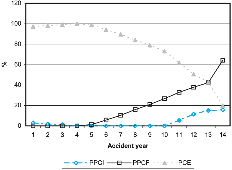
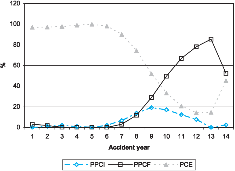
It has been previously indicated that it is customary to consider fitting more than one type of model to claims data when calculating outstanding claims reserves. Three models are considered in this paper, representing to a certain extent the standard repertoire in Australian practice:
-
Payments per claims incurred (PPCI);
-
Payments per claims finalized (PPCF); and
-
Projected case estimates (PCE).
The rationale behind this is that the first two models are payments based. These should perform well where there is a substantial volume of payments (e.g., in early to middle development periods). The PPCF model is particularly suited to claims for which the majority of the payments are made at finalization (and conversely less suited to claims with substantial recurring payments). The PCE model would be expected to perform best in the later development periods. Here, much is known about outstanding claims, so the case estimates would be expected to be reliable.
Definition and discussion of the three models appears in Taylor (2000). Some more detail on each of them follows below. Note that the notation used here is that defined in Sections 2 and 3 (with the exception of Section 3.5).
4.1. Payments per claim incurred model
Let
\mathrm{PPCI}_{i j}^{L}=C_{i j}^{L} / U_{i}^{L} . \tag{4.1}
A commonly used model for PPCIij is the Hoerl Curve (De Jong and Zehnwirth 1983; Wright 1990). This has the following form:
\mu_{i j}=\exp \left\{\beta_{0}+\beta_{1} j+\beta_{2} \log j\right\}, \quad j=1,2, \ldots \tag{4.2}
where μij represents the mean value of PPCIij.
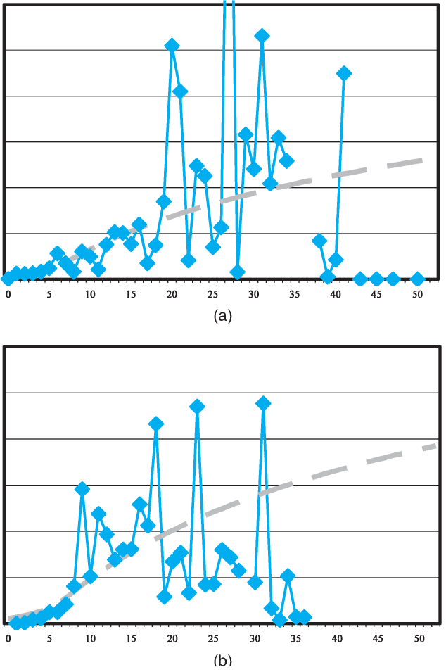
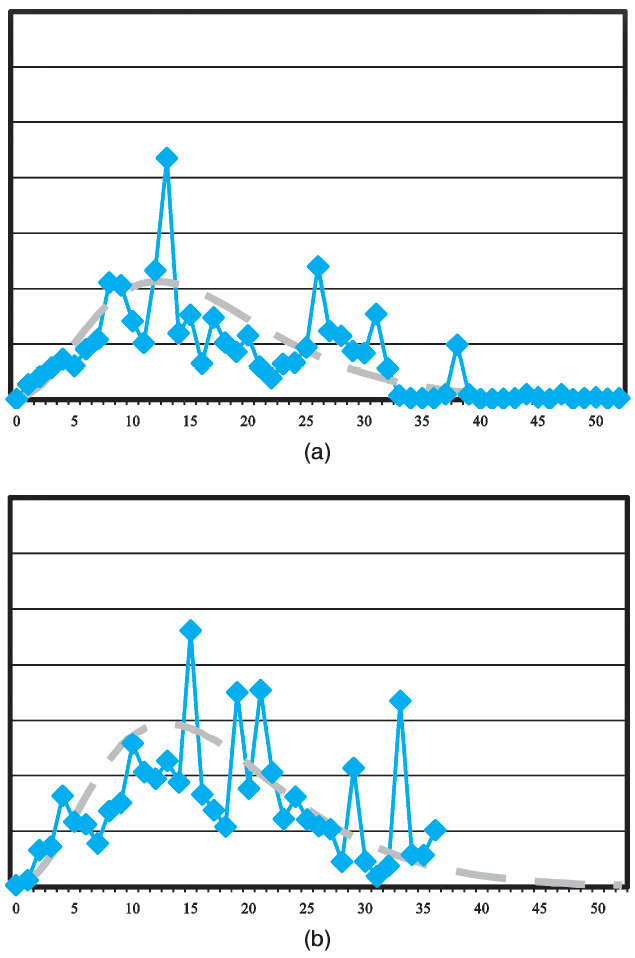
For the particular data set described in Section 2, the Hoerl Curve is used as a starting point and then modified slightly. Further, each jurisdictional group is permitted to have its own shape. The applied model has the form
\begin{aligned} \operatorname{PPCI}_{i j}^{L} \sim & \operatorname{Gamma}\left(\mu_{i j}^{L}, v_{j}\right) \\ \mu_{i j}^{L}= & \exp \left\{\beta_{i 0}+\beta_{i 1} \log j+\beta_{i 2} j+\beta_{i 3} \min (j, 16)\right\} \\ & +\mathrm{I}(L=1)\left\{\beta_{i 4}+\beta_{i 5} \log j+\beta_{i 6} j+\beta_{i 7} \min (j, 16)\right\} \end{aligned} \tag{4.3}
where
-
vj = coefficient of variation in development quarter j; and
-
I(condition) is an indicator function which is 1 if condition is true and 0 otherwise.
The quantity vj may be estimated on the basis of data and actuarial judgment.
Examples of the actual data and fitted model are shown below in Figure 1, which plots PPCIs for one of the jurisdictional groups (labeled as group 0). Note that both graphs are presented on the same vertical scale. Thus, movement in average claim payments from accident year 1 to 5 is apparent in these plots.
4.2. Payments per claims finalized model
The payments per claims finalized model (PPCF) actually consists of two submodels:
-
Average payments per claim finalized;
-
The probability that a claim finalizes in a particular quarter.
Model of average payments per claim finalized
Let
\operatorname{PPCF}_{i j}^{L}=C_{i j}^{L} / F_{i j}^{L} . \tag{4.4}
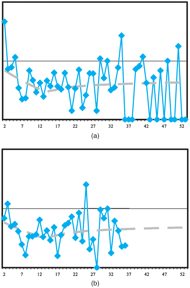
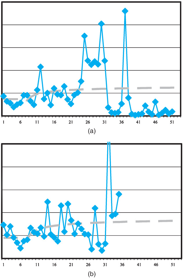
Average payments per finalized claim tend to increase with age of claim since the more complicated and serious claims are more likely to take longer to settle. For the data in this paper, the following model is used:
\begin{aligned} \operatorname{PPCF}_{\mathrm{ij}}^{\mathrm{L}} \sim & \operatorname{Gamma}\left(\mu_{i j}^{L}, v_{j}\right) \\ \mu_{i j}^{L}=\exp \{ & \beta_{i 0}+\mathrm{I}(L=0)\left[\beta_{i 1}\left(\frac{j-1}{4}\right)^{-0.4}\right. \\ & \left.+\beta_{i 2} \min (6, j-1)\right] \\ & +\mathrm{I}(L=1)\left[\beta_{i 3}+\beta_{i 4}\left(\frac{j-1}{4}\right)^{-0.75}\right. \\ & \left.\left.+\beta_{i 5} \min (6, j-1)\right]\right\} \end{aligned} \tag{4.5}
where
-
μijL = the mean PPCFijL in cell (i, j);
-
vj = coefficient of variation in development quarter j; and
modeling begins in the second development quarter (i.e., j = 2).
Examples of the actual data and fitted model are shown in Figure 2. Again, both graphs are presented on the same vertical scale.

Model of probability of finalization
Let
\operatorname{PRF}_{i j}^{L}=F_{i j}^{L} /\left(O_{i j}^{L}+N_{i j}^{L} / 3\right) . \tag{4.6}
The denominator in (4.6) is an exposure measure of the number of claims that may finalized in cell (i, j). The probability of finalization for the data in this paper is quite a volatile quantity; therefore simple models have been used. PRFijL ∼ Overdispersed Poisson (μLij,vj)
\begin{aligned} \mu_{i j}^{L}=\exp \{ & \beta_{i 0}+\mathrm{I}(L=0)\left[\beta_{i 1} \min (j-1,15)\right. \\ & \left.+\beta_{i 2} \max (1, j-13)^{-0.25}\right] \\ & +\mathrm{I}(L=1)\left[\beta_{i 3}+\beta_{i 4} \min (j-1,15)\right. \\ & \left.\left.+\beta_{i 5} \max (1, j-13)^{-0.25}\right]\right\} \end{aligned} \tag{4.7}
where
-
μijL = the mean PRFijL in cell (i, j); and
-
vj = ratio of the variance to the mean, which may differ from 1 (standard Poisson) through the use of an overdispersed Poisson.
Examples of the actual data and fitted model are shown in Figure 3. Again, both graphs are presented on the same vertical scale.

4.3. Projected case estimates model
The projected case estimates model examines the further development required by case estimates at a given point in time to be sufficient to settle claims in full. In any given development period and accident period, the hindsight estimate of case estimates at the end of the quarter (the sum of payments in that quarter and closing case estimates) may be compared against opening case estimates. If the opening case estimates were sufficient, then the ratio would be one; a value greater than one indicates that the opening estimates are now considered insufficient, while a value less than one indicates they are now considered excessive.
Therefore, there are two quantities to be modeled—case estimates and payments. Both may be expressed as factors relative to the opening case estimates.
Payment factors
Payment factors are defined, for j = 2, 3, . . . , as
\mathrm{PF}_{i j}^{L}=C_{i j}^{L} / E_{i, j-1}^{L} . \tag{4.8}
The PFijL are modeled as follows:
\begin{aligned} \mathrm{PF}_{i j}^{L} \sim & \operatorname{Gamma}\left(\mu_{i j}^{L}, v_{j}\right) \\ \mu_{i j}^{L}=\exp & \left\{\beta_{i 0}+\mathrm{I}(L=0)\left[\beta_{i 1} \max (1, j-9)^{-0.5}+\beta_{i 2} \mathrm{I}(j \leq 9)\right]\right. \\ & \quad+\mathrm{I}(L=1)\left[\beta_{i 3}+\beta_{i 4}(j-1)^{-0.5}\right. \\ & \left.\left.\quad+\beta_{i 5} \max (0,7-j)^{2}\right]\right\} \end{aligned} \tag{4.9}
where
-
μijL = the mean PFijL in cell (i, j); and
-
vj = coefficient of variation of the payment factors in development quarter j.
Examples of the actual data and fitted model are shown in Figure 4.
Case estimate development factors
Traditionally, the case estimate development factors model is based on the development of the hindsight case estimates. Thus, the modeled quantities are defined, for j = 2, 3, . . . as
\operatorname{CEDF}_{i j}^{L}=\left(E_{i j}^{L}+C_{i j}^{L}\right) / E_{i, j-1}^{L} . \tag{4.10}
However, comparison with Equation (4.8) indicates that, based on this definition, the {CEDF} and {PF} would not be independent. Although this is inconsequential for the traditional deterministic application of the PCE model, it does matter for the stochastic application. Therefore, in this paper, the following definition of a case estimate development factor is used:
\mathrm{CEDF}_{i j}^{L}=E_{i j}^{L} / E_{i, j-1}^{L} \tag{4.11}
To preserve the relationship with amount paid in a cell (i, j), the payment factors are included within the model for the {CEDF}. Thus, the model is
\begin{array}{l} \operatorname{CEDF}_{i j}^{L} \sim \operatorname{Gamma}\left(\mu_{i j}^{L}, v_{j}\right) \\ \qquad \begin{aligned} \mu_{i j}^{L}=\exp \{ & \beta_{i 0}+\beta_{i 1} \mathrm{PF}_{i j}^{L} \\ & +\mathrm{I}(L=0)\left[\beta_{i 1} j^{-1}+\beta_{i 2} \mathrm{I}(j=1)\right] \\ & +\mathrm{I}(L=1)\left[\beta_{i 3}+\beta_{i 4} j^{-1}\right. \\ & \left.\left.+\beta_{i 5} \mathrm{I}(j=1)\right]\right\} \end{aligned} \end{array} \tag{4.12}
where
-
μijL = the mean CEDFijL in cell (i, j); and
-
vj = coefficient of variation in development quarter j.
Examples of the actual data and fitted model are shown in Figure 5.

Bootstrapping the case estimate development
The model for the {CEDF} is different from the other four models described in that it depends on a modeled quantity, the {PF}. Allowance for this must be made within the bootstrapping process to allow correctly for variability within the {CEDF}. The following bootstrap process is proposed:
For each bootstrap iteration, k,
-
Take the past pseudo payment factors from one bootstrapping iteration of payment factors;
-
First, model the actual {CEDF} values using these pseudo payment factors for the actual payment factors. This yields a model for the {CEDF} that is different from the original fitted model through its dependency on the pseudo payment factors;
-
Now bootstrap the modeled {CEDF} as described in Section 3.4, yielding one set of pseudo {CEDF}. Together with the pseudo {PF}, these produce the liability from one pseudo data set;
-
Repeat this process, starting by taking the next set of past pseudo payment factors from the payment factor bootstrap until the desired number of pseudo results has been obtained.
5. Results
The models described in Section 4 were applied to the data using the GLM adaptive filtering methodology described in Section 3.3. The bootstrap process outlined in Section 3.4 was applied. The results of this were blended to yield an overall estimate of outstanding claims liability following the algorithm in Section 3.5.
Table 1 displays the results for each of the three models for legislative jurisdiction 0, together with the bootstrapped estimates of coefficient of variation. Note that the results have been scaled for confidentiality reasons. The PPCF and PCE models perform best as measured by coefficient of variation. For these data, the three models give broadly consistent results when the most recent accident year is excluded.
Table 2 displays the results for the other legislative grouping of data. It is seen that the PPCF and PCE models perform best for these data. The PPCI model with universally high coefficients of variation performs poorly. These data show changes in the rates of finalization in recent years, which changes the profile of average payments paid per development period, which in turn, impacts on the reliability of the PPCI model.
Further, the results of the PPCF and PCE models are quite similar (ignoring the most recent year—PCE models generally perform poorly on recent accident periods) while the PPCI model gives substantially higher results.
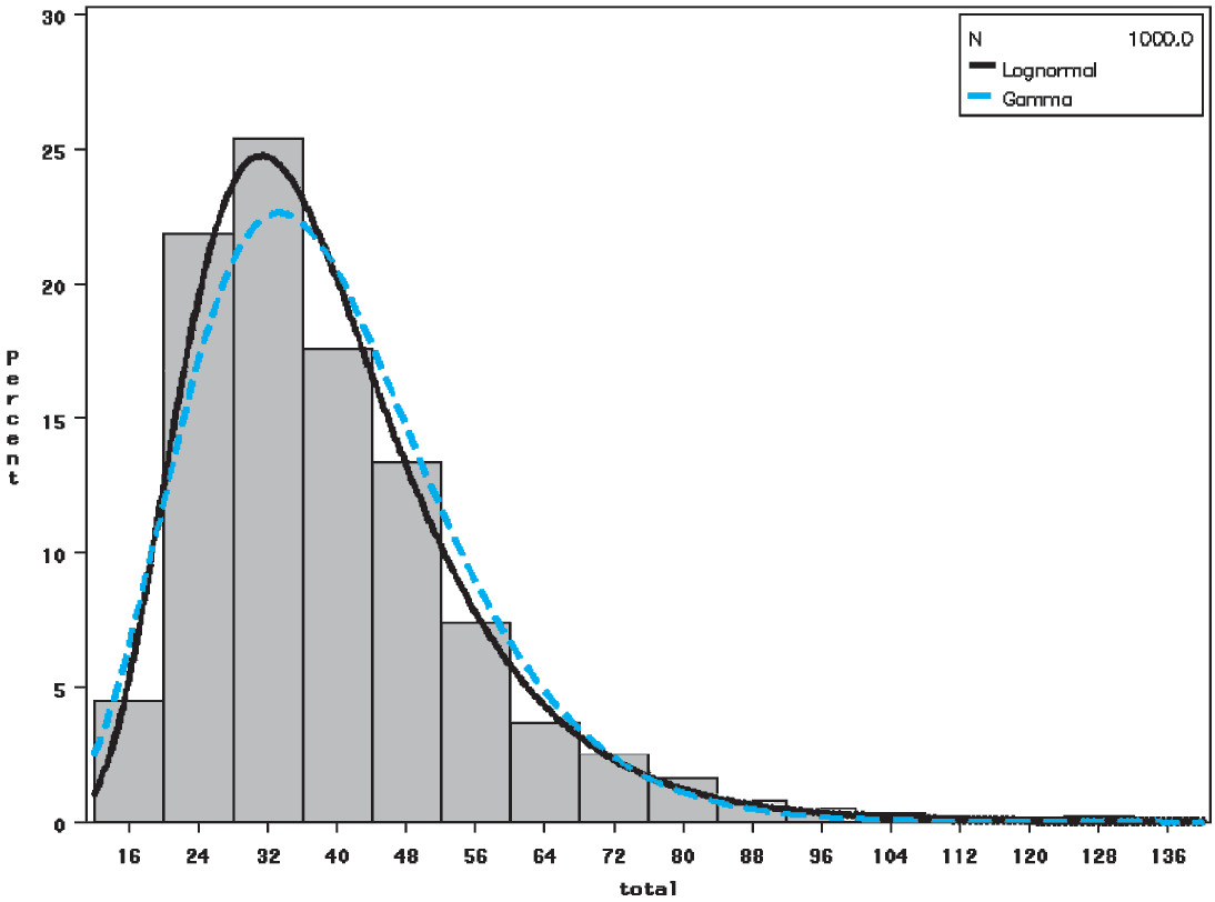
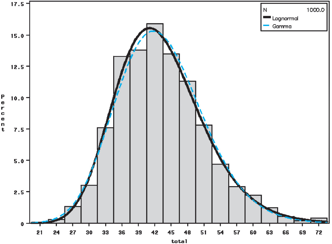
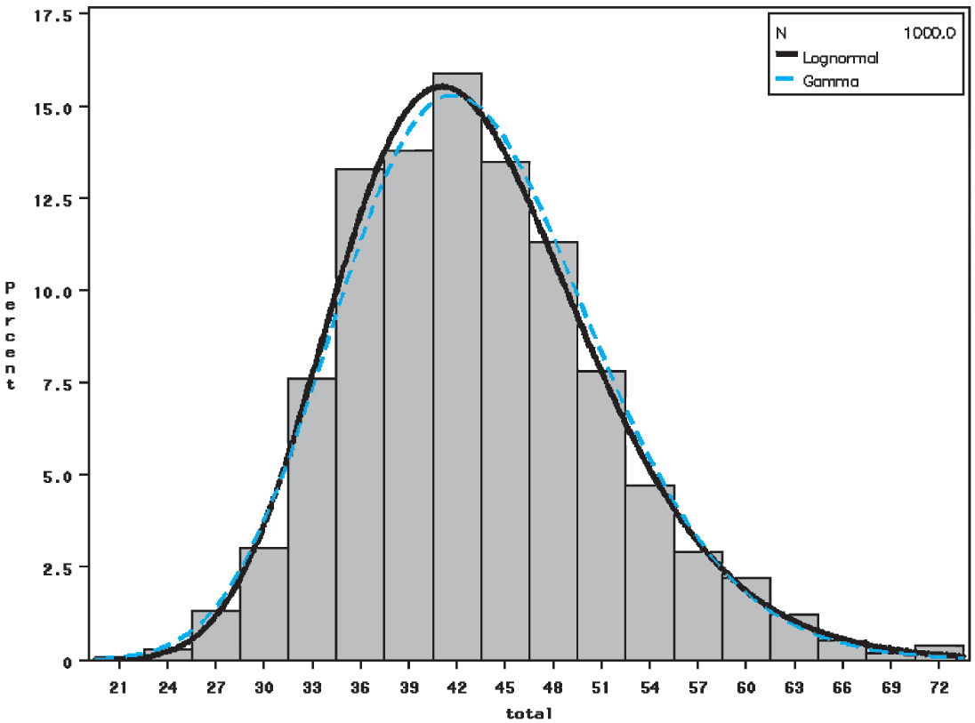
Histograms of the bootstrapped distributions for each of the models, each with 1,000 replications, are presented in Figures 6, 7, and 8. These graphs all relate to jurisdiction 0.
In the application of the blending algorithm in Section 3.5, the following decisions were made:
-
Both log and linear blending were considered; for these data the log blending was found to perform the better;
-
Only variances were used in the blending algorithm (i.e., the covariance matrix in Equation (3.50) was assumed to be strictly diagonal);
-
The progression of weights, and the ratio of blended liability to case estimates, were smoothed over accident years 1 to 13 only. For year 14, the minimum variance unbiased estimates were used since the case estimates for the most recent year are considerably lower than those in previous years, due to the immaturity of that experience (only one quarter into the accident year). Using them in the smoothing algorithm would have led to distorted results;
-
Negative weights were not allowed (see the discussion at the end of Section 3.5);
-
Values of k1 = k2 = 1014 were selected. These values were selected by first choosing values of similar order to the matrices B and T in (3.58) and then examining plots of case estimate ratios and weights for a suitably smooth progression (e.g., Figures 9 to 11).

_and_l___1_(right_graph).png)
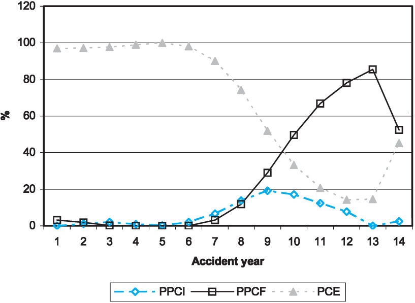
The weights that result from the algorithm are shown in Figure 9 (jurisdiction 0) and Figure 10 (jurisdiction 1). The omission of smoothing in the last year is evident from the graphs. As would be expected from the results in Table 1 and 2, the PPCI model is assigned low weights in both models.
A final point to note is the relatively high weight assigned to the PCE model for accident year 14, particularly for jurisdictional grouping 1. Although the PCE results for year 14 have a high coefficient of variation (refer to Tables 1 and 2), the quantum of liability is small relative to the other models, meaning, in turn, that the standard deviation in absolute terms is low.
The practitioner may wish to intervene to increase the standard deviation to a level perceived as realistic relative to the other models. This has not been done here, however.
The ratio of the blended liability (that results from the weights above) to case estimates is shown in Figure 11, in which the horizontal axis relates to accident years. Given the immaturity of the case estimates in year 14 (the most recent), this comparison has been omitted. It is seen that the progression is satisfactory. Missing ratios exist in Years 1 and 3 in jurisdiction 1, as case estimates are zero in these years.
The final results are given in Table 3. It is observed that the coefficients of variation are generally lower than the individual coefficients of variation from each component model, particularly for the coefficient of variation for the total liability.
6. Discussion
The practicalities of the application of the analytical GLM filter (Taylor 2008) to claims data have been described in this paper. Also discussed are appropriate methods for bootstrapping filtered data as well as algorithms for blending the results from two or more models.
The filter described here is applied on a row-by-row basis. In insurance terms, this means that accident period changes may be incorporated easily into the model, but there is no easy way to incorporate diagonal effects (e.g., calendar period effects such as superimposed inflation). Further, data naturally arise on a calendar-year basis. Therefore, an implementation of the filter by calendar period would be useful. In principle, this should be relatively straightforward [e.g., see the description of the Kalman filter by calendar period in Taylor (2000)]. However, in practice, a number of issues may need to be addressed, such as stability of parameter estimates. This is the subject of future work.
Such methodology has potential use as part of an automatic reserving process. Within the general insurance industry, many valuations take place on a “revolving door” basis, i.e., one valuation finishes only for the next one to begin. Since filters adapt to changing experience, an automated process could be set up which would apply filters, run the bootstrap and blending process, and produce final results, without human intervention. This would lead to considerable savings in the valuation process while still producing fully stochastic models.
An automatic approach would require a range of diagnostic tests to alert users to problems which require intervention. Developing such tests is the subject of current work.
The analytical GLM filter implements an approximate solution to a Bayesian updating problem, and uses bootstrapping to estimate the distribution of predicted liabilities. More exact results may be found using a method like MCMC which can generate Bayesian posterior distributions using simulation. A comparison between the filter presented here and more exact approaches, including MCMC, will be presented in a separate paper.
The models implemented here are dynamic models, rather than static models. This means that their parameters evolve through time and that the estimates of those parameters can change through time in response, should this be warranted by experience. An example of this movement is given in Figure 12, where the PPCI model fitted to the first accident year is compared with the models for a number of following accident years.
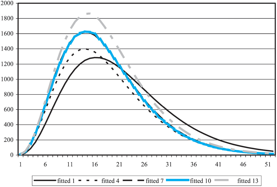
The amount of movement permitted in the fitted curves is dependent on the “parameter variances,” defined in Equation (3.19) (gamma case of the Analytical GLM filter) and Equation (3.30) (Poisson case). The choice of parameter variances may be thought of as picking a point along a continuum of levels from variances of zero (which corresponds to a static model) to high variances (each accident period modeled on just its own data, without any reference to other periods).
The selection of the variance levels is currently based on judgment; developing a more objective way to select the variances is currently being investigated.
Acknowledgments
We would like to thank Insurance Australia Group for their support of this work.