Loss Reserve Estimates

The work of science is to substitute facts for appearances and demonstrations for impressions.

—John Ruskin

1. Introduction

The work of the actuary in developing loss liability estimates is a relatively scientific process, yet by necessity it is guided by some very subjective terms like “reasonable.” The purpose of this paper is to clarify the differences in the term “reasonable reserve estimate” as it could be applied to range versus distribution estimates when evaluating management’s best estimate of reserves within that range or distribution. Along the way, the paper will show how the current broad guidelines could be “misinterpreted.” The first step in clarifying these differences is to start with a solid foundation, so this paper begins by reviewing some “codified” terms and their definitions, defining some terms for use in this paper, and reviewing various statistical measures of risk. Next, it examines some of the current practices for determining “reasonableness” and suggests a framework for defining “reasonableness” more precisely. Then various risk concepts are reviewed and (more importantly) related to the question of “reasonableness.” Once all of these definitions and concepts are outlined, some general models for calculating ranges will be examined and some practical applications will be reviewed to see how these principles might be applied in practice. Finally, the paper concludes with an overview of the findings and suggestions for further research.

2. Definition of terms

Throughout this paper, unless noted otherwise, loss reserves are intended to include both loss and allocated loss adjustment expense reserves.^[1] The Statements of Statutory Accounting Principles (SSAPs) and Actuarial Standard of Practice (ASOP) No. 36 contain some definitions related to the term “reasonable.” From the SSAPs we have the following:

Management’s Best Estimate—Management’s best estimate of its liabilities is to be recorded. This amount may or may not equal the actuary’s best estimate.

Ranges of Reserve Estimates—When management believes no estimate is better than any other within the range, management should accrue the midpoint.^[2] If a range can’t be determined, management should accrue the best estimate. Management’s range may or may not equal the actuary’s range.

Best Estimate by Line—Management should accrue its best estimate by line of business and in the aggregate. Recognized redundancies in one line of business cannot be used to offset recognized deficiencies in another line of business.^[3]

From ASOP No. 36, we have the following:

Risk Margin—An amount that recognizes uncertainty; also known as a provision for uncertainty.

Determination of Reasonable Provision—When the stated reserve amount is within the actuary’s range of reasonable reserve estimates, the actuary should issue a statement of actuarial opinion that the stated reserve amount makes a reasonable provision for the liabilities.

Range of Reasonable Reserve Estimates—The actuary may determine a range of reasonable reserve estimates that reflects the uncertainties associated with analyzing the reserves. A range of reasonable estimates is a range of estimates that could be produced by appropriate actuarial methods or alternative sets of assumptions that the actuary judges to be reasonable. The actuary may include risk margins in a range of reasonable estimates, but is not required to do so. A range of reasonable reserves, however, usually does not represent the range of all possible outcomes.

From the proposed ASOP regarding Property/Casualty Unpaid Claim and Claim Adjustment Expense Estimates (Unpaid Claim ASOP) (2006), we have the following:

Actuarial Central Estimate—An estimate that represents a mean excluding remote or speculative outcomes that, in the actuary’s professional judgment, is neither optimistic nor pessimistic. An actuarial central estimate may or may not be the result of the use of a probability distribution or a statistical analysis. This definition is intended to clarify the concept rather than assign a precise statistical measure, as commonly used actuarial methods typically do not result in a statistical mean.

These definitions provide the actuary with only broad guidance on what is “reasonable.” For example, is any reserve considered “reasonable” if it falls within any range of estimates based on any set of assumptions and methods that are deemed reasonable by a competent actuary?^[4] Of course any set of assumptions and methods deemed reasonable by the actuary must also stand up to peer review scrutiny, but does this imply that two actuaries can create a quorum for determining reasonableness? Should the actuary’s judgment about the assumptions and methods be the only criteria for reasonableness, or do we need additional context to put these questions in perspective? In essence, these terms seem to imply a “reasonable person” standard much like you would find in a legal context.

From a historical perspective, most of these definitions have roots dating back to when only deterministic methods were available to the actuary. More recent advancements, especially in the last few decades, have added a wide variety of stochastic models to the actuary’s toolkit. While the principles and standards noted above recognize that the actuary’s liability estimate could be a deterministic point estimate or derived from a stochastic distribution, they are generally silent when it comes to elaborating on the differences between these two types of estimates.

Thus, this paper will explore some of the differences between point estimates and distributions, with particular emphasis on how the differences relate to our standards and principles, and it will put forth the premise that a statistical approach should be added to the “reasonable person” standard so that risk management considerations, by both actuaries and users of the actuarial work product, related to whether a stated reserve is “reasonable” can be made. In order to develop this approach, some basic definitions are offered. Consider the following:

• Reserve—An amount carried in the liability section of a risk-bearing entity’s balance sheet for claims incurred prior to a given accounting date.

• Liability—The actual amount that is owed and will ultimately be paid by a risk-bearing entity for claims incurred prior to a given accounting date.^[5]

• Loss Liability—The expected value of all estimated future claim payments.

• Risk (from the “risk-bearer’s” point of view)—The uncertainty^[6] (deviations from expected) in both timing and amount of the future claim payment stream.^[7]

• Method—A systematic procedure for estimating future payments that does not involve the use of any statistical assumptions that could be used to validate reasonableness or to calculate standard error and that is used to estimate a deterministic point estimate of the loss liability.^[8],^[9]

• Model—A mathematical or empirical representation of how losses emerge and develop that accounts for known and inferred properties and is used to estimate a stochastic distribution of the future claim payments and from which the loss liability can be estimated.

3. Measures of risk

From statistics, actuaries often use a variety of measures that help describe risk. These measures could include variance, standard deviation, skewness, average absolute deviation, value at risk, tail value at risk, etc., which are measures of dispersion.^[10] Other measures that help to define aspects of the distribution that might be useful in determining “reasonableness” could include mean, mode, median, etc. The choice for measure of risk will also be important when considering the “reasonableness” and “materiality” of the reserves in relation to the capital position.

For insurance risks, actuaries often discuss the need to consider both “process” and “parameter” risk since both of these are part of the risk-bearer’s burden.

Process Risk—The randomness of future outcomes given a known distribution of possible outcomes.

Parameter Risk—The potential error in the estimated parameters used to describe the distribution of possible outcomes, assuming the process generating the outcomes is known.

Statistically, both of these can be measured and used to calculate the distribution of possible outcomes. However, these calculations assume that the process that is generating the outcomes is known and the only requirement is to estimate the parameters of that process. Thus, for the purpose of describing a full range of possible liability outcomes, another type of risk could be added:

Model Risk—The chance that the model (“process”) used to estimate the distribution of possible outcomes is incorrect or incomplete.^[11]

Consider an example from gambling. In the game of roulette, the casino knows exactly what the distribution of numbers and colors are on the roulette wheel, so determining the payouts (odds) involves only the process risk for the game since the parameters are certain (assuming a fair game). If we were to change the game so that the casino did not know the exact distribution of numbers and colors, then the casino could only determine appropriate payouts by continuous sampling of the outcomes.^[12] In this case the casino, like the insurance risk-bearer, does not know the exact parameters of the game, so excluding the “parameter” risk from its payout calculations could lead to potential bankruptcy or, at a minimum, less profit than was expected.

So far this example explicitly assumes that the game still resembles a game of roulette, except that the numbers on the wheel are not known in advance. If we were to change the game even more, so that the casino did not know how the outcomes are produced, then the casino would also be forced to guess at the process used to create outcomes when it is estimating the odds from its continuous sampling. The observed outcomes may resemble the outcomes from one or more mathematical distributions, which can be used to estimate the parameters, but the actual process that is generating outcomes is still unknown. Again, the casino, like the insurance risk-bearer, would need to add in an additional “risk load” in order to include “model” risk and be properly compensated.

Returning to the insurance world, if there were no risk there would be no need for insurance. Even if there were no parameter or model risk, the insurance risk-bearer would still have some chance of insolvency. Failing to recognize parameter and model risk increases the danger of insolvency. Returning to the earlier definition of loss liabilities, this analogy would imply that all three types of risk (i.e., process, parameter, and model risk) should be included as part of the calculated expected value. Alternatively, some or all of these types of risk could be included in a “risk margin” as defined under ASOP No. 36.

Before moving on to look at how these various types of risk relate to the reasonableness of reserves, note that standard statistical techniques (and terminology) are already available and, hence, do not need to be reinvented, but the nuances of the definitions may require us to be more explicit in our terminology. For example, standard deviation and standard error have slightly different formulas and different meanings. Standard deviation describes a characteristic of a known distribution and includes only “process” risk, while standard error is an estimate of that characteristic of the underlying distribution based on sample data and includes both “process” and “parameter” risk. Unfortunately, calculating model risk may not be possible.^[13] While model risk is implied with the common definition of parameter risk and, therefore, assumed to be included in standard error calculations, it would seem more prudent to include a separate measure or loading for model risk.

4. How do we define “reasonable”?

In accordance with the SSAPs and ASOPs, the actuary must opine on the reasonableness of management’s reserves, but the definition of what constitutes “reasonable” simply refers to a range. Thus, the actuary, and management, needs to consider a range of estimates, but there seems to be no defined process for determining what is “reasonable” within this range or whether the range itself is “reasonable.”^[14]

From a historical perspective, the focus on a range originated from a recognition that a method only produces a single point estimate and that any given method may be an imperfect estimation tool. Thus, the actuary’s judgment regarding the “best estimate” is better informed by using a variety of methods that produces a range of point estimates. Even though ASOP No. 36 and the Unpaid Claim ASOP hint at modeling and distributions, they remain focused on ranges. While we must recognize that some situations may always require the use of point estimates and ranges, clarifying the differences between ranges and distributions will allow us also to focus on how the “reasonableness” standard could be applied to each.

4.1. The problems with point estimates

Starting with a range of point estimates, a range, by itself, creates several problems that need to be overcome in order to determine “reasonableness”:

• A range (arbitrary or otherwise) can be misleading to other risk managers or outsiders—it can give the impression that any number in that range is equally likely.

• A range can also give a false sense of security—it gives the impression that as long as the carried reserve is “within the range” anything is reasonable (and therefore in compliance) as long as it can be justified by other means.

• There is currently no specific guidance on how to consistently determine a range within the actuarial community (e.g., ±X%, ±$X, using various estimates, etc.).^[15]

We can illustrate the first two of these problems with an example. Starting with a game of chance where you wager a certain amount ($X) and in return you receive the dollar amount for the number that turns up on a roll of a fair die plus $10, the range of possible outcomes is $11 to $16 and the expected value is $13.50, so a fair wager is $13.50. A higher wager would be “good” for the house (it would gain over time), while a lower wager would be “bad” for the house (it would lose over time). Converting this to an insurance example, suppose an actuary was to tell management that the expected value of the liability estimate is $13.5 million, but the estimated range is $11 to $16 million and that each value in that range is equally likely to occur. What values in that range are “reasonable” for management to accrue?

While the sophisticated risk manager might recognize that there is a distribution of possible outcomes behind the scenes in this example, the unfortunate truth is that the individual point estimates that form this range do not provide us with any statistical information (either individually or collectively) about the shape of the distribution. Thus a range, in and of itself, has insufficient meaning without some other context to help define it with respect to defining “reasonableness” more precisely.

4.2. The advantages of distributions

Shifting our focus to a distribution of possible outcomes, it is possible to define “reasonable” more precisely such that the reserves would be sufficient to cover all future estimated claim payments at least X% of the time.^[16] Alternatively, we could define a “reasonable” probability range based on the distribution of possible outcomes, which can be translated into a range of liabilities that correspond to those probabilities. For example, telling management the liability estimate is $13.5 ± $2.5 lacks sufficient meaning because of the reasons noted above. However, continuing the earlier example, the actuary could advise management that reserves of a least $13.5 million were required in order to achieve a 50% probability that they were sufficient and that $14.75 million would be required in order to increase the probability that they would be sufficient to 75%. This would give the range some context for “reasonability” that management could use to set reserves. In effect, the second approach will be much more meaningful to management and other users of actuarial reports.

In addition to defining which portion of the distribution would constitute the “reasonable” reserve portion, several other advantages arise when a model is used to estimate a distribution.

4.3. The probability range

Using a probability range to define a range of reasonable liabilities has the advantage of using the “risk” inherent in the data to define the range instead of a simple constant percentage (or constant amount). For example, if we were to define “reasonable” as a probability range of 50%–75%, then the corresponding range of reasonable reserves might be $97–$115 for a line of business (see Table 1) with a relatively stable claim payment stream, while the corresponding range of reasonable reserves might be $90–$150 for a line of business with a more volatile claim payment stream, even though both lines have an expected value of $100. Contrast this with the common approach of using the estimated liabilities ±X% for each line of business.

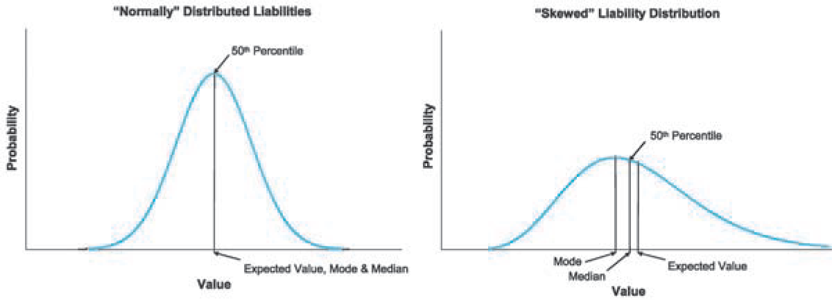
Using a probability range will also add context to other statistical measures. For example, as most liability distributions are skewed to the right, the mean will usually represent a value that is greater than the 50th percentile and can be used to help illustrate how the potential for the actual outcome to be worse than expected is greater than the potential to come in better than expected. Some actuaries have argued that the mode or the median could also be considered when describing what is “reasonable” in this context but, like the mean, discussing these as part of a probability range will complete and tie these various measures together.

4.4. The mode and median

The argument for using the mode as the “reasonable” reserve is that it has the highest probability of actually occurring. However, since liability distributions are usually skewed to the right, the mode would generally be less than the 50th percentile, as illustrated in Figure 1. In the context of liability distributions, the mode is the least desirable option for the low end of the range. Looking at the median (50th percentile), this would appear to be a logical low end to a range of “reasonable” reserves, but care must be exercised when selecting reserves by line of business compared to the aggregate reserves for all lines combined.

Figure 1.Comparison of “normal” vs. “skewed” liability distributions

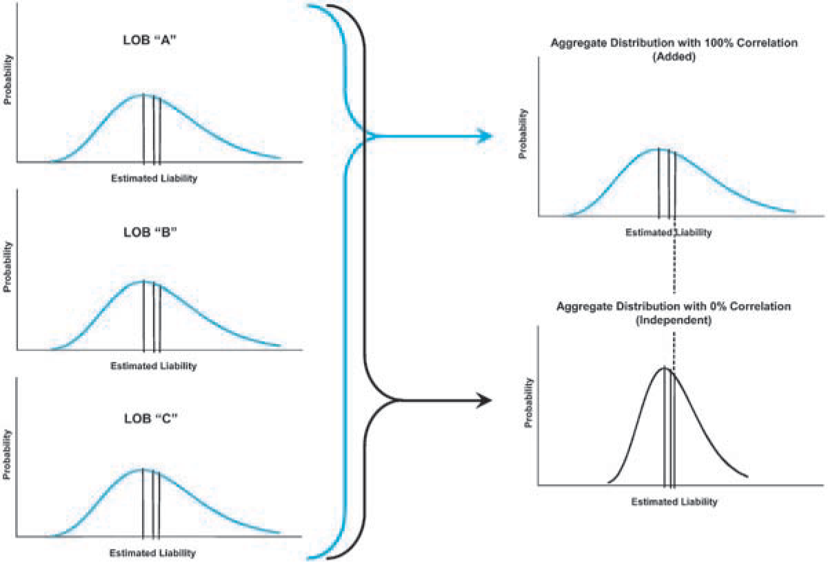
When reserves are selected by line of business and then simply added together to arrive at the total for all lines of business combined, this process is the same as assuming 100% correlation between lines. Generally, there is some level of independence between lines (i.e., less than 100% correlation), which means that the total of selected individual medians (or modes) will be less than the median (or mode) of the aggregate for all lines combined. This concept is illustrated in Figure 2. Thus, if the median (or mode) is considered to be a “reasonable” low end for a probability range, then the medians (or modes) for the individual lines of business will need to be adjusted so they sum to the median (or mode) for the aggregate of all lines.^[17] Using the expected value as the low end of the “reasonable” probability range will avoid this problem.^[18]

Figure 2.Comparison of aggregate liability distributions

4.5. The reserve margin

The concept of a “reserve margin” is often discussed in terms of a prudent excess over the expected value (or “best” estimate for deterministic methods).^[19] This definition of reserve margin is consistent with using probability ranges. For example, if the carried reserve is greater than the expected value, then the reserve margin is the difference between the carried reserve and the expected value.^[20] However, nothing in this paper should be construed as implying that a carried reserve margin is not reasonable. On the contrary, recognition of “process,” “parameter,” and “model” risk would imply that having a reserve margin is not only reasonable but prudent.

More importantly, the recognition of “process,” “parameter,” and “model” risk can often result in a higher estimate of the expected value from a stochastic model when viewed next to a point estimate from a comparable deterministic method. This calls into question the need to clarify the difference between measuring and recognizing “uncertainty” in a liability estimate versus recognizing a margin. For example, all else being equal, adding model risk to a distribution would increase the expected value and decrease the reserve margin, but should the model risk already have been included in the reserve margin estimate? In other words, a desired reserve margin based on an expected value calculated with only parameter risk (or a deterministic point estimate) should be larger, all else being equal, than a reserve margin based on an expected value that includes parameter, process, and model risk. In order to avoid confusion, clarifying the types of risk included in the calculation of expected value should be disclosed.

4.6. The relationship between reserves and surplus

At the high end of the probability range, considerations related to materiality^[21] of the reserve compared to the resulting surplus come into play. One way to tie materiality to the probability range (of liabilities) would be to use dynamic risk modeling to estimate how liability outcomes relate to the probabilities of insolvency. Consider the following possibilities shown in Table 2.^[22]

The relationship between reserve risk and the risk of insolvency is a complex issue. As illustrated in Table 2, there is a very strong interrelationship between how well an insurance enterprise is capitalized and the magnitude of the reserve risk. As a general rule, increasing the amount of the carried reserves will directly decrease the amount of surplus (Surplus = Assets − Liabilities), but the probability of insolvency wouldn’t necessarily change.^[24] As a corollary to this rule, if two companies have the same distribution of loss liabilities but Company A has only half the surplus as Company C, the probability range is the same for both companies even though the probability of insolvency for Company A is significantly higher.

Viewed over time, if Companies A and C both change their mix of business in such a manner that it increases their reserve risk (from, say, “low” to “high” risk), then the probability of insolvency will also increase for both but not to the same degree. Of course, insolvency risk also depends on several other types of risk such as pricing risk, asset default risk, interest rate risk, reinsurance risk, catastrophe risk, etc. However, when all else is equal, the probability of insolvency decreases as the amount of surplus increases and increases as the reserve risk increases.

Interestingly, statistical analysis using ruin theory shows that pricing to the expected value every year, without any margin for risk loading, will eventually lead to insolvency with probability of 100%.^[25] Since the distribution of future liabilities is a critical input for pricing, this suggests that a prudent lower bound to the “reasonable” probability range should be at least the expected value, if not higher, although higher would depend on whether or not the expected value included parameter, process, and/or model risk.

From the tables and discussion above, we might assume that a probability range from the expected value to 90% is “reasonable” so that every company can recognize the impact of reserve risk on its balance sheet and be properly compensated for risk in its pricing. Since market considerations related to “perceived” undercapitalization and the distortion of earnings that occur when a company strengthens its reserve position within this range put a natural economic barrier on the high end of the range, it seems like most regulators would be mainly concerned with keeping carried reserves above the low end of the probability range. Alternatively then, we might consider any carried reserves above the expected value to be “reasonable.”^[26]

4.7. The relationship to materiality

Relating the concept of materiality to a probability range could also prove useful in other related areas such as discussions of risk-based capital and other solvency measures. For example, in a recent paper by Herbers (2002), the viewpoints of different users of Statements of Actuarial Opinion are considered and a variety of sources for defining materiality are identified. Among all the different interests identified, the common goal among them is to make sure that risk is adequately disclosed. Conversely, the differences seem to be related to what level of risk needs to be disclosed. In order to satisfy the needs of all different users of actuarial opinions, the author suggests using the principles of greatest common interest and of least common interest, defined as follows:

Principle of Greatest Common Interest—The “largest amount” considered “reasonable” when a variety of constituents share a common goal or interest, such that all common goals or interests are met.

Principle of Least Common Interest—The “smallest amount” considered “reasonable” when a variety of constituents share a common goal or interest, such that all common goals or interests are met.

These principles could be used separately or in conjunction with each other, depending on which goal or interest is being considered. For example, at the low end of a probability range the principle of greatest common interest would imply using the highest minimum such that the requirements of all constituents are met. For materiality, the principle of least common interest would imply using the least amount of surplus change considered “reasonable” by all constituents concerned with materiality. As a point of clarification, these principles are not intended to govern considerations related to comparing different estimates, but rather to the interpretation of external requirements.

5. Other risk concepts, assumptions, and considerations

As we move from using deterministic methods to using stochastic models, our actuarial processes move from “a search for the best pattern” toward “a search for the best overall model.” In other words, using methods can be characterized as trying to find the future incremental expected value path, while using models can be characterized as trying to find all possible outcomes for the future path. Indeed, Hayne^[27] eloquently described the “Holy Grail of reserve uncertainty” as “the distribution of the amount and timing of future payments for a particular book of policies” [emphasis added]. Thus, the actuarial search for the Holy Grail is the search for the model that describes that distribution.

While qualitative measures are useful in the evaluation of deterministic methods, they are of vital importance as we search for the Holy Grail. Therefore, before discussing the practical aspects of actually calculating probability distributions, it is important to review some modeling concepts, assumptions, and considerations that will be relevant to the qualitative review of various models.^[28]

5.1. The covariance concepts

Covariance is important, both by year and line of business, as a tool for evaluating the overall quality of a model.^[29] Thus, the following seven concepts can be thought of as useful tools for evaluating the quality of a model.

• Concept 1: For each (accident, policy, or report) year, the coefficient of variation (standard error as a percentage of estimated liabilities) should be the largest for the oldest (earliest) year and will, generally, get smaller when compared to more and more recent years.

• Concept 2: For each (accident, policy, or report) year, the standard error (on a dollar basis) should be the smallest for the oldest (earliest) year and will, generally, get larger when compared to more and more recent years.^[30] To visualize this, remember that the liabilities for the oldest year represent the future payments in the tail only, while the liabilities for the most current year represent many more years of future payments including the tail. Even if payments from one year to the next are completely independent, the correlated sum of many standard errors will be larger than the correlated sum of fewer standard errors.

• Concept 3: The coefficient of variation (standard error as a percentage of estimated liabilities) should be smaller for all (accident, policy, or report) years combined than for any individual year.

• Concept 4: The standard error (on a dollar basis) should be larger for all (accident, policy, or report) years combined than for any individual year.

• Concept 5: The standard error should be smaller for all lines of business combined than the correlated sum of the individual lines of business—on both a dollar basis and as a percentage of total liabilities (i.e., coefficient of variation).

• Concept 6: In theory, it seems reasonable to allocate any overall “reserve margin” (selected by management) based on the standard error by line after adjusting for covariances between lines.

• Concept 7: Whenever simulated data is created, it should exhibit the same statistical properties as the real data. In other words, the simulated data should be statistically indistinguishable from real data.

5.2. The model assumptions

To simplify the calculations, claim payments by period are often assumed to be Normally distributed in many of the commonly used models for estimating liabilities. This can be a useful assumption for calculating a closed form solution, but the actuary must be very careful when using these assumptions with real data. Therefore, the four “assumptions” described below are tools for evaluating the quality of a model.

• Assumption 1: For lines of business with small payment sizes (e.g., Auto Physical Damage) the Normal distribution might be a reasonable simplifying assumption.^[31]

• Assumption 2: For most lines of business, the distribution of individual payments, or payments grouped by incremental period, is skewed toward larger values. Thus, it would be better to model the claim payment stream using a logNormal, Gamma, Pareto, Burr, or some other skewed distribution function that seems to fit the observed values.

• Assumption 3: Estimating the distribution of loss liabilities (in total or by accident or payment period) assuming that the claims are Normally distributed could produce misleading results for management whenever the actual claims are not Normally distributed. The relevance of this distortion compared to the cost of improving the estimates needs to be considered.

• Assumption 4: Estimating the standard error in the claim payments assuming a Normal distribution and then simulating the total loss distribution using a logNormal distribution (or some other skewed distribution) is marginally better, but it will require much greater skill and care than using an assumption based on parameters assuming a logNormal (or some other skewed distribution) and testing to see how well this fits the actual data.

5.3. The use of case reserves

Since the projection of incurred losses does not directly measure the variability of the future payment stream, its usefulness in determining liability distributions should be considered. Similar to the concepts and assumptions, the following “considerations” are useful in evaluating the quality of a model.

• Consideration 1: The “extra” information in the case reserves is generally believed to add value by giving a “better” estimate of the expected mean. The exceptions to this are well documented in the actuarial literature. However, does this “extra” information really change the estimate of the a priori expected value of the payment stream (by year), or does it give a better “credibility adjusted” estimate of the likely final outcome (by year) after the additional information comes to light and leave the a priori expected value of the payments unchanged?^[32]

• Consideration 2: Consider two identical books of business with two different insurance companies.^[33] They are identical except that one company sets up case reserves on the claims and the other does not. The estimates of the total liabilities (incurred but not reported [IBNR] versus case plus IBNR) are identical. Will the deviations of actual from the expected value of the future claim payments be any different?

• Consideration 3: Since measuring the variations in the incurred claims does not directly measure the variations in the payment stream, should risk measures based on incurred claims be used to quantify risk for management? With consistent levels of case reserves, the variations in the incurred claims might be more stable and might converge more quickly toward the actual outcome, but would this measure mask some of the true volatility? On the other hand, with case reserve strengthening or weakening, the variations in incurred claims may be less stable than for paid claims and could possibly overestimate volatility. While incurred claims can improve the quality of an estimate, and data distortions can occur with both paid and incurred data, the key question here is the definition of risk. In other words, if we accept a definition of risk based on claim payment fluctuations then the analysis of incurred claims would usually need to be adjusted in order to be consistent with that definition.

6. Models for calculating ranges

Historically, the problem of estimating a distribution for a defined group of claim payments has been solved using “collective risk theory.”^[34] Actuaries have built many sophisticated models based on this theory, but it is important to remember that each of these models makes assumptions about the processes that are driving claims and their settlement values. Some of the models make more simplifying assumptions than others, but none of them can ever completely capture all of the dynamics driving claims and their settlement values. In other words, none of them can ever completely eliminate “model risk.”

The recent Reserve Variability Working Party Report includes an excellent summary of many different methods and models, including the use of a common set of terminology and notation, and a classification scheme for modeling characteristics of the different types of models.^[35] While the technical details contained in this report are very important, for the purposes of this paper a more general approach to classifying different methods and models is more effective so that we can more easily relate to the concepts, assumptions, and considerations noted in the previous section and reflect on how they are related to these general groups and our standards of practice.

6.1. General assumptions

Before moving on to the general groups, it is useful to examine some of the key assumptions common to many methods and models. For example, consider this thought exercise. Do claim adjusters base their individual claim payments on the cumulative value of past payments for each claim? No, they base each incremental payment on the circumstances at the time.^[36] Thus, claim payments are not generally related to the cumulative payments to date, at least in regard to the actions of the claims adjusters. However, a convenient simplifying assumption is made when using methods based on link ratios that the incremental payments are directly related to the prior cumulative payments. Even though there may not be a causal relationship between cumulative payments and incremental payments, a link ratio relationship can work on average, but a bias (whereby “unusually” low cumulative values tend to under-predict the ultimate and “unusually” high cumulative values tend to over-predict the ultimate) also tends to exist when using link ratios.^[37] Every actuary recognizes this bias (either implicitly or explicitly) and quite often the Bornhuetter-Ferguson method (1972) and informed judgment are used to adjust for this bias.

In fact, Venter Venter (1998) has shown that methods based on link ratios often fail to be good predictors when you test the underlying assumptions. The chain ladder method (i.e., weighted average of all link ratios) is actually a form of regression through the origin. Venter showed that quite often a better predictor is an average plus a constant (i.e., slope not through the origin) or perhaps just a constant term.

A range of estimates using methods based on link ratios should necessarily exclude using link ratio methods when the assumptions underlying the methods aren’t strictly met—i.e., they fail tests of their predictive value as described by Venter. In other words, if you have “bad” estimates, they are “bad” estimates and shouldn’t enter into the determination of the “reasonable” range.^[38] In practice, however, using the Bornhuetter-Ferguson method for the last few years (where the link ratio methods are more likely to fail) is generally viewed as a reasonable “adjustment” in approach as one failed test does not generally invalidate the entire method. Indeed, since no one test is conclusive the actuary must weight the results of a variety of tests and judgments in order to arrive at a conclusion about the best set of methods or models. In the discussions that follow, all estimates using link ratio methods are assumed to pass these tests or suitable alternatives are assumed to have been adopted.

Models based on incremental payments get around this “limitation” of the link ratio methods and also have the advantage of more directly measuring the fluctuations in the timing and amount of the future claim payment stream. On the other hand, incremental models are less well known (or at least seem to be used in practice and discussed less often) and can be more difficult to apply for certain data sets. As always, the practicing actuary needs to be familiar with the advantages and disadvantages of each method and model used to estimate liabilities.

For purposes of this paper, the methods and models used to calculate liability ranges and distributions will be grouped into four general categories: multiple projection methods, statistics from link ratio methods, incremental models, and simulation models.

6.2. Multiple projection methods

In this category, the actuary uses multiple methods and possibly various assumptions for each method to come up with a variety of possible estimates. Usually this involves methods based on link ratios (at least in part), and it is generally assumed that these various estimates are a good proxy for the variation of the expected value of the possible outcomes. This process is limiting, with regard to distributions, in several important respects:

• The projected estimates produce a range, but it does not provide a measure of the density of the distribution for the purpose of producing a probability function—it simply produces a range of estimates for the mean, but only to the extent that the actuary varies the methods and assumptions.^[39]

• The “distribution” of (or “variations” in) the point estimates is a “distribution” of the methods and assumptions used, not a statistical distribution of the possible future claim payments.^[40]

• While methods based on link ratios are often assumed to be estimating the expected value of the liabilities, in point of fact they only produce a single point estimate and there is no statistical process for determining if this point estimate is close to the expected value of the distribution of possible outcomes or not.

• Since there are no statistical measures for these methods, any overall distribution for all lines of business combined will be based on the addition of the individual ranges by line of business with judgmental adjustments for covariance, if any.

While there are serious statistical limitations and drawbacks to using multiple projections to determine a distribution (as opposed to a range), we must recognize that producing any range is better than no range at all. Also, data limitations may prevent the use of more advanced models for estimating a distribution. Unfortunately, multiple projections don’t provide a true probability range based on statistics, so the more sophisticated models described later would normally need to be used in practice, or appropriate caveats will need to be included in the actuarial report, whenever a distribution estimate is required.

A strict interpretation of the guidelines in ASOP No. 36 would generally lead the actuary to use this approach to create a “reasonable” range. In addition, data limitations or project requirements may limit the actuary to this approach. Thus, if it is agreed that a range includes no statistical information that will allow the actuary to point to one estimate as being better than the rest, it would seem prudent for the actuarial profession to consider clarifying the definition of “reasonable” in ASOP No. 36 by adding language similar to the following:

Whenever a range of estimates is produced, and the actuary has no further means of producing a distribution of possible outcomes or is not obligated to produce a distribution, then the midpoint of the range should be used as the minimum ‘reasonable’ reserve.

This would add language to ASOP No. 36 (and the proposed Unpaid Claim ASOP) that is consistent with the definition used in the SSAPs for “Ranges of Reserve Estimates,” which requires management to accrue to the midpoint of their range. However, the profession will still need to clarify when a “best estimate” (selected using actuarial judgment from within the range) can be used as a “reasonable” reserve as the SSAP definition of “Ranges of Reserve Estimates” seems to imply that the midpoint should be used whenever a range is produced, regardless of whether a best estimate exists or not.^[41]

6.3. Statistics from link ratio methods

In this category, the models described by either Mack (1993, 1994) or Murphy (1994) and others can be used by the actuary to calculate the standard error in the payment stream using the variation in the link ratios. The actuary can use the standard error to calculate the distribution of the liabilities using the cumulative Normal distribution or use logs to get a skewed distribution, in effect converting a method into a model. These models are better than using multiple projections with regard to distributions, but they still have limitations:

• The expected value used in these models is still based on multiple methods and is subject to most of the same limitations described above for multiple projections.

• The standard error calculations in these models often assume that the distribution of the link ratios is Normally distributed and is constant by (development) period—this violates three of the evaluation criteria noted earlier: (1) link ratios are a measure of the cumulative claim payment variations, not the incremental variations (definition of risk); (2) the claim payments are usually not Normally distributed (Assumption 2); and (3) the distributions may not be constant across (development) periods (testing of assumptions).

The standard error values from these models provide a process for calculating an overall probability distribution for all lines of business combined. However, this will require making assumptions about the covariances between lines or assuming independence among lines. Further research is needed to develop additional formulas for calculating the covariances between lines of business for these models.

The use of statistics from link ratio methods is a significant improvement over ranges based on multiple projections since the variations in the underlying data are more directly modeled and used in the results. In other words, they are focused on calculating a distribution of possible outcomes given a selected estimate of the expected value. For these models, it would also seem reasonable to apply the language suggested above (regarding using the midpoint) for ASOP No. 36 (and the proposed Unpaid Claim ASOP) to the expected value portion of the calculations.

If data limitations prevent the use of models based on incremental values, then this model will need to be used. Otherwise, incremental models would normally be preferable as incremental models are generally focused on estimating the underlying distribution rather than adding distributional properties to a selected point estimate.

6.4. Incremental models

Models based on the incremental values of claims paid from one period to the next have been under development for quite some time.^[42] These models generally overcome the “limitations” of using cumulative values and have the advantage of modeling calendar year inflation (along the diagonal) using a separate parameter(s). They also generally comply with the evaluation criteria set forth in this paper, with only a few exceptions:

• Several of the models in general use assume that the distribution of incremental claims is logNormal. The actual distribution of incremental payments may or may not be logNormal, but this is a significant improvement over models that assume Normality and generally provides a good fit to the actual data. Other skewed distributions are also used, but they generally add complexity to the formulations.

• As with the other categories, when aggregating liability estimates for individual lines of business the correlations between lines will need to be considered when they are combined. Recent papers by Brehm (2002) and Kirschner, Kerley, and Isaacs (2002) are good examples of how incremental models can be correlated and combined. Research in this area is ongoing.

• An added bonus is that some of these models allow the actuary to thoroughly test the model parameters and assumptions to see if they are supported by the data. They also allow the actuary to compare various goodness-of-fit statistics to evaluate the reasonableness of different models or different model parameters.^[43] Essentially, they allow the actuary to tailor the model parameters to fit the characteristics of the data.

For the purpose of calculating a distribution of possible outcomes, incremental models are a significant improvement over models based on link ratios since they are focused on directly calculating the distribution, with the expected value being determined from the distribution itself. The main limitation to these models seems to be only when some data issues are present.^[44]

6.5. Simulation models

Because of the complex interactions between claims, reinsurance, surplus, etc., a dynamic risk model may be needed in order to more fully test the reasonableness of the distribution of liabilities. Models from all of the previous three categories can be used to create such a risk model, but in order to evaluate them we need to focus on Concept 7.

Unfortunately, simulation models based on link ratios tend to be the least useful since they quite often exhibit statistical properties not found in the real data being modeled. Whenever link ratios are shown to be worse predictors than a constant, or link ratios plus a constant, data simulated using link ratios will be distinguishable from real data. While this problem may not invalidate the conclusions from a simulation study, it will certainly reduce the reliability of the results compared to other alternatives.^[45]

This problem with “link ratio simulations” is usually overcome with models based on incremental values. It can also be overcome with ground-up simulations using separate parameters for claim frequency, severity, closure rates, etc. As with any model, the key is to make sure the model and model parameters are a close reflection of reality.^[46]

As a final comment to this section, while the use of four general categories helps to focus the discussion, we must recognize that some models don’t fit neatly into just one category or that some of the issues discussed within a category may not apply to some models in that category. For example, the bootstrap model has characteristics from each of the last three categories of models and while it uses link ratios in the simulation process other features of the modeling process allow the simulated data to look like real data.^[47]

7. Practical considerations

Up to this point, the discussion has been mainly focused on theoretical and philosophical issues related to distributions (and probability ranges defined as part of a distribution) versus ranges. Before the paper is concluded, it will also be useful to focus on some considerations of using probability ranges in practice.

7.1. Are reasonable assumptions enough?

Some actuaries may find themselves not agreeing with the conclusion that the phrase “a reasonable range” is meaningless without some other context. Their reaction may be that context is provided by the phrase, “that could be produced by appropriate actuarial models or alternative sets of assumptions that the actuary judges to be reasonable.” In other words, the sentence, “The reasonable range is from $A to $B,” must make sense in light of reasonable statements about the history of cost drivers (such as premium, exposure, and benefit changes) and about the history of loss development (such as age-to-age factors or severity trend rates).

Turning to what is “reasonable” under the definition in ASOP No. 36, it seems safe to say that “reasonableness” is determined by the actuarial culture. By talking to other actuaries, attending conferences, talking with clients, reading the newspapers, and reading some of the actuarial literature, we maintain a culture that reflects actuarial expertise. Assumptions and statements that are consistent with this culture are necessarily reasonable, even if we personally disagree with them. Assumptions and statements that would be considered misleading in the context of that culture are usually unreasonable—but one exception is statements that are well argued and supported with data, because that is how the culture is changed over time.

The author would certainly agree that culture is an appropriate context for our guidelines, but the use of probability ranges will add a new dimension to the guidelines whenever a distribution is estimated. For example, even if every actuary in the world were to agree that all of the assumptions and methods used to develop the range $A to $B are reasonable, we are still left with the question, from a solvency point of view at least, of “What makes selecting $A as the final reserve any more or less ‘reasonable’ than $B or any other number in between?”^[48] Without any further guidance do we, as a profession, have any basis for selecting one number in the range over another?

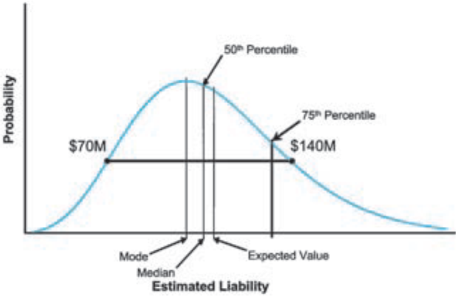
What if two or three actuaries with appropriate training and experience estimate that a given liability has a value of $100 million^[49] but the range of estimated values is $70 to $140 million based on the information, and they support their conclusion with reasonable methods and assumptions as illustrated in Figure 3? Is $70 million a reasonable estimate? Based on current standards, unless there are assumptions that are “unreasonable,” or data they have overlooked, or a mistake in their work, then the $70 million must be considered reasonable since it is “within the reasonable range” as currently described in our guidelines.

Figure 3.Which estimates in the range are “reasonable”?

On the other hand, what if those same actuaries develop a distribution of possible outcomes with an expected value of $100 million and the end points of the range noted above correspond to the 25th and 80th percentiles, respectively, as illustrated in Figure 4. If there is only a 25% chance that $70 million is sufficient to cover all future claims, then is it still a “reasonable” estimate? If the expected value of the distribution is outside of the range of point estimates, how will this impact the determination of which values in the range are “reasonable?” It is not up to the author alone to determine at what percentile an estimate changes from reasonable to unreasonable, but it sure seems like it should be much closer to the expected value (or higher) than the 25th percentile. Since no model can ever remove all of the subjectiveness from the estimation process, setting an absolute percentile that the actuary cannot go below may not be a good idea. But theoretically at least, the expected value seems to be a logical minimum for a reasonableness standard with respect to distributions.

Figure 4.Does a distribution change which estimates are “reasonable”?

A standard for distributions that is less than the expected value would be akin to recommending to a casino that it set the odds at something less than in its favor.^[50] While some constituents may consider a percentage lower than the expected value to be a reasonable lower bound, the principle of greatest common interest would suggest that other interested parties, such as stockholders, policyholders, and solvency regulators, would likely insist on at least an expected value standard as the minimum for the reasonable probability range.

Stated differently, the current guidelines seem to be saying that as long as the actuary can document the reasonableness of the methods and assumptions used to arrive at a “possible outcome” then, ipso facto, that “possible outcome” is reasonable. Rather than only reviewing the reasonableness of the underlying methods and assumptions, in and of themselves, the theory behind this paper is that the actuary also needs to look at the reasonableness of that “possible outcome” in relation to all other possible outcomes. In other words, no matter how reasonable a given method and its assumptions are, is that “possible outcome” reasonable if it is less than the expected value given a reasonable distribution of possible outcomes or, absent a reasonable distribution, given other higher estimates in the range?

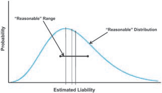
In actual practice, Figure 4 is likely to overstate the relationship between a range and a distribution. One goal of estimating a range is to come up with the “best estimate,” which could imply that the range should be as narrow as possible. On the other hand, a goal of estimating a distribution is to measure the process uncertainty, and fully reflect it in the distribution, while minimizing the parameter and model uncertainty, as illustrated in Figure 5. Ideally, then, we should recognize these differences and not confuse their purposes (and our constituents) by using imprecise terminology that implies that a range of point estimates is equivalent to a distribution of possible outcomes.

Figure 5.Distributions and ranges have different goals.

Turning to Statements of Actuarial Opinion, how should the actuary respond to the example described above if management wishes to book $70 million? Some actuaries may say, “I can’t find a way to shoot down the ‘optimistic’ assumptions that resulted in an estimate of $70 million as being unreasonable; I just think there is a lot of uncertainty.” Should the actuary then give a “clean” opinion because management made a good case but, unless something changes, include a sentence in the “risks” section of the opinion that there is a “higher than average” probability (absent a distribution or “X% probability” given a distribution) this will prove to be inadequate? Or should the actuary give a qualified opinion? This will need to be answered by the actuarial profession and other constituents that are the intended audiences for the actuarial work product. On the other hand, if management does book the expected value, at what point does the actuary need to report the high end of the liability range in the “risk” section of the opinion?^[51]

It is hoped that clarifications to the standards of practice will provide answers to these questions. In addition, the Committee on Property-Liability Financial Reporting may wish to define “risk” for purposes of a Statement of Actuarial Opinion in relation to the distribution of possible liability outcomes. For example, it could be “recommended that, if possible, the actuary disclose the 95th percentile for their estimated distribution of possible liabilities.”

Another problem with the current definition of a “reasonable range” is the way it is implemented in practice. In theory, if actuary A says that the liability is $X, and actuary B finds that this is in the reasonable range as measured by ASOP No. 9 (Documentation) (1991), ASOP No. 36 (Reserves) (2000), and the CAS principles, then actuary B should give a clean opinion. That is, actuary A, who presumably knows the situation better, is to be believed unless there is a problem. In practice, insurance companies can use the existence of the “reasonable range” as currently defined to create space to manage earnings. If “probability standards” are added, actuary A would then be required to report where he or she believes $X is with respect to the probability distribution of possible outcomes. In addition, actuary A could also be required to treat any material change in this percentage from one year to the next as a change in management procedures.^[52]

It is easy to see how well-intentioned, experienced actuaries could follow the standards of practice to the letter and end up signing a clean opinion on reserves that have a “high” probability of being deficient. In addition, in practice some of the method deficiencies described in the previous section could be compounding this issue by distorting the quality of the actuary’s calculated range.

The wording in the ASOPs was worked out by actuaries who were familiar with mathematical models and yet decided that such models did not provide the solution or were not yet sophisticated enough to provide a solution. It may be safe to surmise they were concerned that mathematical models alone do not create a wide enough “safe harbor” for actuarial practice. Yet, given the questions raised by looking at probability ranges, one has to wonder if we might have inadvertently created a “safe harbor” that is potentially too wide at the low end? While there are many references to “uncertainty” in the ASOPs, additional guidance on what should be disclosed at the high end of the range or distribution also seems appropriate.

7.2. The evolution of information

It can be said that a “reasonable” range is a function of evidence, not just possible outcomes. For example, if the only information about a block of business is that it was priced to produce an 80% loss ratio, then the only reasonable liability estimate one can make is 80% of earned premium. The range widens and shifts as, and only as, other evidence emerges showing that other outcomes are reasonable (and perhaps that 80% is no longer reasonable).^[53]

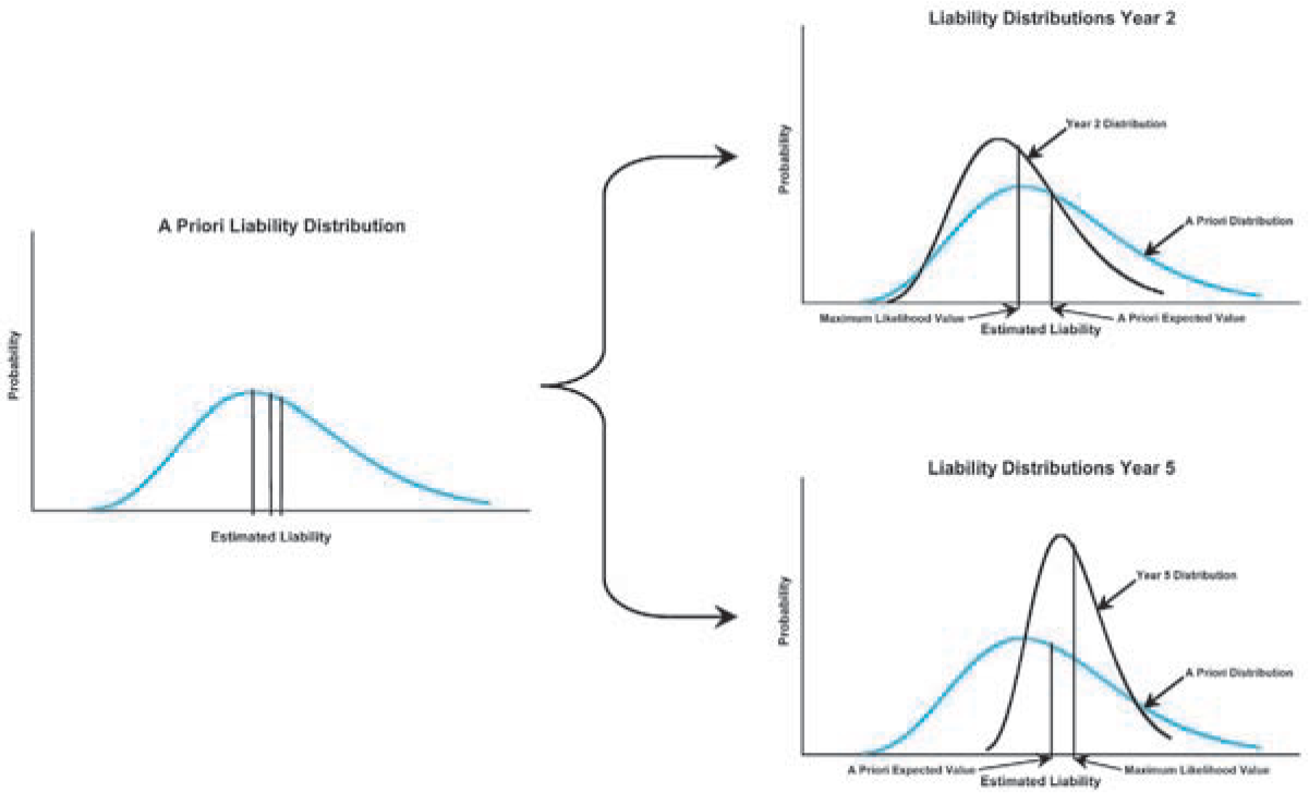
For a new block of business, the only evidence for setting reserves is the pricing documentation used to produce the rates (let’s call this “anecdotal evidence”). As this block of business is observed over time, more and more evidence (let’s call this “physical evidence”) emerges about how it is performing relative to the initial estimates and to any new updated pricing estimates (more anecdotal evidence). However, even if an 80% loss ratio is reasonable throughout this entire process, that does not mean that other outcomes are not possible at every point along the way. As time passes, the physical evidence leads us toward the actual outcome and less weight is given to the anecdotal evidence, but in general 100% weight is not given to the physical evidence until all claims are closed.^[54] While the physical evidence is leading toward the actual outcome for each year, statistically the a priori expected outcome may not be moving or may be moving in the opposite direction from the actual outcome, as illustrated in Figure 6.^[55]

Figure 6.Comparison of a priori vs. credibility adjusted liability distributions^[56]

This discussion can be summarized using one of the questions noted earlier in the paper. Namely, does this “extra” evidence really change the estimate of the a priori expected value of the payment stream (by year), or does it give a better “credibility adjusted” estimate of the likely final outcome (by year) as the additional evidence comes to light and leave the a priori expected value of the payments unchanged? While the earlier question was aimed at the merits of determining risk using paid claims versus incurred claims, it is equally relevant here.

This question, in turn, leads us to the realization that reserves are accounting fictions—they are estimates of liabilities, not the liabilities themselves.^[57] Thus, we might also look to the accounting profession for some additional principles that might be relevant. For example:

At the high end of the range, according to a general principle of accounting, a liability should not be recorded for an “event” that has not yet occurred. It is a settled issue that an “event” is the claim itself, but how far does it go to include the conditions under which the claim will be settled? For example, if inflation (as measured by the Consumer Price Index, CPI) has historically been no higher than 3% and the data for a line of business is consistent with the CPI, it seems reasonable to estimate the high end of a range assuming inflation of 3% in the future. Would the high end of the range only increase if inflation actually increased above 3%? Or is it reasonable to assume that inflation could increase above 3% and include that possibility as part of the reasonable range?^[58] Another area where these questions are relevant is with emerging theories of law or legislated changes that are allowing new claims to be filed that were not anticipated in years past. A good example here is newly emerging legal theories of asbestos liability that were not known years ago.

At the low end of the range, according to a general principle of accounting, a business should not record a profit on a particular activity until it has data to support the estimation of that profit. Accordingly, the low end of a range should be selected in order to produce zero profit in the period if there is insufficient data to establish that a profit has been earned. Recording a liability any less than $X would create the incorrect impression that the business was known to be profitable. This principle seems consistent with keeping the minimum “reasonable” reserve at the midpoint for a range or at the expected value or above for a distribution.

7.3. Who is the audience?

While it is the contention of this paper that a probability range should be used to determine what is “reasonable” whenever distributions are estimated, we must also recognize that precisely defining what a “reasonable” probability range is may depend on the audience, and, if possible, the audience should define what is “reasonable” to them. For example, solvency regulations and organizations concerned mainly about solvency (e.g., state regulators, A. M. Best’s, Standard and Poor’s [S&P], etc.) may feel that prudence would require a minimum corresponding to the expected value and a maximum of, say, 85% or 90%. Other regulatory bodies might define the “reasonable” probability range differently (e.g., the Internal Revenue Service [IRS] might consider a range from 50% to 75% to be reasonable for tax considerations and the NAIC might have different probability ranges for statutory reserves compared to rate-filing regulations). However, all of these different constituencies could use a probability range as a consistent starting point or perhaps even agree on a consistent lower bound to the probability range.

The principles of least (greatest) common interest apply when there are multiple parties that have an interest in a certain outcome. This is almost always true of actuarial reports, which means that there can be conflicting goals from the different audiences. It is easy to identify direct users of the report (management, the board of directors, regulators, etc.), but it is not always clear who might indirectly use or benefit from the report (stockholders, policyholders, consumer groups, etc.).^[59]

We should also recognize that these two principles have the potential to cause probability ranges from two different audiences to not intersect (e.g., the high end of the probability range for one party is below the low end of the probability range for another party). If this should occur, it is hoped this approach to determining “reasonableness” will provide both parties with a method for working out their differences. Alternatively, it could be used to more clearly define differences between accounting standards used for different audiences (e.g., GAAP versus Statutory versus Tax Accounting rules).^[60]

The final phrase in ASOP No. 36’s definition of the range of reasonable reserves is, “A range of reasonable reserves, however, usually does not represent the range of all possible outcomes.” While the use of a probability range is not in conflict with this statement, the example discussed in Section 7.1 shows that it is subject to interpretation. In that example, it could be used to simply state that the range from $70 million to $140 million does not include all possible outcomes. However, under a probability range approach it would be used to say, “Of course outcomes less than $100 million are possible, but they are not reasonable since the probabilities that they are insufficient are too high. On the other hand, there is a 20% chance that outcomes above $140 million are also possible and the 20% probability may be too low given model risk that is incalculable or other unforeseen events.”

Given the wide range of possible audiences for an actuarial work product, it seems prudent to err on the side of including more information rather than less. While in some cases this could increase the actuary’s exposure to malpractice, in most cases this exposure should be reduced. For example, if the unexpected happens (let’s say payments end up equaling $200 million in the example from Section 7.1. and the company ends up in bankruptcy), the actuary may be exposed to a claim of malpractice no matter what he or she said.^[61] If the actuary simply told management the range ends at $140 million, there may be some explaining to do as management may feel they were misled if they did not understand the difference between a range and a distribution. But, if the actuary provided management with a probability range and also noted that there was a 5% chance that it could reach $200 million, then management will not be able to say that this outcome was unforeseeable (and will be in a much better position to make a decision on what reserves to book).

Using a probability range, there seem to be two main reasons that actuarial malpractice could occur (excluding other potential reasons, such as fraud):

1. If the actuarial models, assumptions, or calculations used to estimate the expected value (within the distribution of possible outcomes) are faulty, or

2. If the distribution of possible outcomes is “correct” given fully tested models and assumptions, but the actuary failed to alert the proper authorities that management was booking an amount that was less than the “reasonable” minimum, whatever percentage that turns out to be.

It doesn’t seem right that getting the distribution of possible outcomes “correct,” but years later finding out that the actual outcome is higher than the expected value, would be grounds for malpractice in and of itself. However, the public perception of getting it right and actually getting it right are two different things (especially in the hands of a skilled attorney). How much longer can the actuarial profession risk telling our constituents only what is “expected” and not also telling them what is possible?

7.4. When does insolvency occur?

The previous discussions about how probability ranges are related to materiality can naturally lead to the question, “When is an insurer insolvent?” Does an insurer become insolvent when its surplus was actually inadequate or when a regulator finds out about it?

For instance, suppose a “clean” loss reserve opinion is given on the company described in Section 4 as “medium” risk in scenario A (i.e., carried reserves of $100 million, surplus of $80 million, and probability of insolvency is 60%). Years later it turns out that the paid losses for claims represented by those reserves are likely to exceed $200 million. Was the company actually insolvent when the opinion was given? Or does it become insolvent when the “higher than expected” claim payments indicate that the likely outcome will exceed $180 million? What if subsequent years improve such that cash flow never becomes an issue? What if subsequent years get worse?

At one extreme it could be reasoned that the insolvency actually took place when the clean opinion was given or even as early as when the business was written that resulted in the eventual insolvency. The rationale for this view rests on the assumption that insolvency is a technical condition, not a human discovery of that condition. This would also be distinguished from actions taken by management or regulators in response to their discoveries.

At the other extreme, it could be reasoned that insolvency doesn’t take place until the insurer reaches the point where it can’t meet current cash flow needs. Unfortunately, at this extreme the identified liabilities will usually far exceed the current assets. It’s not surprising then that regulators have set solvency requirements, via risk-based capital (RBC) requirements, so that they can take action before the insurer gets into cash flow difficulties. Therefore, a more reasonable extreme might be that the insolvency has taken place at the time the information becomes available to value the company’s surplus below RBC standards.

While both of these extremes are useful in framing the discussion, both of them rest on the assumption that future liabilities are known (or knowable with a very high degree of certainty). Until the liabilities are completely run off, no actuary can tell exactly what they will be. At either point in time (original valuation date or retroactive discovery date), two different actuaries will have two (or more) different estimates of what the liabilities are. If one estimate indicates that liabilities exceed assets and the other one doesn’t, which one is right? The answer is neither of them is right.

If liabilities are viewed as a distribution of possible outcomes, instead of an actuary’s best estimate or even a range of best estimates, at any point in time there is some probability that the future liability payments will exceed current assets (or, more accurately, future assets). So, from this perspective, the question becomes how high must this probability become in order for insolvency to occur or regulatory action to be triggered? Perhaps the added perspective of probability ranges will prove useful to actuaries and regulators as they continue to fine-tune and improve the RBC formulas.

8. Areas for future research and analysis

Throughout the paper, several areas for future research have been identified (or at least hinted at). For easy reference, they are summarized below:

• One of the theories in this paper is that measures of reserve risk should be based primarily on paid data, although some potential information from incurred data was also discussed. Research on measures of risk based on paid claims versus incurred claims would be necessary to reach any definitive conclusions. Research papers to develop models that quantify the predictive value of case reserves and credibility weight that information with estimates based on paid data would also be a valuable addition to our literature.

• Various categories of models for calculating distributions are discussed in the paper along with advantages and disadvantages of each. A research project involving retrospective testing of various models used to calculate distributions would yield insights into how significant these advantages and disadvantage are. To accomplish this, the author suggests a “blind” test with old data from multiple companies and multiple lines of business. The data should be at least 10 years old so that the final results are already known, but the tests should be run using only the triangles that would have been known 10 (or more) years ago. Alternatively, the CAS Loss Simulation Model Working Party is currently working on a model for simulating insurance data that could be used for such a purpose.

• Covariance calculation methods are a significant feature of any model used to calculate distributions for an entire company. Continuing research would always be welcome for any of the models discussed.

• Further research on the relationship between reserve risk and insolvency risk could lead to additional insights on how to define a “reasonable” probability range. It might also lead to some RBC insights or triggers for when a company should consider increasing its capitalization or when it has “enough” capital for paying dividends.

• Research on the differences between measures of reserve risk based on quarterly data versus annual data should be performed in order to help guide actuaries when dealing with issues related to quarterly versus annual accounting statements.

• The estimation of both ranges and distributions assumes a reasonable amount and quality of historical data. Research on the impact of less than ideal historical data on the ability to estimate ranges and distributions would be useful for clarifying data quality issues in our standards.

• One of the practical considerations described in the paper is about how the emergence of information might change the a priori expected value over time. How this will impact the results in practice (e.g., by using the prior point estimate as the new Bornhuetter-Ferguson expected value) could be the subject of an interesting research paper.

• The focus of this paper is the interpretation of a single actuarial analysis. However, an interesting topic for further research would be issues related to the reconciliation of two or more independent actuarial analyses. Of particular interest would be reasonable differences of opinion versus differences that could potentially lead to malpractice, and how a difference in timing of the analyses (e.g., one analysis many years after the other analysis) should be considered.

9. Conclusions

This paper started by reviewing some of the professional standards for determining the “reasonableness” of loss reserves and proceeded to examine how various statistical concepts might be used to clarify the current standards with respect to ranges versus distributions. The main conclusions of this analysis are that using a probability range has the following benefits:

• Users of actuarial liability estimates based on probability ranges will get much more information for enterprise risk management and decision making,

• The width of the dollar “range” will be directly related to the potential volatility (uncertainty) of the actual data,

• The concept of materiality can be more directly related to the uncertainty of the estimates,

• Risk-based capital calculations could be related to the probability “level” of the reserves,

• Both ends of the “reasonable” probability range will be related to the probability distribution of possible outcomes in addition to the “reasonableness” of the underlying assumptions,

• The concept of a “prudent reserve margin” could be related to a portion of the probability range and will then be directly related to the uncertainty of the estimates, and

• The users of actuarial liability estimates would have the opportunity to give more specific input on what they consider “reasonable.”

In order to implement the advantages of the statistical approach, the actuarial profession should consider adding wording similar to the following to ASOP No. 36 and the proposed Unpaid Claim ASOP:

Whenever the actuary can produce a distribution of possible outcomes, the lower bound for the reasonable range within that distribution should not be less than the expected value of that distribution.

Essentially, this paper is not proposing that we eliminate the “what a reasonable person might do” standard and replace it with probabilities. What it is suggesting is that we can improve the “reasonable person” concept by adding some additional context. There must be no illusions here. Adding a probability measure to the “reasonable person” standard will not provide a magic solution to define the exact number where the minimum “reasonable” reserves should be. Calculating the mean of the distribution is no less difficult. However, adding “probability standards” can make the “reasonable person” standards more meaningful.

In addition, the ASOP definitions of Expected Value could be improved by adding wording similar to the following:

The expected value from a distribution should include a statistically calculated amount to reflect both ‘process’ and ‘parameter’ risk and it could also include a judgmental amount to reflect ‘model’ risk. ^[62]

The word “should” in the Expected Value definition is an important consideration as it explicitly recognizes the need for the quantification of risk in the analysis. Switching the word to “could” will allow for more flexibility, but it would also increase the need for explicit disclosures and the need for more guidance on when it is appropriate to exclude “process” or “parameter” risk. As a related issue, the ASOP definitions of Risk Margin^[63] could be improved by adding wording similar to the following:

The actuary can recommend adding a risk margin to judgmentally reflect ‘model’ risk if not already included with the expected value. Alternatively, the actuary can recommend selecting a percentile above the expected value in order to create a risk margin.

Other issues mentioned in the paper that should also be addressed in our standards include (1) the need to consider language to more directly require testing of the assumptions for different models, (2) a more definitive solution for how to consistently disclose the relative reserve risk, and (3) a more precise definition of “material change” as it relates to reserve risk.

Finally, we must not forget that calculating a distribution of possible outcomes is not always possible. In that event, adding wording similar to the following to the ASOPs, as suggested earlier in the paper, would be consistent with the SSAPs:

Whenever a range of estimates is produced, and the actuary has no further means of producing a reasonable distribution of possible outcomes or is not obligated to produce a distribution, then the midpoint of the range should be used as the minimum ‘reasonable’ reserve.

In closing, ask yourself the following question: “WHAT IF you knew the EXACT distribution of possible outcomes, would you feel comfortable giving a clean opinion to a company that wanted to carry less than the expected value on their books?” As a profession we want the outside world to rely on our “actuarial judgment” to determine what is “reasonable.” Will your answer give the public added confidence in the profession? Doesn’t it make sense to strengthen our standards in order to increase public confidence?

Acknowledgments

The author gratefully acknowledges the many thoughtful comments from Oakley E. (Lee) Van Slyke on early drafts of the paper, many of which formed the basis for the section on Practical Applications. Other individuals who provided valuable contributions that improved the quality of the paper include Glen Barnett, Robert Shapland, Dean Westpfahl, Claus Metzner, Kevin Madigan, and some members of the CAS Committee on Reserves and the CAS Committee on Review of Papers. The opinions and conclusions expressed, as well as any errors or omissions that remain, are solely the responsibility of the author.

Selected Bibliography

Berquist, James R., and Richard E. Sherman, “Loss Reserve Adequacy Testing: A Comprehensive, Systematic Approach,” Proceedings of the Casualty Actuarial Society 64, 1977, pp. 123–184.

Butsic, Robert P., “Determining the Proper Interest Rate for Loss Reserve Discounting: An Economic Approach,” 1988 CAS Discussion Paper Program, pp. 147–188.

Christofides, S., “Regression Models Based on Log-Incremental Payments,” Claims Reserving Manual, Institute of Actuaries, London, 1990.

Halliwell, Leigh, “Loss Prediction by Generalized Least Squares,” Proceedings of the Casualty Actuarial Society 83, 1996, pp. 436–489.

Mack, Thomas, and Gary Venter, “A Comparison of Stochastic Models That Reproduce Chain-Ladder Reserve Estimates,” Insurance: Mathematics and Economics 26:1, 2000, pp. 101–107.

Mango, Donald, “Risk Load and the Default Rate of Surplus,” CAS Discussion Paper Program, May 1999, pp. 175–222.

Philbrick, Stephen, “Accounting for Risk Margins,” Casualty Actuarial Society Forum 1, Spring 1994, pp. 1–87.

Sherman, Richard E., “Extrapolating, Smoothing, and Interpolating Development Factors,” Proceedings of the Casualty Actuarial Society 71, 1984, pp. 122–155.

Van Slyke, Oakley E., “Regulatory Standards for Reserves,” CAS Discussion Paper Program, May 1987, pp. 368–421.

Weber, Robert A., Oakley E. Van Slyke, and Guiseppe Russo, “Loss Reserve Testing: Beyond Popular Methods,” Casualty Actuarial Society Forum, Summer 1997, pp. 381–448.

Wright, Thomas S., “Probability Distribution of Outstanding Liability from Individual Payments Data,” Claims Reserving Manual 2, London: Institute of Actuaries, 1997, Section D7.