Models of Insurance Claim Counts with Time Dependence Based on Generalization of Poisson and Negative Binomial Distributions

undefined

1. Introduction

Modeling the number of claims is an essential part of insurance pricing. Count regression analysis allows identification of risk factors and prediction of the expected frequency given the characteristics of the policyholders. A usual way to calculate the premium is to obtain the conditional expectation of the number of claims given the risk characteristics and to combine it with the expected claim amount. Some insurers may also consider experience rating when setting the premiums, so that the number of claims reported in the past can be used to improve the estimation of the conditional expectation of the number of claims for the following year.

The literature on count regression analysis has grown considerably in the past years. Simultaneously, insurers have accumulated longitudinal information on their policyholders. In this paper we want to address panel count data models in the context of insurance, so that we can see the advantages of using the information on each policyholder over time for modeling the number of claims. The existing literature has mainly advocated the use of the classical Poisson regression approach, but little has been said on other model alternatives and on model selection. Although in the insurance context the main interest is to obtain the conditional expectation of the number of claims, we argue that new panel data models presented here, which allow for time dependence between observations, are closer to the data-generating process that one can find in practice. Moreover, closed-form expressions for future premiums given the past observations and model selection will definitely help practitioners to find suitable alternatives for modeling insurance portfolios that have accumulated some years of history.

These panel data models generalize the Poisson and the negative binomial distributions into six different distributions, based on Bayesian and frequentist modeling. Some of those models are here introduced to actuarial science for the first time. Each section presents a different model for panel data, where the interpretation of the model, the probability distribution, the properties of the model, and its first moments are shown. In some sections, it is shown why some intuitive models (past experience as regressors, multivariate distributions, or copula models) involving time dependence cannot be used to model the number of reported claims. Statistical tests to compare the nested models are explained and a Vuong test is used to compare the fitting of non-nested models. Our results show that the random effects models have a better fit than the alternative models presented here. They also have more flexibility in computing next year’s premium, so that it is not only based on autocorrelation but on Bayesian modeling.

1.1. Agenda

Section 2 presents the Poisson and the negative binomial distributions in time independence situation. In Section 3, a Bayesian model for time dependence, where the Poisson and negative binomial distributions are modeled by common random effects, is shown. Models where past experience is modeled as covariate are explained in Section 4. Section 5 reviews the INAR(1) models, while Section 6 presents common shock models. Reported claims modeled by copulas are introduced in Section 7. Section 8 compares a priori premiums and predictive distribution of all models analyzed, while Section 9 presents some specification tests that can be used to compare models.

1.2. Data used and estimation

In this paper, we worked with a sample of the automobile portfolio of a major company operating in Spain. Only private-use cars have been considered in this sample. The panel data contains information from 1991 to 1998. Our sample contains 15,179 policyholders who stay in the company for seven complete periods, resulting in 106,253 insurance contracts.

We have five exogeneous variables, described in Table 1, that are kept in the panel, plus the yearly number of accidents. For every policy we have the initial information at the beginning of the period and the total number of claims at fault that took place within this yearly period. The average claim frequency is 6.8412%.

In this paper, these exogenous variables are used to model the parameters of the distributions. The characteristics of the insureds are expressed through functions such as \(h\left(\beta_0+x_{i, t}^{\prime} \beta\right)\), where \(\beta_0\) is the intercept and \(\beta^{\prime}=\left(\beta_1, \ldots, \beta_p\right)\) is a vector of regression parameters for explanatory variables \(x_{i, t}=\left(x_{i, t, 1}, \ldots, x_{i, t, p}\right)\). Subscript \(t\) may be removed where the covariates do not change over time.

Estimations of the parameters are done by maximum likelihood. Some models can be evaluated using Newton-Raphson algorithms, but we use the NLMIXED procedure in SAS to find the estimates and their corresponding standard error numerically.

2. Minimum bias and classical statistical distributions

2.1. Minimum bias

Historically, the minimum bias technique introduced by Bailey and Simon (1960) and Bailey (1963) were used to find the parameters of some classification rating systems. In these techniques, Bailey (1963) proposed to find parameters that minimize the bias of the premium by iterative algorithms. With the development of the generalized linear models (GLMs) (McCullagh and Nelder 1989), actuaries now use statistical distributions to estimate the parameters of a rating system. It has been shown that the results obtained from this theory are very close to the ones obtained by the minimum bias technique [see Brown (1988), Mildenhall (1999), or Holler, Sommer, and Trahair (1999), from the 9th exam of the Casualty Actuarial Society, that expose the link between the GLM and the minimum bias technique].

2.2. Poisson

From a statistical point of view, the common starting point for the modeling of the number of reported claims \(N_{i,t}\) for insured i at time t is the Poisson distribution:

\[ \operatorname{Pr}\left[N_{i, t}=n_{i, t}\right]=\frac{\lambda_{i, t}^{n_{i, t}} e^{-\lambda_{i, t}}}{n_{i, t}!}, \tag{2.1} \]

where \(\lambda_{i, t}=\exp \left(x_{i, t}^{\prime} \beta\right)\). Because the Poisson distribution is a member of the exponential family, from which the GLM theory comes, it has some useful properties. For more information about the technical part of the Poisson distribution for actuarial science, or even the GLM theory, we refer the interested reader to Feldblum and Brosius (2002).

However, it is well known that the Poisson distribution has some severe drawbacks, such as its equidispersion property, that limit its use (Gourieroux 1999). To correct these disadvantages, the negative binomial distributions are common alternatives.

2.3. Negative binomial

There are many ways to construct the negative binomial distribution, but the more intuitive one consists of the introduction of a random heterogeneity term θ of mean 1 and variance α in the mean parameter of the Poisson distribution. If the variable θ is following a gamma distribution, having the following density distribution

\[ f(\theta)=\frac{(1 / \alpha)^{1 / \alpha}}{\Gamma(1 / \alpha)} \theta^{1 / \alpha-1} \exp (-\theta / \alpha), \tag{2.2} \]

it is well known that this mixed model will result in a negative binomial distribution (NB) (see Greenwood and Yule 1920 or Lawless 1987 and Dionne and Vanasse 1989 for an application with insurance data):

\[ \begin{aligned} \operatorname{Pr}\left[N_{i, t}\right. & \left.=n_{i, t}\right] \\ = & \frac{\Gamma\left(n_{i, t}+\alpha^{-1}\right)}{\Gamma\left(n_{i, t}+1\right) \Gamma\left(\alpha^{-1}\right)}\left(\frac{\lambda_{i, t}}{\alpha^{-1}+\lambda_{i, t}}\right)^{n_{i, t}} \\ & \times\left(\frac{\alpha^{-1}}{\alpha^{-1}+\lambda_{i, t}}\right)^{\alpha^{-1}}, \end{aligned} \tag{2.3} \]

where the \(\lambda_{i, t}=\exp \left(x_{i, t}^{\prime} \beta\right)\) and the function \(\Gamma\) is the gamma function, defined by \(\Gamma(a)=\int_0^{\infty} e^{-t} t^{a-1} d t\). To ensure that the heterogeneity mean is equal to 1 , both parameters of the gamma distribution are chosen to be equal to \(1 / \alpha\). From this, it can easily be proved that \(E\left[N_{i, t}\right]=\lambda_{i, t}\) and \(\operatorname{Var}\left[N_{i, t}\right]= \lambda_{i, t}+\alpha \lambda_{i, t}^2\).

Cameron and Trivedi (1986) considered a more general class of negative binomial distributions having the same mean, but a variance of the form \(\lambda_{i, t}+\alpha \lambda_{i, t}^p\). This kind of distribution can be generated with a heterogeneity factor following a gamma distribution with both parameters equal to \(\lambda_{i, t}^{2-p} / \alpha\). A model with \(p=2\) is called NB2 distribution and is the previous one. When \(p\) is set to 1, it leads to the NB1 model:

\[ \begin{aligned} \operatorname{Pr}\left[N_{i, t}\right. & \left.=n_{i, t}\right] \\ = & \frac{\Gamma\left(n_{i, t}+\alpha^{-1} \lambda_{i, t}\right)}{\Gamma\left(n_{i, t}+1\right) \Gamma\left(\alpha^{-1} \lambda_{i, t}\right)}(1+\alpha)^{-\lambda_{i, t} / \alpha} \\ & \times\left(1+\alpha^{-1}\right)^{-n_{i, t}}. \end{aligned} \tag{2.4} \]

This model is interesting because its variance is equal to \(\lambda_{i, t}+\alpha \lambda_{i, t}=\phi \lambda_{i, t}\), the same used in the Poisson GLM approach (such as the one used for the overdispersion correction of the Poisson distribution in the GENMOD procedure of SAS). We can note that the Poisson distribution is the limiting case of negative binomial distributions when the parameter \(\alpha\) goes to zero.

There are many possible distributions that can be used to model the heterogeneity, such as the inverse Gaussian heterogeneity (Holla 1966 or Willmot 1987; Dean, Lawless, and Willmot 1989; and Tremblay 1992 for an application with insurance data) that leads to a closed-form distribution. Another important heterogeneity distribution is the lognormal distribution (Hinde 1982), but closed-form representation is impossible and numerical computations are needed (see Boucher, Denuit, and Guillén 2007 for an application of all these models in insurance). Other Poisson mixture models are possible (see chapter 8 of Johnson, Kotz, and Kemp 1992), but numerical techniques are also needed.

2.4. Numerical application

Results of the application of these time-independent models are shown in Table 2. A comparison of the log-likelihoods reveals that the extra parameter of the negative binomial distributions improves the fit compared to the Poisson distribution. The NLMIXED estimations of the β parameters (the intercept and the five covariates from Table 1) are approximately the same for all models, which is expected when the sufficient conditions for consistency are satisfied (see Gourieroux, Monfort, and Trognon 1984a and Gourieroux, Monfort, and Trognon 1984b).

3. Random effects

3.1. Overview

One of the most popular ways to account for a dependence that can exist between all the contracts of the same insured is the use of a common term (Hausman, Hall, and Griliches 1984). Insurance data exhibits some variability that may be caused by the lack of some important classification variables (swiftness of reflexes, aggressiveness behind the wheel, consumption of drugs, etc.). These hidden features are usually captured by the individual specific random heterogeneity term.

Given the insured-specific heterogeneity term \(\theta_i\), the annual claim numbers \(N_{i, 1}, N_{i, 2}, \ldots, N_{i, T}\) are independent. The joint probability function of \(N_{i, 1}, \ldots, N_{i, T}\) is thus given by

\[ \begin{aligned} \operatorname{Pr} & {\left[N_{i, 1}=n_{i, 1}, \ldots, N_{i, T}=n_{i, T}\right] } \\ & =\int_{0}^{\infty} \operatorname{Pr}\left[N_{i, 1}=n_{i, 1}, \ldots, N_{i, T}=n_{i, T} \mid \theta_{i}\right] g\left(\theta_{i}\right) d \theta_{i} \\ & =\int_{0}^{\infty}\left(\prod_{t=1}^{T} \operatorname{Pr}\left[N_{i, t}=n_{i, t} \mid \theta_{i}\right]\right) g\left(\theta_{i}\right) d \theta_{i}. \end{aligned} \tag{3.1} \]

Depending on the choices of the conditional distribution, of the \(N_{i, t}\) and the distribution of \(\theta_i\), the model can exhibit particular properties, as seen below.

3.2. Endogeneous regressors and fixed effects

In linear regression, correlation between the regressor and the error term leads to inconsistency of the estimated parameters [see Mundlak (1978) or Hsiao (2003) for a review in case of longitundinal data]. The same problem exists for the count data regression when \(E\left[\theta \mid x_i\right] \neq E[\theta]\) (Mullahy 1997) and it leads to biased estimates of parameters. In insurance, correlation between regressors and error term is often present (Boucher and Denuit 2005) and may be caused by omitted variables that are correlated with the included ones.

As noted in Winkelmann (2003), consistent estimates may be found if corrections are made to the standard estimation procedures. However, for insurance application, as shown by Boucher and Denuit (2005), standard methods of estimation, such as classic maximum likelihood on joint distribution based on random effects, can still be used. Indeed, the resulting estimate of parameters, while being biased, represents the apparent effect on the frequency of claim, which is the interest when the correlated omitted variables cannot be used in classification.

3.3. Poisson distribution

The simplest random effects model for count data is the Poisson distribution with an individual heterogeneity term that follows a specified distribution. Formally, we can express the classic Poisson random effects model as

\[ \begin{array}{l} N_{i, t} \mid \theta_{i} \sim \operatorname{Poisson}\left(\theta_{i} \lambda_{i, t}\right) \\ i=1, \ldots, N \quad t=1, \ldots, T, \end{array} \]

where i represents an insured and t his covering period. As for the heterogeneous models of the cross-section data model seen at the beginning of this paper, many possible distributions for the random effects can be chosen. The use of a gamma distribution can be used to express the joint distribution in a closed form. Indeed, the joint distribution of the number of claims, when the random effects follow a gamma distribution of mean 1 and variance α, is equal to (Hausman, Hall, and Griliches 1984):

\[ \begin{aligned} \operatorname{Pr}\left[N_{i, 1}\right. & \left.=n_{i, 1}, \ldots, N_{i, T}=n_{i, T}\right] \\ = & {\left[\prod_{t=1}^{T} \frac{\left(\lambda_{i, t}\right)^{n_{i, t}}}{n_{i, t}!}\right] \frac{\Gamma\left(\sum_{t=1}^{T} n_{i, t}+1 / \alpha\right)}{\Gamma(1 / \alpha)} } \\ & \times\left(\frac{1 / \alpha}{\sum_{t=1}^{T} \lambda_{i, t}+1 / \alpha}\right)^{1 / \alpha} \\ & \times\left(\sum_{t=1}^{T} \lambda_{i, t}+1 / \alpha\right)^{-\sum_{t=1}^{T} n_{i, t}} . \end{aligned} \tag{3.2} \]

This distribution, which has been often applied (see chapter 36 of Johnson, Kotz, and Balakrishnan (1996) for an overview), is known as a multivariate negative binomial or negative multinomial. Note that this distribution can also be seen as the generalization of the bivariate negative binomial of Marshall and Olkin (1990). For this distribution, \(E\left[N_{i, t}\right]=\lambda_{i, t}\) and \(\operatorname{Var}\left[N_{i, t}\right]= \lambda_{i, t}+\alpha \lambda_{i, t}^2\), so overdispersion can be accounted for. Maximum likelihood estimates of the parameters and variance estimates for them are straightforward.

The generalization of the variance of the multivariate negative binomial to obtain a form \(\phi \lambda_{i, t}\), such as the one obtained in the NB1 distribution, cannot be done directly. Indeed, since the heterogeneity term needs to be individually specific and time-invariant, introduction of covariates in the heterogeneity distribution cannot be allowed. Approximation of the covariates \(x_{i, t}\) by \(\hat{x}_i\) can be an interesting solution but cannot be used directly for prediction because characteristics of the risk at time \(t+j\) are not known for \(j>0\).

Instead, a pseudo-multinomial NB1 model can be used with the time-invariant characteristics, like the sex of the insured, and can be modeled as \(\gamma_i=\exp \left(y_i^{\prime} \delta\right)\), where \(y_i\) is a subset of the \(x_{i, t}\) that contains only these invariant covariates. Then, if we suppose that the heterogeneity is following a gamma distribution with both parameters equal to \(\gamma_i^{1-k} / \alpha\), the joint distribution can be expressed as

\[ \begin{aligned} \operatorname{Pr}\left[N_{i, 1}\right. & \left.=n_{i, 1}, \ldots, N_{i, T}=n_{i, T}\right] \\ = & {\left[\prod_{t=1}^{T} \frac{\left(\lambda_{i, t}\right)^{n_{i, t}}}{n_{i, t}!} \frac{\Gamma\left(\sum_{t=1}^{T} n_{i, t}+\gamma_{i}^{1-k} / \alpha\right)}{\Gamma\left(\gamma_{i}^{1-k} / \alpha\right)}\right.} \\ & \times\left(\frac{\gamma_{i}^{1-k} / \alpha}{\sum_{t=1}^{T} \lambda_{i, t}+\gamma_{i}^{1-k} / \alpha}\right)^{\gamma_{i}^{1-k} / \alpha} \\ & \times\left(\sum_{t=1}^{T} \lambda_{i, t}+\gamma_{i}^{1-k} / \alpha\right)^{-\sum_{t=1}^{T} n_{i, t}} ; \end{aligned} \tag{3.3} \]

where k = 1, this is the standard negative multinomial distribution (MVNB), and where k = 0 is the pseudo-multinomial NB1 equivalence (PMVNB1). Expressed in its general form, the Poisson-gamma distribution has the following moments:

\[ \begin{aligned} E\left[N_{i, t}\right] & =E\left[E\left[N_{i, t} \mid \theta_{i}\right]\right] \\ & =\lambda_{i, t} E\left[\theta_{i}\right] \\ & =\lambda_{i, t}, \end{aligned} \tag{3.4} \]

\[ \begin{aligned} \operatorname{Var}\left[N_{i, t}\right]= & E\left[\operatorname{Var}\left[N_{i, t} \mid \theta_{i}\right]\right] \\ & +\operatorname{Var}\left[E\left[N_{i, t} \mid \theta_{i}\right]\right] \\ = & \lambda_{i, t}+\lambda_{i, t}^{2} \operatorname{Var}\left[\theta_{i}\right] \\ = & \lambda_{i, t}+\alpha\left(\lambda_{i, t}^{2} \gamma_{i}^{k-1}\right), \end{aligned} \tag{3.5} \]

\[ \begin{aligned} \operatorname{Cov}\left[N_{i, t}, N_{i, t+j}\right]= & \operatorname{Cov}\left[E\left[N_{i, t} \mid \theta_{i}\right], E\left[N_{i, t+j} \mid \theta_{i}\right]\right] \\ & +E\left[\operatorname{Cov}\left[N_{i, t}, N_{i, t+j} \mid \theta_{i}\right]\right] \\ = & \operatorname{Cov}\left[\lambda_{i, t} \theta_{i}, \lambda_{i, t+j} \theta_{i}\right]+0 \\ = & \lambda_{i, t} \lambda_{i, t+j} \alpha \gamma_{i}^{k-1}, \quad j>0 . \end{aligned} \tag{3.6} \]

As for the cross-section data, other distributions can be chosen to model the random effects, such as the inverse Gaussian or the lognormal distributions [see Boucher and Denuit (2005) for an application in insurance], which result in distributions having the same two first moments as the MVNB, distinctions found using higher moments. All these random effects models come back to the Poisson distribution in the case where α → 0.

3.4. Negative binomial

The negative binomial distribution can also be used with random effects, as shown by Hausman, Hall, and Griliches (1984). Conditionally on the random effects \(\delta_i\),, the authors used a NB1 identical to Equation (2.4) except for a couple of parameter changes:

\[ \begin{aligned} \operatorname{Pr}\left[N_{i, t}\right. & \left.=n_{i, t} \mid \delta_{i}\right] \\ & =\frac{\Gamma\left(n_{i, t}+\lambda_{i, t}\right)}{\Gamma\left(\lambda_{i, t}\right) \Gamma\left(n_{i, t}+1\right)}\left(\frac{\delta_{i}}{1+\delta_{i}}\right)^{\lambda_{i, t}}\left(\frac{1}{1+\delta_{i}}\right)^{n_{i, t}}, \end{aligned} \tag{3.7} \]

where \(\lambda_{i, t}=\exp \left(x_{i, t}^{\prime} \beta\right)\). Under this parameterization, the conditional distribution has the following moments:

\[ E\left[N_{i, t} \mid \delta_{i}\right]=\lambda_{i, t} / \delta_{i}, \tag{3.8} \]

\[ \begin{aligned} \operatorname{Var}\left[N_{i, t} \mid \delta_{i}\right] & =\lambda_{i, t}\left(1+\delta_{i}\right) / \delta_{i}^{2} \\ & =E\left[N_{i, t} \mid \delta_{i}\right]\left(1+\delta_{i}\right) / \delta_{i}. \end{aligned} \tag{3.9} \]

Thus, this conditional distribution implies overdispersion. Under the construction of (3.1), Hausman, Hall, and Griliches (1984) assumed that the expression \(\delta_i /\left(1+\delta_i\right)\) is following a beta distribution with parameter ( \(a, b\) ), having mean \(a /(a+b)\) and variance \(a b /\left((a+b+1)(a+b)^2\right)\). Following the development of Hausman, Hall, and Griliches (1984), the joint distribution can be expressed as

\[ \begin{aligned} \operatorname{Pr}\left[N_{i, 1}\right. & \left.=n_{i, 1}, \ldots, N_{i, T}=n_{i, T}\right] \\ = & \frac{\Gamma(a+b) \Gamma\left(a+\sum_{t} \lambda_{i, t}\right) \Gamma\left(b+\sum_{t} n_{i, t}\right)}{\Gamma(a) \Gamma(b) \Gamma\left(a+b+\sum_{t} \lambda_{i, t}+\sum_{t} n_{i, t}\right)} \\ & \times \prod_{t}^{T} \frac{\Gamma\left(\lambda_{i, t}+n_{i, t}\right)}{\Gamma\left(\lambda_{i, t}\right) \Gamma\left(n_{i, t}+1\right)}. \end{aligned} \tag{3.10} \]

As for the Poisson distribution with random effects, it is possible to use covariates to model a parameter of the beta distribution, like \(a= \exp \left(y_i^{\prime} \beta\right)\). The moments of the negative binomialbeta distribution are as follows:

\[ \begin{aligned} E\left[N_{i, t}\right] & =E\left[E\left[N_{i, t} \mid \delta_{i}\right]\right] \\ & =\lambda_{i, t} E\left[1 / \delta_{i}\right] \\ & =\lambda_{i, t} \frac{b}{a-1}, \end{aligned} \tag{3.11} \]

\[ \begin{aligned} \operatorname{Var}\left[N_{i, t}\right]= & E\left[\operatorname{Var}\left[N_{i, t} \mid \delta_{i}\right]\right]+\operatorname{Var}\left[E\left[N_{i, t} \mid \delta_{i}\right]\right] \\ = & \lambda_{i, t} E\left[\left(1+\delta_{i}\right) / \delta_{i}^{2}\right]+\lambda_{i, t}^{2} \operatorname{Var}\left[1 / \delta_{i}\right] \\ = & \lambda_{i, t} \frac{(a+b-1) b}{(a-1)(a-2)} \\ & +\lambda_{i, t}^{2}\left[\frac{(b+1) b}{(a-1)(a-2)}-\frac{b^{2}}{(a-1)^{2}}\right], \end{aligned} \tag{3.12} \]

\[ \begin{aligned} \operatorname{Cov}\left[N_{i, t}, N_{i, t+j}\right]= & \operatorname{Cov}\left[E\left[N_{i, t} \mid \delta_{i}\right], E\left[N_{i, t+j} \mid \delta_{i}\right]\right] \\ & +E\left[\operatorname{Cov}\left[N_{i, t}, N_{i, t+j} \mid \delta_{i}\right]\right] \\ = & \operatorname{Cov}\left[\lambda_{i, t} / \delta_{i}, \lambda_{i, t+j} / \delta_{i}\right]+0 \\ = & \lambda_{i, t} \lambda_{i, t+j} \operatorname{Var}\left[1 / \delta_{i}\right] \\ = & \lambda_{i, t} \lambda_{i, t+j} \frac{b}{a-1}\left(\frac{b+1}{a-2}-\frac{b}{a-1}\right), \\ & j>0 . \end{aligned} \tag{3.13} \]

The distribution collapses to its negative binomial form for \(\operatorname{Var}\left[\delta_i /\left(1+\delta_i\right)\right]=a b /((a+b+1) \left.\cdot(a+b)^2\right) \rightarrow 0\).

Other mixing distributions can be found using the negative binomial distribution, such as the negative binomial—triangular distribution proposed by Karlis and Xekalaki (2006). However, this distribution is not so interesting, since its variance does not exist.

3.5. Predictive distribution

The computations of the predictive distributions of panel data with random effects involve Bayesian analysis. Indeed, at each insured period, the random effects \(\theta_i\) or \(\delta_i\) can be updated for past claim experience, revealing some insured-specific information. Formally

\[ \begin{array}{l} \operatorname{Pr}\left[N_{i, T+1}=n_{i, T+1} \mid n_{i, 1}, \ldots, n_{i, T}\right] \\ = \frac{\operatorname{Pr}\left(n_{i, 1}, \ldots, n_{i, T+1}\right)}{\operatorname{Pr}\left(n_{i, 1}, \ldots, n_{i, T}\right)} \\ = \frac{\int \operatorname{Pr}\left(n_{i, 1}, \ldots, n_{i, T+1}, \theta_{i}\right) d \theta_{i}}{\int \operatorname{Pr}\left(n_{i, 1}, \ldots, n_{i, T}, \theta_{i}\right) d \theta_{i}} \\ = \int \operatorname{Pr}\left(n_{i, T+1} \mid \theta_{i}\right) \\ \times\left(\frac{\operatorname{Pr}\left(n_{i, 1}, \ldots, n_{i, T} \mid \theta_{i}\right) g\left(\theta_{i}\right)}{\int \operatorname{Pr}\left(n_{i, 1}, \ldots, n_{i, T} \mid \theta_{i}\right) g\left(\theta_{i}\right) d \theta_{i}}\right) d \theta_{i} \\ = \int \operatorname{Pr}\left(n_{i, T+1} \mid \theta_{i}\right) \\ \times\left(\frac{\left[\prod_{t} \operatorname{Pr}\left(n_{i, t} \mid \theta_{i}\right)\right] g\left(\theta_{i}\right)}{\int\left[\prod_{t} \operatorname{Pr}\left(n_{i, t} \mid \theta_{i}\right)\right] g\left(\theta_{i}\right) d \theta_{i}}\right) d \theta_{i} \\ = \int \operatorname{Pr}\left(n_{i, T+1} \mid \theta_{i}\right) g\left(\theta_{i} \mid n_{i, 1}, \ldots, n_{i, T}\right) d \theta_{i}, \end{array} \tag{3.14} \]

where \(g\left(\theta_i \mid n_{i, 1}, \ldots, n_{i, T}\right)\) is the a posteriori distribution of the random effects \(\theta_i\). If this a posteriori distribution can be expressed in closed form, moments of the predictive distribution can be found easily by conditioning on the random effects \(\theta_i\).

Predictive and a posteriori distributions use Bayesian theory and are strongly related to credibility theory (Buhlmann 1967; Buhlmann and Straub 1970; Hachemeister 1975; Jewell 1975). Linear credibility is a theory used to obtain premium based on a weighted average of past experience and a priori premium. An overview of the process of classification with random effects and predictive distributions can be found in Buhlmann and Gisler (2005).

3.5.1. Poisson

As it is well known, we found that the a posteriori distribution of the heterogeneity term for the Poisson model with gamma random effects is also gamma distributed with parameters \(\sum_t \lambda_{i, t}+\gamma_i^{(1-k)} / \alpha\) and \(\sum_t n_{i, t}+\gamma_i^{(1-k)} / \alpha\).. We also see that the generalization into pseudo-MVNB1 can be interesting for the prediction of premium. The future premium (frequency part), which is equal to the expected number of reported claims, is equal to

\[ E\left[N_{i, t+1} \mid N_{i, 1}, \ldots, N_{i, t}\right]=\lambda_{i, t+1} \frac{\sum_{t} n_{i, t}+\gamma_{i}^{(1-k)} / \alpha}{\sum_{t} \lambda_{i, t}+\gamma_{i}^{(1-k)} / \alpha} . \tag{3.15} \]

The variance of the heterogeneity distribution depends on time-invariant characteristics of the insureds. Thus, the impact on premium of having a claim is more important for low-variance random effects and, consequently, premium modifications for negative components of δ are more severe.

3.5.2. Negative binomial

The a posteriori density of the heterogeneity term of the negative binomial with beta random effects, proposed by Hausman, Hall, and Griliches (1984), also has a closed form. Indeed, using Equation (3.14), it can be shown that the ratio \(\delta_i /\left(1+\delta_i\right)\) follows a beta distribution with parameters \(\sum_t \lambda_{i, t}+a\) and \(\sum_t n_{i, t}+b\). Consequently, for this model, the frequency part of the future premium can be expressed as

\[ \begin{array}{l} E\left[N_{i, t+1} \mid N_{i, 1}, \ldots, N_{i, t}\right] \\ \quad=E\left[E\left[N_{i, t+1} \mid N_{i, 1}, \ldots, N_{i, t}, \delta_{i}\right]\right] \\ \quad=\lambda_{i, t+1} E\left[1 / \delta_{i} \mid N_{i, 1}, \ldots, N_{i, t}\right] \\ \quad=\lambda_{i, t+1} \frac{\sum_{t} n_{i, t}+b}{\sum_{t} \lambda_{i, t}+a-1}, \end{array} \tag{3.16} \]

which has the same form as the future premium with the Poisson-gamma model, but allows more flexibility, since an additional parameter is used to calculate the premium. A more formal comparison between future premiums and predictive distributions of the models is made in Section 8.

3.6. Numerical application

The models with random effects have been applied and the results are shown in Table 3. If one looks at the log-likelihood, we can note that the models with time dependence exhibit a better fit than those with no dependence between contracts of the same insured. Note also that the model based on the negative binomial distribution has a lower log-likelihood value than the others.

The pseudo-MVNB1 model includes the parameter \(b 1\), representing the sex of the driver, which does not change over time, in the gamma component, such as \(\gamma_i=\exp \left(b_0+b_1 x_{i 1}\right)\). Parameter estimates are approximately equal to each other, but they do exhibit small differences from the time-independent models. Indeed, such differences are expected, since individual insured characteristics are captured by the random effect. The \(p\)-values of the extra parameters that account for the dependence between contracts of the same insureds indicate the significance of the random effects, but note that precautions must be taken in this analysis, as we will see later.

To be compared to the other models, the intercept of the NB-beta distribution must be adapted. Indeed, the intercept must be modified to include the ratio b/(a − 1), as shown by Equation (3.11). Using this modification, the adjusted intercept is equal to −2.62255, which is very close to the intercepts of the multinomial NB models.

4. Past experience

4.1. Overview

To account for time dependence, an intuitive approach can be the introduction of the past experience of the insured as covariate (Gerber and Jones 1975; Sundt 1988). This model interprets past claims as a factor that changes the mean of the distribution. The conditional distribution uses a Markovian property where only the number of claims of the last period is considered. It would result in Poisson or negative binomial distributions with mean equal to \(\exp \left(x_{i, t} \beta+c n_{i, t-1}\right)\). The variable \(c\) can also be computed by covariates, such as \(c_i=y_i^{\prime} \gamma\), where a negative (positive) value of \(c\) implies negative (positive) dependence.

However, as stated in Gourieroux and Jasiak (2004), the stationarity property of this model cannot be established and premiums for new insureds cannot be computed. Thus, contracts that come from the first year of the data cannot be used, which is clearly not satisfactory. Neverthless, this model can have some uses, as proposed by Cameron and Trivedi (1998), since regression of \(n_t\) on \(n_{t-1}\) can be used to test the time dependence via a standard \(t\)-test on the parameter.

4.2. Conditional distributions with artificial marginal distribution

4.2.1. Poisson

This kind of model is closely related to a model described in Berkhout and Plug (2004), where \(n_1\) is Poisson distributed with parameter \(\lambda_1= \exp \left(x_1 \beta\right)\), while \(n_t \mid n_{t-1}, t=2, \ldots, T\) are Poisson with mean \(\lambda_t=\exp \left(x_t^{\prime} \beta+\phi n_{t-1}\right)\). Then, conditional expected value and conditional variance are both equal to \(\lambda_t\). The joint distribution of all contracts of insured \(i\) for this model, we can call multivariate Poisson with artificial marginal distribution (MPAM), can be expressed as (subscript \(i\) removed for simplicity):

\[ \begin{array}{l} \operatorname{Pr}\left[N_{i, 1}=n_{i, 1}, \ldots, N_{i, T}=n_{i, T}\right] \\ \quad=g\left(n_{1}\right) g\left(n_{2} \mid n_{1}\right) \ldots g\left(n_{T} \mid n_{T-1}\right) \\ \quad=\prod_{t=1}^{T} \frac{\lambda_{t}^{n_{t}} e^{-\lambda_{t}}}{n_{t}!}, \end{array} \tag{4.1} \]

where even \(\phi\) can be modeled with covariates, such as \(\phi_t=y_t^{\prime} \gamma\). The distribution exhibits autoregressive dependence since the value of \(n_t\) depends on only \(n_{t-1}\). Though it has no real impact for insurance applications, note that the closed form for the marginal distribution of \(N_t\), \(t=2, \ldots, T\) cannot be found. However, factorial moments of the joint distribution can be defined. As proved by Berkhout and Plug (2004), the \((r, s)^{t h}\) factorial moment of \(N_{t-1}\) and \(N_t\) are equal to

\[ \begin{array}{l} E\left[N_{t}\left(N_{t}-1\right) \ldots\left(N_{t}-r+1\right) N_{t-1}\left(N_{t-1}-1\right)\right. \\ \left.\quad \ldots\left(N_{t-1}-s+1\right)\right] \\ \quad=\lambda_{t-1}^{s} e^{\lambda_{t-1}(\exp (r \phi)-1)+r x^{\prime} \beta+r s \phi}. \end{array} \tag{4.2} \]

Using this last equation, the mean and the variance of the marginal distribution can be computed:

\[ E\left[N_{t}\right]=e^{\lambda_{t-1}\left(\exp \left(\phi_{t-1}\right)^{-1}\right)} \lambda_{t} \tag{4.31} \]

\[ \operatorname{RVar}\left[N_{t}\right]=E\left[N_{t}\right]+E\left[N_{t}\right]^{2}\left(e^{\lambda_{t-1}\left(\exp \left(\phi_{t-1}\right)-1\right)^{2}}-1\right), \tag{4.4} \]

where we can see that marginal distributions imply overdispersion for all ϕ different than 0. The covariance between two successive events can also be calculated:

\[ \operatorname{Cov}\left(N_{t-1}, N_{t}\right)=\lambda_{t-1} E\left[N_{t}\right]\left(\exp \left(\phi_{t-1}\right)-1\right) .\tag{4.5} \]

Obviously, when the parameter ϕ is set to 0, the model collapses to the product of independent Poisson distributions.

4.2.2. Negative binomial

Using the same development as for the MPAM distribution, we can also use conditional negative binomial distributions to construct a model that accounts for past experience. Here, we choose to use the NB1 distribution, but it is also possible to use other forms of negative distributions. The multivariate negative binomial with artificial marginal distribution (MNBAM) also shows a conditional expected value of \(\lambda_{i, t}\), while its conditional variance is equal to \(\lambda_{i, t}+\alpha \lambda_{i, t}\). Using Equation (4.1), the joint distribution can be expressed as

\[ \begin{aligned} \operatorname{Pr}\left[N_{i, 1}\right. & \left.=n_{i, 1}, \ldots, N_{i, T}=n_{i, T}\right] \\ & =g\left(n_{i, 1}\right) g\left(n_{i, 2} \mid n_{i, 1}\right) \ldots g\left(n_{i, T} \mid n_{i, T-1}\right) \\ & =\prod_{t=1}^{T} \frac{\Gamma\left(n_{i, t}+\alpha^{-1} \lambda_{i, t}\right)}{\Gamma\left(n_{i, t}+1\right) \Gamma\left(\alpha^{-1} \lambda_{i, t}\right)} \\ & \times(1+\alpha)^{-\lambda_{i, t} / \alpha}\left(1+\alpha^{-1}\right)^{-n_{i, t}}, \end{aligned} \tag{4.6} \]

with, as for the MPAM model, \(\lambda_{i, 1}=\exp \left(x_{i, 1} \beta\right)\), while \(\lambda_{i, t}=\exp \left(x_{i, t}^{\prime} \beta+\phi n_{i, t-1}\right)\) for \(t=2,3, \ldots, T\). The marginal properties of contracts \(2,3, \ldots, T\) are useless for insurance application since new insureds are classified by \(g\left(n_{i, 1}\right)\) and the distributions of other insureds are only interesting for conditional analysis on past experience. But, once again, note that no closed form of the marginal distribution for contracts \(2,3, \ldots, T\) can be found and even the method used by Berkhout and Plug (2004) cannot be helpful for the finding of factorial moments. However, by iterative conditioning on each heterogeneity term, moments can be found. When \(\alpha \rightarrow 0\), the model becomes the MPAM. Additionally, the model collapses to the product of independent NB distributions if the parameter \(\phi\) is set to 0.

4.3. Predictive distribution

The MPAM model of Berkhout and Plug (2004) and its generalization into NB distributions have a Markovian property and only depend on the number of reported claims of the last insured period. Generalization into models that incorporate higher order dependences could be interesting. Consequently, the predictive distributions of this kind of model, conditionally on a past insured period, are standard Poisson and negative binomial distributions.

4.4. Numerical application

The estimated parameters of the multivariate Poisson and negative binomial with artificial marginal distributions are shown in Table 4. It shows that b5, representing the power of the vehicle, has an impact on the dependence between the past number of claims at t − 1. Indeed, vehicles with power equal to or larger than 5500 cc exhibit less time dependence. For the other parameters, estimated values are quite the same as those evaluated by the time-independent models. Because the Poisson marginal distribution implies marginal equidispersion, it is not surprising to see that models based on an NB1 marginal distributions exhibit a better fit.

5. Integer-valued autoregression models

5.1. Overview

Another method to include the time dependence in the classification process is the integer-valued autoregressive process, described by Al-Osh and Alzaid (1987) and McKenzie (1988) [see Gourieroux and Jasiak (2004) for an overview in an insurance context]. As with linear models, the autoregressive integer process can be of any order, but for simplicity, we restrict ourselves to AR(1) models. The integer-valued autoregression models of order 1, noted INAR(1), is defined by the recursive equation

\[ n_{i, t}=\rho \circ n_{i, t-1}+I_{i, t}, \tag{5.1} \]

where \(\circ\), the binomial thinning operator (Steutel and Harn 1979), is defined as \(\rho \circ n=\sum_{i=1}^n Y_i= B(\rho, n)\), where \(Y_i\) is a sequence of binary random variables independent from \(n, \operatorname{Pr}\left[Y_i=1\right]=1- \operatorname{Pr}\left[Y_i=0\right]=\rho, \rho \in[0,1]\). The random variable \(I_{i, t}\) is i.i.d. and independent from \(n_{i, t-1}\) with discrete non-negative values.

The INAR(1) distribution models the observation through two different components that facilitate the marginal analyses. As expressed in Freeland and McCabe (2004), this distribution can be interpreted as a birth and death process, where the component \(\rho \circ n_{i, t-1}\) represents the survivors of the past period and \(I_{i, t}\) the birth component. For insurance applications, we can interpret the parameters differently. Indeed, \(\rho \circ n_{i, t-1}\) can be roughly seen as the number of claims due to the impact of the insured’s past claims on his driving behavior, while \(I_{i, t}\) would represent his number of claims caused by random variation.

The INAR(1) model has the Markovian property:

\[ \operatorname{Pr}\left(n_{i, t} \mid n_{i, t-1}, n_{i, t-2}, \ldots\right)=\operatorname{Pr}\left(n_{i, t} \mid n_{i, t-1}\right) . \tag{5.2} \]

This property facilitates the expression of the joint density of \(n_{i, 1}, n_{i, 2}, \ldots, n_{i, T}\):

\[ \begin{aligned} \operatorname{Pr} & {\left[N_{i, 1}=n_{i, 1}, \ldots, N_{i, T}=n_{i, T}\right] } \\ & =\operatorname{Pr}\left(N_{i, T}=n_{i, T} \mid n_{i, T-1}\right) \cdots \operatorname{Pr}\left(N_{i, 2}=n_{i, 2} \mid n_{i, 1}\right) \\ & \times \operatorname{Pr}\left(N_{i, 1}=n_{i, 1}\right) \end{aligned} \tag{5.3} \]

where the distribution of \(f\left(n_{i, 1}\right)\) must be chosen to obtain a stationary INAR(1) process, where the marginal distribution of each \(n_{i, t}\) can be computed easily. This choice is obtained by a check of the stationarity of the process

\[ E\left[N_{i, t}\right]=\frac{E\left[I_{i, t}\right]}{1-\rho} ,\tag{5.4} \]

\[ \operatorname{Var}\left[N_{i, t}\right]=\frac{\rho E\left[I_{i, t}\right]+\operatorname{Var}\left[I_{i, t}\right]}{1-\rho^{2}}, \tag{5.5} \]

where the results come from conditional computations and the fact that the expected value and the variance of \(n_{i, t}\) and \(n_{i, t-1}\) must be equal to ensure stationarity.

As shown in Brännäs (1995), the parameters can be modeled with covariates, such as \(\lambda_{i, t}=\exp \left(x_{i, t} \beta\right)\) and \(\rho_{i, t}=\log \operatorname{it}\left(z_{i, t} \gamma\right)=\exp \left(z_{i, t} \gamma\right) / \left(1+\exp \left(z_{i, t} \gamma\right)\right)\) Under this parameterization, the two first moments of this process are expressed as:

\[ E\left[N_{i, t}\right]=\rho_{i, t} E\left[N_{i, t-1}\right]+E\left[I_{i, t}\right], \tag{5.6} \]

\[ \begin{aligned} \operatorname{Var}\left[N_{i, t}\right]= & \rho_{i, t}^{2} \operatorname{Var}\left[N_{i, t-1}\right]+\rho_{i, t}\left(1-\rho_{i, t}\right) E\left[N_{i, t-1}\right] \lambda_{i, t} \\ & +\operatorname{Var}\left[I_{i, t}\right]. \end{aligned} \tag{5.7} \]

Conditionally on a time horizon of length h, covariance between these two events is expressed as

\[ \operatorname{Cov}\left[N_{i, t}, N_{i, t-h}\right]=\left[\prod_{j=0}^{h-1} \rho_{i, t-j}\right] \operatorname{Var}\left[N_{i, t-h}\right] . \tag{5.8} \]

5.2. Poisson

The Poisson-INAR(1) is obtained when the random variable \(I_{i, t}\) is following a Poisson distribution of mean \(\lambda_{i, t}\). The Poisson distribution can be chosen since the convolution product of two Poisson distributions is still a Poisson distribution. This characterization of the INAR process is the most widely used in pratice. Under this hypothesis, a stationary INAR(1) process is obtained, where

\[ \begin{array}{l} \operatorname{Pr}\left(N_{i, 1}=n_{i, 1}\right) \\ \quad=\exp \left[\frac{-\lambda_{i, 1}}{1-\rho}\right] \frac{\left[\lambda_{i, 1} /(1-\rho)\right]^{n_{i, 1}}}{n_{i, 1}!}, \end{array} \tag{5.9} \]

\[ \begin{aligned} \operatorname{Pr}\left(N_{i, t}\right. & \left.=n_{i, t} \mid n_{i, t-1}\right) \\ & =\sum_{j=0}^{\min \left(n_{i, t}, n_{i, t-1}\right)}\binom{n_{i, t-1}}{j} \rho^{j}(1-\rho)^{n_{i, t-1}-j} \\ & \times e^{-\lambda_{i, t}} \frac{\lambda_{i, t}^{n_{i, t}-j}}{\left(n_{i, t}-j\right)!}, \end{aligned} \tag{5.10} \]

where the number of reported claims \(n_{i,t}\) has a marginal Poisson distribution. Under this hypothesis, conditionally on a time horizon of length \(h\), the two first moments of this process are expressed as

\[ E\left[N_{i, t} \mid n_{i, t-h}\right]=\rho^{h} n_{i, t-h}+\frac{1-\rho^{h}}{1-\rho} \lambda_{i, t} \tag{5.11} \]

\[ \begin{aligned} \operatorname{Var}\left[N_{i, t} \mid n_{i, t-h}\right] & =\rho^{h}\left(1-\rho^{h}\right) n_{i, t-h}+\frac{1-\rho^{h}}{1-\rho} \lambda_{i, t} \\ & =E\left[n_{i, t} \mid n_{i, t-h}\right]-\rho^{2 h} n_{i, t-h}, \end{aligned} \tag{5.12} \]

From the last equation, we see that the Poisson-INAR(1) distribution implies underdispersion, which is not desirable for insurance data. For ρ = 0, the distribution collapses to a standard Poisson distribution.

5.3. Negative binomial

In order to account for the overdispersion of the data, the first-order INAR time series model, with negative binomial marginal distributions (McKenzie 1986; Al-Osh and Alzaid 1993; Bockenholt 1999, 2003) can be an interesting alternative. The convolution product of two negative binomial distributions is again a negative binomial for the NB1 form [see Equation (2.4)] when the two distributions share in common the parameter \(\alpha\). Indeed, for two independent variables \(i\) having NB1 ( \(\lambda_i, \alpha\) ) distribution, the sum is also NB1 with mean \(\lambda_1+\lambda_2\) and variance \(\left(\lambda_1+\lambda_2\right)(1+\alpha)\) [see Winkelmann (2003) for a formal proof using probability generating functions].

Using \(I_{i, t} \sim \operatorname{NB} 1\left(\lambda_{i, t}, \alpha\right)\), the marginal distribution of \(n_{i, 1}\) must be chosen to obtain a stationary process. Using Equations (5.4) and (5.5), parameters of the marginal distribution of \(n_{i, t}\) are \(\lambda_{i, t} /(1-\rho)\) and \(\left(\rho+\rho^2+\alpha\right) /\left(1-\rho^2\right)\).

\[ \begin{aligned} \operatorname{Pr}\left(N_{i, 1}\right. & \left.=n_{i, 1}\right) \\ = & \frac{\Gamma\left(n_{i, 1}+\lambda_{i, 1} /(\alpha(1-\rho))\right)}{\Gamma\left(n_{i, 1}+1\right) \Gamma\left(\lambda_{i, t} /(\alpha(1-\rho))\right)} \\ & \quad \times(1+\alpha)^{-\lambda_{i, t} /(\alpha(1-\rho))}\left(1+\alpha^{-1}\right)^{-n_{1}} \end{aligned} \tag{5.13} \]

\[ \begin{aligned} \operatorname{Pr}\left(N_{i, t}\right. & \left.=n_{i, t} \mid n_{i, t-1}\right) \\ & =\sum_{j=0}^{\min \left(n_{i, t}, n_{i, t-1}\right)} C_{n_{i, t-1}}^{j} \rho^{j}(1-\rho)^{n_{i, t-1}-j} \\ & \times \frac{\Gamma\left(n_{i, t}-j+\alpha^{-1} \lambda\right)}{\Gamma\left(n_{i, t}-j+1\right) \Gamma\left(\alpha^{-1} \lambda_{i, t}\right)} \\ & \times(1+\alpha)^{-\lambda_{i, t} / \alpha}\left(1+\alpha^{-1}\right)^{-n_{i, t}+j}, \end{aligned} \tag{5.14} \]

where the number of reported claims \(n_{i,t}\) has a marginal Poisson distribution. Under this hypothesis, conditionally on a time horizon of length \(h\), the two first moments of this process are expressed as

\[ E\left[N_{i, t} \mid n_{i, t-h}\right]=\rho^{h} n_{i, t-h}+\frac{1-\rho^{h}}{1-\rho} \lambda_{i, t} \tag{5.15} \]

\[ \begin{aligned} \operatorname{Var}\left[N_{i, t} \mid n_{i, t-h}\right]= & \rho^{h}\left(1-\rho^{h}\right) n_{i, t-h} \\ & +\frac{1-\rho^{h}}{1-\rho} \lambda+\frac{1-\rho^{2 h}}{1-\rho^{2}} \lambda \alpha \\ = & E\left[N_{i, t} \mid n_{i, t-h}\right]-\rho^{2 h} n_{i, t-h} \\ & +\frac{1-\rho^{2 h}}{1-\rho^{2}} \lambda \alpha . \end{aligned} \tag{5.16} \]

For large values of h, conditional distribution allows for overdispersion, while small values of h allow overdispersion depending on values of ρ and α. For null value of the parameter ρ, the NB1-INAR(1) model is the NB1 distribution, while in the situation where α → 0, the NB1-INAR(1) collapses to the Poisson-INAR(1) distribution.

5.4. Predictive distribution

As for the conditional distributions with artificial marginal distributions seen in the previous section, the INAR(1) models also share the Markovian property. Using generalization into higher INAR models, it is possible to extend the dependence into more insured periods. The INAR models are directly constructed to be used as predictive distributions.

5.5. Numerical application

We applied our insurance data to the INAR models seen above and the estimated parameters are shown in Table 5. As with the MPAM and the MNB1AM models, the covariate related to the vehicle power (b5) is also significant in the parameter involving time dependence. However, even if it is interesting at this point, it is important to note that this parameter in the INAR models does not represent the same thing as the one in the artifical margin models. Consequently, it must be interpreted differently. Other estimated parameters of the covariates are, once again, very similar to those obtained by the time-independent models.

The model based on the NB1 distribution exhibits a better fit than the model based on the Poisson distribution when we observe the log-likelihood. Like the MPAM and MNB1AM distributions, the marginal equidispersion can contribute to this observation but also of importance is the conditional equidispersion implied by the Poisson-INAR model.

Nevertheless, the fits of the INAR models are disappointing. Indeed, the log-likelihoods obtained from these models are much smaller that the ones obtained by the random effects or the Artificial Marginal distributions. It can be caused by the lack of flexibility of the model. Indeed, the time dependence is too much limited by the number of claims reported in the last insured period. Consequently, for example, no time dependence is implied by an insured without a claim in his last contract.

6. Common shock models

6.1. Overview

Common shock models, where marginal distributions are standard count distributions, could seem interesting to model all contracts of an individual. This distribution is based on a convolution structure. The dependence between contracts of the same insured comes from a common individual random variable that is added to each time period [see Holgate (1964) for the bivariate case]. Suppose \(T+1\) random variables \(M_1, M_2, \ldots, M_T\) and \(U\) with respective parameters \(\lambda_{i, 1}, \lambda_{i, 2}, \ldots, \lambda_{i, T}\) and \(\mu_i\). With the assumption that the random variables \(M_t\) and \(U\) are independent, the common shock model is defined as the \(T\)-joint distribution of \(M_{i, 1}+U_i, M_{i, 2}+U_i, \ldots\), \(M_{i, T}+U_i\). Using appropriate count distributions, the model impacts equally the number of reported claims of all contracts.

6.2. Poisson

Multivariate Poisson distribution (MVP) is a common shock model where all random variables \(M_1, M_2, \ldots, M_T\) and \(U\) are Poisson distributed. Using the property of the sum of independent Poisson variables, each component of this distribution has Poisson marginal distribution with mean and variance equal to \(\lambda_{i, t}+\mu_i\). Note that the common shock can also be modeled as \(\mu_i=\exp \left(y_i^{\prime} \gamma\right)\), using time-invariant covariates such as the sex of the driver in our data, which allows the dependence between contracts to be different for men or women drivers, for example.

The covariance between contracts of the same insured, say contracts \(t\) and \(t+j\), can easily be computed and is equal to \(\mu_i\), the mean shock variable. Since \(U\) is Poisson distributed, the model excludes zero and negative correlation. Moreover, it also excludes correlation values higher than \(\mu_i /\left(\mu_i+\min \left(\lambda_t, \lambda_{t+j}\right)\right)\).

The joint probability function of the MVP distribution for insured i is expressed as

\[ \begin{aligned} \operatorname{Pr}\left[N_{i, 1}\right. & \left.=n_{i, 1}, \ldots, N_{i, T}=n_{i, T}\right] \\ = & \exp \left[-\left(\mu_{i}+\sum_{t} \lambda_{i, t}\right)\right] \\ & \times \sum_{j=0}^{s_{i}} \frac{\mu_{i}^{j}}{j!} \frac{\lambda_{i, t}^{n_{i, t}-j}}{\left(n_{i, 1}-j\right)!} \cdots \frac{\lambda_{i, T}^{n_{i, T}-j}}{\left(n_{i, T}-j\right)!}, \end{aligned} \tag{6.1} \]

where \(s_i=\min \left(n_{i, 1}, \ldots, n_{i, T}\right)\). From the joint probability, we can see that the common shock cannot exceed any of the \(n_{i, t}\). Conditional distribution of \(n_{i, t}\) given \(n_{i, t-1}\) can be computed without difficulty since it involves ratios of Poisson distribution that are easily tractable. Interested readers can refer to Kocherlatoka and Kocherlatoka (1992) for details about the MVP distribution. The MVP model collapses to the Poisson distribution for \(\mu \rightarrow 0\).

6.3. Negative binomial

By the same shock process, Winkelmann (2000) constructed a common shock model for the negative binomial distribution that we called common shock negative binomial (CSNB).^[1] As it involves sums of distributions, the CSNB distribution uses NB1 distribution, as for the integer value autoregressive models seen earlier. On this hypothesis, the marginal distribution of each contract is NB1 distributed with mean \(\lambda_{i, t}+ \mu_i\) and variance \(\left(\lambda_{i, t}+\mu_i\right)(1+\alpha)\), which allows overdispersion.

The covariance implied between contracts \(t\) and \(t+j\) of the same insured can be shown to be equal to \(\mu_i(1+\alpha)\), while the correlation is exclusively positive with values less than \(\mu_i / \left(\mu_i+\min \left(\lambda_t, \lambda_{t+j}\right)\right)\).

As for the MVP distribution, the CSNB is expressed by convolution:

\[ \begin{array}{l} \operatorname{Pr}\left[N_{i, 1}=n_{i, 1}, \ldots, N_{i, T}=n_{i, T}\right] \\ \quad=\sum_{j=0}^{s_{i}} f_{N B}(j) \prod_{k=1}^{T} f_{N B}\left(n_{i, k}-j\right), \end{array} \tag{6.2} \]

where \(s_i=\min \left(n_{i, 1}, \ldots, n_{i, T}\right)\) and \(f_{N B}\left(n_{i, t}\right)\) is expressed with Equation (2.4). An overview of multivariate distributions for count data is presented in Winkelmann (2003). As for the MVP distribution, the CSNB model collapses to the NB1 distribution for \(\mu \rightarrow 0\). For \(\alpha \rightarrow 0\), the CSNB is not different from the MVP distribution.

6.4. Covariance structure

Under these multivariate distributions, the dependence between contracts of the same insured is the same. Using a combination of common shock variables, Karlis and Meligkotsidou (2005) proposed a multivariate Poisson model with larger covariance structure, where the generalization into common shock negative binomial model can easily be done.

6.5. Predictive distribution

For the multivariate Poisson and the multivariate negative binomial, the predictive distribution can be computed easily. Supposing that the common shock also affects the number of reported claims at time T + 1, the conditional distribution can be evaluated by Bayesian analysis, such as

\[ \begin{array}{c} \operatorname{Pr}\left(N_{i, T+1}=n_{i, T+1} \mid n_{i, 1}, \ldots, n_{i, T}\right) \\ =\frac{f\left(n_{i, 1}, \ldots, n_{i, T}, n_{i, T+1}\right)}{f\left(n_{i, 1}, \ldots, n_{i, T}\right)}, \end{array} \tag{6.3} \]

by using Equation (6.1) or (6.2). For bivariate distributions, it can be shown that the a posteriori distribution of the common shock variable follows a binomial distribution, allowing a linear regression relationship between \(n_{t}\) and \(n_{t+1}\). However, for multivariate variables, the model cannot be expressed so easily, and numerical computation or simulation techniques such as Markov Chain Monte Carlo (MCMC) can be helpful.

6.6. Numerical application

As seen in Equations (6.1) and (6.2), the common shock in both multivariate models cannot exceed any of the \(n_{i, t}\). Consequently, the multivariate distributions cannot be used for modeling the number of reported claims in insurance. Indeed, in our data and in practically all automobile insurance portfolios, many insureds do not report a claim. Then, \(s_i=\min \left(n_{i, 1}, \ldots, n_{i, T}\right)=0\), which results in a null \(\mu_i\), where the joint distribution becomes a product of independent Poisson or NB1 distribution. Indeed, for illustration, the maximum correlation between two contracts of insureds who did not report a claim, equal to \(\mu_i /\left(\mu_i+\min \left(\lambda_t, \lambda_{t+j}\right)\right)\), is 0.

7. Copula approach

7.1. Overview

Another possibility to model dependences between contracts of the same insured is the use of the copula theory. Several papers used copulas to model joint distribution between discrete random variables, such as Lee (1983) and van Ophem (1999), who used a Gaussian copula; Vandenhende and Lambert (2000), who used Archimedean copulas; and Cameron et al. (2004), who used both Gaussian and Archimedian copulas. These kinds of distributions can be very interesting since they model the dependence of the marginal distribution, which is very different from the dependence constructed by the other models seen so far.

A copula is defined as a multivariate distribution whose one-dimensional margins are uniform on \([0,1]\). Then, \(C\left(u_1, \ldots, u_T\right)=P\left(U_1 \leq u_1, \ldots, U_T\right. \leq u_T\) ) is a function defined on \([0,1]\) to \([0,1]\). Copulas allow creation of multivariate distribution with defined marginal distributions. More specifically, if \(C\) is a copula and \(F_{X_1}, \ldots, F_{X_T}\) are marginal distributions, then \(C\left(F_{X_1}\left(x_1\right), \ldots\right.\left.F_{X_T}\left(x_T\right)\right)\) is a multivariate distribution. See Nelsen (1999) or Joe (1997) for more details about copulas, or Frees and Valdez (1999) for an overview of possible uses in actuarial science.

A fundamental theorem in copula theory has been given by Sklar (1959) that shows that any joint distribution \(H\left(x_1, \ldots, x_T\right)\) with marginals \(F_{X_1}, \ldots, F_{X_T}\) can be written with copulas, such as \(H\left(x_1, \ldots, x_T\right)=C\left(F_{X_1}\left(x_1\right), \ldots, F_{X_T}\left(x_T\right)\right)\). Additionally, when the random variables \(X_1, \ldots X_T\) are continuous, it can be shown that \(C\) is unique. This conclusion does not apply for discrete data. However, as shown by Nelsen (1999), it does not create problems since there exists a unique subcopula such that the construction of joint distribution is only determined on the range of margins.

7.2. Archimedean copulas

Numerous kinds of copulas can be used to model dependence between random variables. However, we work with one of the most popular family of copulas, called Archimedean copulas, that can be used easily to model dependence between more than two variables. These copulas are created from a particular generating function \(\phi\), such as \(C\left(u_1, \ldots, u_T\right)=\phi^{-1}\left[\phi\left(u_1\right)+\cdots+\right. \left.\phi\left(u_T\right)\right]\), where \(U_1, \ldots, U_T\) are a series of random variables with uniform margins on \([0,1]\).

For \(T=2\), the generating function \(\phi:[0,1] \rightarrow [0, \infty)\) is continuous and strictly decreasing such that \(\phi(0)=\infty\) and \(\phi(1)=0\). For \(T>2\), another requirement needs \(\phi^{-1}\) to be completely monotonic on \([0, \infty)\) (Kimberling 1974). [See Nelsen (1999) for more details about different families of copulas.]

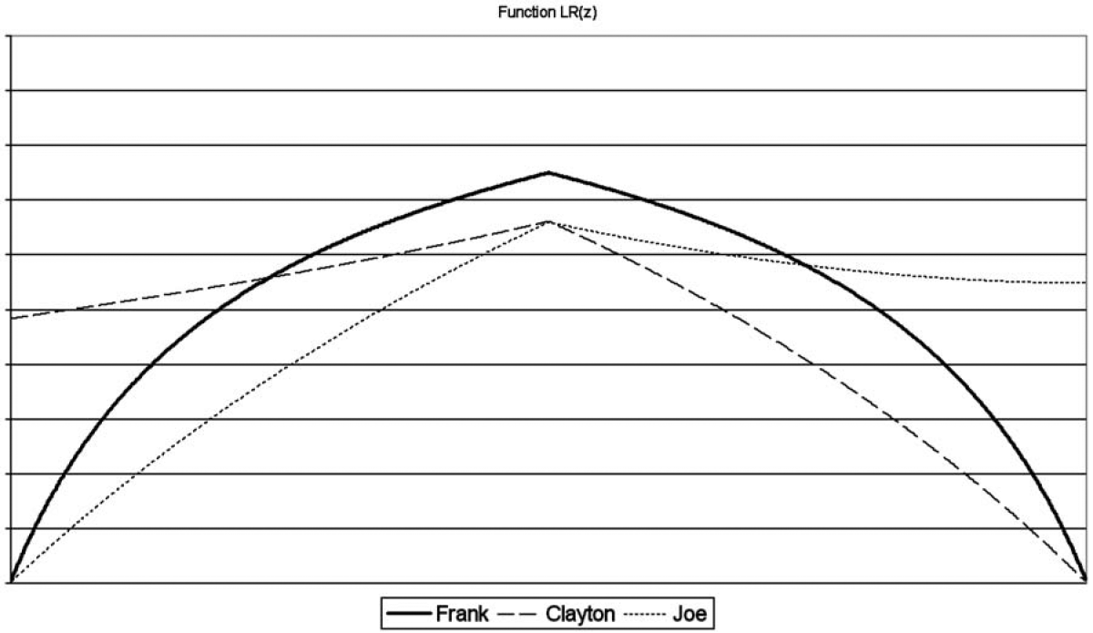
In this paper, we use three different Archimedean copulas with one parameter. There are many ways to visualize copulas, but we chose to use the tail concentration functions (Joe 1997) to focus on the dependence that can imply each copula. The tail concentration function LR(z) is constructed on left (small value) and right (large value) dependencies. Formally, with a simplification into two dimensions, say random variables U and V, this function can be expressed as

\[ L R(z)=\left\{\begin{array}{ll} L(z) & \text { if } \quad 0 \leq z<0.5 \\ R(z) & \text { if } \quad 0.5 \leq z \leq 1 \end{array},\right. \tag{7.1} \]

where the L(z) function is the probability of U < z conditionally on V < z, while R(z) is the probability of U > z conditionally on V > z. For the three copulas studied in this paper, the Frank, the Clayton, and the Joe copulas, each LR(z) is shown in Figure 1.

The Frank copula is a very popular Archimedean copula that exhibits radial symmetry without implying tail dependence. The copula can be expressed as

\[ C_{\theta}\left(u_{1}, \ldots, u_{T}\right)=-\frac{1}{\theta} \log \left[1+\frac{\prod_{i=1}^{T}\left(e^{-\theta u_{i}}-1\right)}{\left(e^{-\theta}-1\right)^{T-1}}\right] . \tag{7.2} \]

Because copulas involving more than two random variables can only imply positive dependence, the parameter θ of the Frank copula is exclusively positive. When the parameter tends toward zero, the Frank copula becomes the independence copula (Π), expressed as the product of each marginal distribution. When the parameter is going to infinity, the Frank copula reaches the upper Frechet bound (M).

As seen in the LR(z) function, the Clayton copula shows left-tail dependence, implying that a small value of one variable brings high probability of having a small value for the other one. The T-variate Clayton’s copula is expressed as

\[ C_{\theta}\left(u_{1}, \ldots, u_{T}\right)=\left[u_{1}^{-\theta}+\cdots+u_{T}^{-\theta}-T+1\right]^{-1 / \theta} . \tag{7.3} \]

As with the Frank copula, the parameter of the Clayton copula is strictly positive, Π copula is reached for θ → 0, and M copula is reached for θ → ∞.

Last, the Joe copula shows right dependence and is expressed as

\[ C_{\theta}\left(u_{1}, \ldots, u_{T}\right)=1-\left[1-\prod_{i=1}^{T}\left(1-\left(1-u_{i}\right)^{\theta}\right)\right]^{1 / \theta}, \tag{7.4} \]

where the parameter θ ≤ 1, Π copula reached for θ = 1 and M copula for θ → ∞.

7.3. Dependence

7.3.1. Exchangeable dependence

Supposing a joint distribution that is modeled by Poisson or negative binomial marginal distributions, we can suppose an exchangeable dependence based on

\[ \begin{array}{l} \operatorname{Pr}\left[N_{i, 1}=n_{i, 1}\right] \\ \quad=\operatorname{Pr}\left[N_{i, 1} \leq n_{i, 1}\right]-\operatorname{Pr}\left[N_{i, 1} \leq n_{i, 1}-1\right] \end{array} \tag{7.5} \]

and

\[ \begin{aligned} \operatorname{Pr}\left[N_{i, 1}\right. & \left.=n_{i, 1}, N_{i, 2}=n_{i, 2}\right] \\ = & \operatorname{Pr}\left[N_{i, 1} \leq n_{i, 1}, N_{i, 2} \leq n_{i, 2}\right] \\ & -\operatorname{Pr}\left[N_{i, 1} \leq n_{i, 1}-1, N_{i, 2} \leq n_{i, 2}\right] \\ & -\operatorname{Pr}\left[N_{i, 1} \leq n_{i, 1}, N_{i, 2} \leq n_{i, 2}-1\right] \\ & +\operatorname{Pr}\left[N_{i, 1} \leq n_{i, 1}-1, N_{i, 2} \leq n_{i, 2}-1\right] \end{aligned} \tag{7.6} \]

from which we use the generalization of Vandenhende and Lambert (2000) for T events to compute the contribution to the likelihood for any insured i as

\[ \begin{aligned} \operatorname{Pr}\left[N_{i, 1}\right. & \left.=n_{i, 1}, \ldots, N_{i, T}=n_{i, T}\right] \\ = & \sum_{l_{1}=n_{i, 1}-1}^{n_{i, 1}} \cdots \sum_{l_{T}=n_{i, T}-1}^{n_{i, T}}(-1)^{\sum_{j}\left(n_{i, j}-l_{j}\right)} \\ & \quad \times \operatorname{Pr}\left(N_{i, 1} \leq l_{1}, \ldots, N_{i, T} \leq l_{T}\right) \\ = & \sum_{l_{1}=n_{i, 1}-1}^{n_{i, 1}} \cdots \sum_{l_{T}=n_{i, T}-1}^{n_{i, T}}(-1)^{\sum_{j}\left(n_{i, j}-l_{j}\right)} \\ & \quad \times C\left(F_{i, 1}\left(l_{1}\right), \ldots, F_{i, T}\left(l_{T}\right)\right) . \end{aligned} \tag{7.7} \]

As for the other count distributions seen so far, the marginal distribution can be modeled with covariates. Additionally, the parameter of the copula can also be modeled with regressors, but these regressors must be time invariate since the parameter of the copula is used to model all time dependences.

This major drawback of the exchangeable dependence model is that the use of this kind of model does not allow predictions. Indeed, even if the dependence between the number of reported claims is defined for all time periods that are in the database, we cannot suppose the kind of dependence implied for periods T + j, j = 1, 2, . . . .

7.3.2. Autoregressive dependence

As for the other models seen so far, we can suppose a decreasing dependence with the time lag separating two insured periods. Following the work of Vandenhende and Lambert (2000), this autoregressive dependence is using a first-order Markov model:

\[ \begin{aligned} \operatorname{Pr}\left(N_{i, t}\right. & \left.=n_{i, t} \mid n_{i, t-1}, n_{i, t-2}, \ldots\right) \\ = & \operatorname{Pr}\left(N_{i, t}=n_{i, t} \mid n_{i, t-1}\right) \\ = & \operatorname{Pr}\left(N_{i, t} \leq n_{i, t} \mid n_{i, t-1}\right) \\ & -\operatorname{Pr}\left(N_{i, t} \leq n_{i, t}-1 \mid n_{i, t-1}\right), \end{aligned} \tag{7.8} \]

where the probability can be expressed as a function of a bivariate copula:

\[ \begin{array}{l} \operatorname{Pr}\left(N_{i, t} \leq n_{i, t} \mid n_{i, t-1}\right)= \\ \quad \frac{C\left[F_{t-1}\left(n_{i, t-1}\right), F_{t}\left(n_{i, t}\right)\right]-C\left[F_{t-1}\left(n_{i, t-1}-1\right), F_{t}\left(n_{i, t}\right)\right]}{\operatorname{Pr}_{t-1}\left(N_{i, t-1}=n_{i, t-1}\right)}, \end{array} \tag{7.9} \]

and the contribution to the likelihood of each insured i can be written as

\[ \begin{array}{l} \operatorname{Pr}\left[N_{i, 1}=n_{i, 1}, \ldots, N_{i, T}=n_{i, T}\right] \\ \quad=\operatorname{Pr}\left(N_{i, 1}=n_{i, 1}\right) \prod_{j=2}^{T} \operatorname{Pr}\left(N_{i, j}=n_{i, j} \mid n_{i, j-1}\right) . \end{array} \tag{7.10} \]

Covariates can also be used to model the marginal distributions, but as opposed to the exchangeable dependence model, time-varying covariates can be used to model the parameters of the copula, using appropriate transformations that respect their domains. While marginal moments can be found directly with their marginal distribution (Poisson or negative binomial distributions), conditional moments cannot be expressed in a closed form. Use of Equations (7.8) to (7.10) is needed to compute such moments.

7.4. Predictive distribution

The autoregressive dependence model defined the predictive distribution directly. It only depends on the number of reported claims of the last insured period.

7.5. Numerical application

Estimated parameters of the data applied to the copula models with Poisson and NB1 marginal distributions are exhibited in Tables 6 and 7. Clearly and without surprise, we see that the copulas applied to NB1 distribution result in a log-likelihood smaller than the one obtained by the Poisson marginals.

Parameters’ estimates are quite the same as those observed in other models. An interesting observation is the fit exhibited by each copula since the Joe copula with NB1 marginal seems to exhibit a better adjustment to the data. Remember that this copula has a tail dependence at the right, meaning that an insured with a high number of reported claims in a year will see an increase in his expected number of reported claims for the next year.

8. Model comparisons

Differences between models can be analyzed through the mean and the variance of some insured profiles. The mean corresponds to the frequency part of the a priori premium, that is to say, premiums for new insureds. Three profiles, as displayed in Table 8, have been analyzed. The exogenous variables v1, . . . , v5 were described in Table 1.

The first profile is known to be a good risk, while the last profile usually exhibits bad loss experience the other profile is medium risk. Table 9 shows quite similar premiums for all models, where the biggest differences for the expected values are exhibited by the artificial marginal (AM) and the Frank copula models. Because the estimations of the parameters are approximately the same for all models, this result was expected since the sufficient conditions for consistency are satisfied (Gourieroux, Monfort, and Trognon 1984a, 1984b). Nevertheless, other elements can be analyzed, such as the variance values, which is important in some forms of premium calculations and solvency analysis that show greater variations between models.

For an insured with a claim, the expected value or the predictive premiums are based on the number of reported claims of the last insured period, as shown in Tables 10 and 11 for the medium risk profile. The time-independent models are not shown, since the expected value as well as other property of this distribution do not depend on past claims. As opposed to a priori premiums, we see that the choice of a model greatly influences the values of predictive premiums. Indeed, the ratio increase between the smallest and the largest predictive premiums is approximately 4% for a claim-free driver, goes to more than 40% for an insured who reported one claim in his last insured period, goes to 108% for two reported claims, and attains more than 800% for a four-claims reporter, that is to say, in this case, that the largest premium is nine times larger than the smallest one.

Since it is not based on autocorrelation of order one, as opposed to other models, the random effects models do not only depend on the number of reported claims of the last insured period but on the sum of all reported claims. For example, for a driver with a history of 10 years, the predictive premiums of those models are those shown in Table 12. This property of the random effects model must be seen as a great advantage over the other models since the unobserved characteristics of the driver are not only shown by his last insured period, but by all his claim experience.

9. Link between models

As shown in the preceding sections, there are links between some of the models. For specific parameter restrictions, some models are nested, such as Poisson and negative binomial and their generalizations that account for time dependence or Poisson-based models against their negative binomial-based generalization. On the other hand, some models are non-nested to each other, such as the link between all models allowing for time dependence. Though it is not the primary purpose of this paper, many possible tests are shown in this section to assess the model fit.

9.1. Nested models

Two situations imply nested models for the distributions seen on this paper. First, to account for overdispersion of the marginal distribution, the Poisson distribution has been generalized into negative binomial distribution in all models allowing for time dependence. The way to test this generalization is to check if the extra parameter accounting for the overdispersion is statistically significant. Secondly, other nested models are the time-independent models and their generalizations into models where time dependence exists, like the Poisson against its generalization into Poisson-INAR(1). As for the overdispersion test, it can be done by a check on the extra parameter that implies the time dependence.

One problem with standard specification tests (Wald or likelihood ratio tests) happens when the null hypothesis is on the boundary of the parameter space. When a parameter is bounded by the H₀ hypothesis, the estimate is also bounded and the asymptotic normality of the maximum likelihood estimation no longer holds under H₀. Consequently, a correction must be done. Results from Chernoff (1954) for the likelihood ratio statistic and Moran (1971) for the Wald test, reviewed by Lawless (1987) for the study of the negative binomial distribution, showed that under the null hypothesis, the LR statistic has a probability mass of \(\frac{1}{2}\) on the boundary and a \((1 / 2) \chi_{1-2 \delta}^2\) (rather than \(\chi_{1-\delta}^2\) ) distribution. Consequently, in this situation, a one-sided test must be used. An analogous result shows that for the Wald test, there is a mass of one half at zero and a normal distribution for the positive values. In this case, as mentioned by Cameron and Trivedi (1998), one continues to use the usual one-sided test critical value of \(z_{1-\delta}\).

Another way to deal with this is to use tests that do not change properties under this kind of hypothesis, such as score tests (Moran 1971; Chant 1974) or Hausman (1978) test. However, testing these overdispersion situations for time-dependent models or testing the parameter that implies time dependence has not been the subject of much research until now. Consequently, in our situations, we will base our results on adapted standard tests of Wald and likelihood ratio tests, even if we know that some improvements must be done in this area.

For more details about these tests, or other ones, refer to Cameron and Trivedi (1998) or Winkelmann (2003) in the context of count data or Gourieroux and Monfort (1995) for a general point of view. For actuarial applications of count data when independence between contracts of the same insured is supposed, see Boucher, Denuit, and Guillén (2007).

9.1.1. Numerical application

Three kinds of links can be tested by the tests of nested models:

• Overdispersion test as Poisson marginal against negative binomial marginal;^[2]

• Poisson against their generalized models allowing for time dependence;

• Negative binomial against their generalized models allowing for time dependence.

Direct application of Wald and likelihood ratio tests can be done on all models seen in this paper. The results are quite clear: all Poisson marginals are rejected against their overdispersed generalization, all Poisson and negative binomial distributions are rejected against their generalized models allowing for time dependence. All these tests involve p-values less than 0.01%.

9.2. Non-nested models

Apart from the comparison between models where the marginal distribution is Poisson or negative binomial, the other models can be seen as non-nested models. Two kinds of non-nested models exist: overlapping and strictly non-nested models. Overlapping models refer to models where neither model can be derived from the other by parameter restriction, but where some joint parameter restrictions result in the same model. Strictly non-nested models refer to models where even conjoint parameter restriction cannot produce identical models. For a general discussion on non-nested models or for more formal definitions of non-nested models, see Pesaran (1974) and Vuong (1989).

9.2.1. Information criteria

Standard methods of comparing non-nested models refer to the information criteria, based on the fitted log-likelihood function. Since the log-likelihood increases with the addition of parameters, the criteria used to distinguish models must penalize models with a large number of parameters. Developments of such methods began with the work of Akaike (1973) and Schwartz (1978), who proposed the Akaike information citeria on (AIC) = −2 log(L)+ 2k and the Bayesian information criteria on (BIC) = −2 log(L) + log(n)k, where k and n represent respectively the number of parameters of the model and the number of observations. Many other penalized criteria have been proposed in the statistical literature [see Kuha (2004) for an overview]. However, the AIC and BIC criteria are the most often used in practice. Application of these criteria on the nonrejected models seen in the first section leads to the results of Table 13.

Models do not contain the same number of parameters. Consequently, analysis of each information criteria can result in different conclusions. Note that despite their apparent simplicity, the information criteria are based on explicit theoretical considerations, and AIC and BIC do not have the same foundations. As shown by Kuha (2004), referring to older papers such as Atkinson (1981) and Chow (1981), the aims of the AIC and BIC criteria are not the same. The aim of the BIC, referring to a Bayesian approach, is to identify the model with the highest probability to be true, given that one model under investigation is true. On the other side, the AIC denies the existence of an identificable true model and, for example, minimizes the distance or discrepancy between densities. Moreover, in model selection, it has been argued that the BIC criteria penalizes large models too heavily. However, unsurprisingly, results of the previous table clearly show that the random effects models are better to model the insurance data than the other models seen in this paper. More particularly, we see that the NB1-beta model is the model that provides the better fit to our data.

This analysis can be illustrated differently. Indeed, we can do an intuitive analysis of the log-likelihood by models, by separating this statistic by year. To smooth the random variations between year, we analyze and illustrate the cumulative difference of fit between each remaining model and the Poisson distribution, which does not imply dependence between contracts of the same insured. Because the models do not involve the same number of parameters, a correction factor AIC is also used. Figure 2 shows the values of a pseudo-AIC by year (versus the Poisson distribution) for each of the remaining models presented.

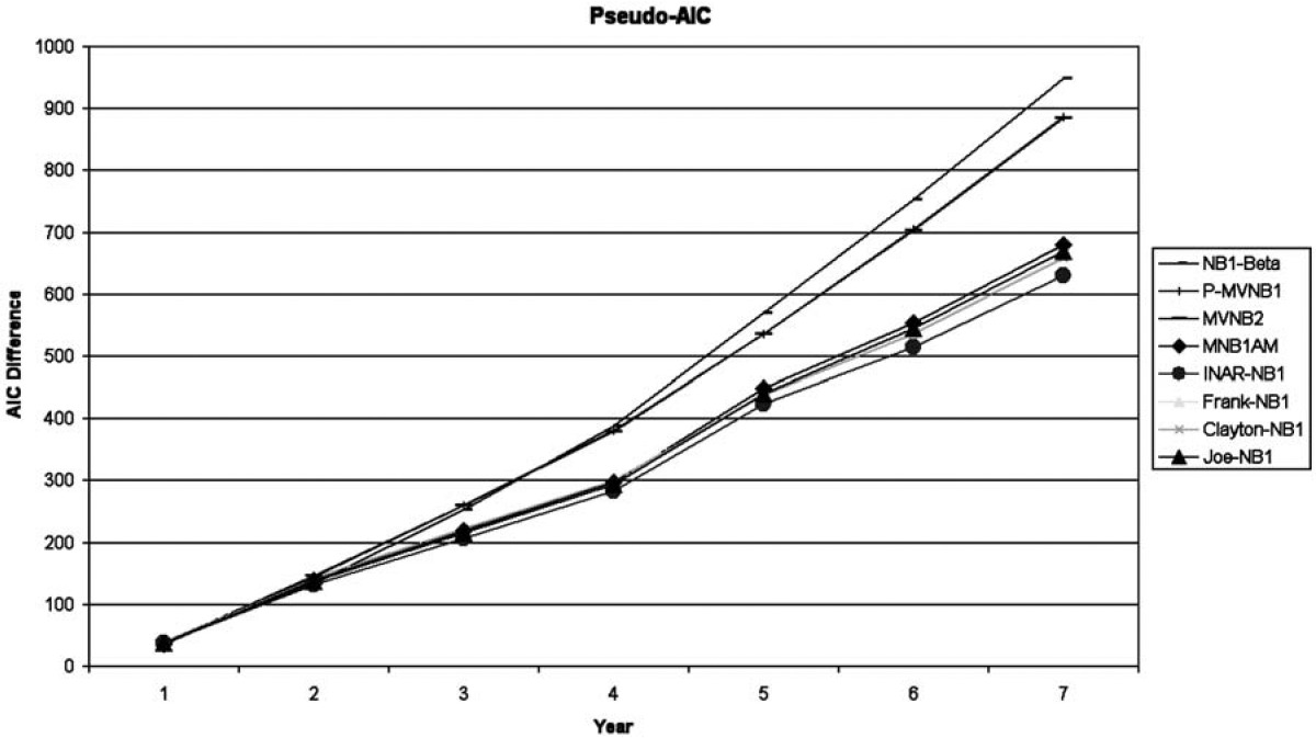
As the number of experience years grows, we can see that the fits of the random effects models are clearly better than the Poisson distribution. Indeed, as the past experience increases, other models show their limited predictive capacity, because the improvement in the fit stays proportional with the number of years, as they are only based on the number of claims of the last insured period. By opposition, the random effects models seem to improve more and more in their fit as the number of insured periods grows.

9.2.2. Vuong test

Random effects models clearly show a better fit than the other models. To see if the difference in the log-likelihood between the MVNB model (which shows approximately the same fit as the Pseudo MVNB1) and the NB1-beta model is statistically significant (as illustrated in the seventh year of the last graph), a test based on the difference in the log-likelihood can be performed.

For independent observations, a log-likelihood ratio test for non-nested models developed by Vuong (1989) and generalized by Rivers and Vuong (2002) can be used to see if the NB1-beta model is statistically better than the other models. This test is based on the likelihood ratio approach of Cox (1961), with a correction that corresponds to the standard deviation of this difference. As opposed to Boucher, Denuit, and Guillén (2007), who applied directly the Vuong test on all available models, this test cannot be applied directly on our models since some observations—all contracts of the same insured—are not independent. However, as proposed by Golden (2003), this non-nested models test can be generalized quite directly to correlated observations. It can be expressed as

\[ T_{L R, N N}=\frac{\sqrt{n T}\left(\sum_{i} \sum_{t} \ell\left(f_{i, t}, \hat{\beta}_{1}\right)-\ell\left(g_{i, t}, \hat{\beta}_{2}\right)\right)}{\sigma_{T_{L R, N N}}},\tag{9.1} \]

where the log-likelihood function for the distribution ƒ is defined as

\[ \ell\left(f_{i, t}, \hat{\beta}_{1}\right)=-\log \left[P_{f}\left(n_{i, t} \mid n_{i, t-1}, \ldots, n_{i, 1}\right)\right]. \tag{9.2} \]

Then, for observation at time \(t\), conditional log-likelihood must be expressed based on experience \(1,2, \ldots, t-1\), using predictive distributions. The parameter \(\sigma_{T_{L R, N N}}\) is the square root of the discrepancy variance and is expressed as:

\[ \begin{aligned} \sigma_{T_{L R, N N}}^{2}= & \frac{1}{n} \sum_{i=1}^{n} \sum_{t=1}^{T} \sum_{j=1}^{T}\left(\ell\left(f_{i, t}, \hat{\beta}_{2}\right)-\ell\left(g_{i, t}, \hat{\beta}_{2}\right)\right) \\ & \times\left(\ell\left(f_{i, j}, \hat{\beta}_{2}\right)-\ell\left(g_{i, j}, \hat{\beta}_{2}\right)\right). \end{aligned} \tag{9.3} \]

The expression of the variance is closely related to the one obtained with the standard Vuong test, except that the covariances between correlated observations are considered. Note that even if the generalization of this test for correlated observations share close similarities to the Vuong test, intermediary tests must be performed to ensure that the test is valid (Golden 2003). First, a necessary but not sufficient condition to establish asymptotic properties of this test involves the calculation of the following matrix:

\[ B=\left[\begin{array}{ll} B_{f, f} & B_{f, g} \\ B_{g, f} & B_{g, g} \end{array}\right], \tag{9.4} \]

where

\[ B_{f, g}=\frac{1}{n}=\sum_{i=1}^{n} \sum_{t=1}^{T} \sum_{j=1}^{T} \nabla \ell\left(f_{i, t}, \hat{\beta}_{1}\right) \nabla \ell\left(g_{i, j}, \hat{\beta}_{2}\right). \tag{9.5} \]

The matrix \(B\) must be positive definite or, at least, must converge to it [see Golden (2003) for details]. Since the variance of the difference between log-likelihood involves covariance terms, the second intermediary step is done to avoid a situation where \(\sigma_{T_{L R, N N}}\) can be equal to zero. It involves the calculation of the estimated discrepancy autocorrelation coefficient and is defined as:

\[ \hat{r}=\frac{\sum_{i=1}^{n} \sum_{t=1}^{T} \sum_{j=1, j \neq t}^{T}\left(\ell\left(f_{i, t}, \hat{\beta}_{1}\right)-\ell\left(g_{i, t}, \hat{\beta}_{2}\right)\right)\left(\ell\left(f_{i, j}, \hat{\beta}_{1}\right)-\ell\left(g_{i, j}, \hat{\beta}_{2}\right)\right)}{2 T \sum_{i=1}^{n} \sum_{t=1}^{T}\left(\ell\left(f_{i, t}, \hat{\beta}_{1}\right)-\ell\left(g_{i, t}, \hat{\beta}_{2}\right)\right)^{2}} \tag{9.6} \]

The adapted test of Golden (2003) assumes that \(\hat{r} \neq-1 /(2 T)\), so this assumption must be verified to ensure that the test is correctly specified. The last intermediary test verifies that the two models cannot be equal. Since we work with non-nested models and we already verify that models cannot be equal by simultaneous parameter restrictions, this step is not needed in our case.

To apply the adapted Vuong test for correlated observations, neither of the two models has to be true. The null hypothesis of the test is that the two models are equivalent, expressed as \(H_0\) : \(E\left[\ell\left(f, \hat{\beta}_1\right)-\ell\left(g, \hat{\beta}_2\right)\right]=0\). Under the null hypothesis, the tests converge to a standard normal distribution. Rejection of the test in favor of the distribution \(f\) happens when \(T_{L R, N N}>c\), or in favor of \(g\) if \(T_{L R, N N}<c\), where \(c\) represents the critical value for some significance level.

Modification of this test is needed in the case where the compared models do not have the same number of parameters. As proposed by Vuong (1989), we may consider the following adjusted statistic:

\[ \hat{C}(\theta)=C(\theta)+K(f, g). \]

where K(ƒ,g) is a correction factor based on the difference between the information criteria (seen in the preceeding subsection) of models ƒ and g.

For the MVNB against the NB1-beta models, the Vuong test, adapted to correlated observations, shows that the NB1-beta model is statistically better than the MVNB model. Indeed, the resulting test involves a p-value of less than 0.5% for the adapted tests (AIC and BIC). Intermediary tests show that the matrix B is positive definite, while the value of the estimated discrepancy autocorrelation coefficient is far from − 1/14 since it equals 0.07.

10. Conclusion

A wide selection of models can be used to model the dependence that can exist between contracts of the same insured, and each model can be interpreted differently. We showed that the choice of a model has a great impact on the predictive premiums, that is to say, premiums based on claim experience. We also showed that, despite their initial intuitive appeal, some models cannot be used. We conclude that the random effects models are the better ones to fit the data since they are more flexible to compute the next year premium, with dependence not only on the past insured period but on the sum of all reported claims. More precisely, we saw that the NB1-beta model exhibits statistically the better fit. Formally, this choice of the best distribution describing our data has been supported by specification tests for nested or non-nested models.

All the models analyzed were based on generalizations of Poisson and NB1 distributions. Models seen in this paper could be applied on other claim count distributions, such as Hurdle or zero-inflated models that provided good fit for cross-section data (Boucher, Denuit, and Guillén 2007). A study in the vein of the present one could also be performed for claim severities to propose interpretations of the process that generates the dependence between claim amounts.

---

1. We do not call this model multivariate negative binomial or negative multinomial distributions, since these names refer to Poisson distributions sharing the same heterogeneity variable, as seen in Section 3.

2. Note that the Poisson random effects model is not nested to the negative binomial distribution with random effects.