Using Dynamic Linear Models with Changepoints to Understand Trends in the Auto Insurance Industry

1. Introduction

The personal auto insurance industry is constantly changing. There are small but constant changes over time (e.g., inflation affecting the cost of repairs and general progress in the safety of vehicles) and sharp spikes (e.g., disasters and legislation). Change has never been more apparent than with the COVID-19 pandemic, civil unrest, and driverless cars all presently having or soon to have significant impacts on personal auto insurance. While our data does not include enough detail after the start of the pandemic to explicitly examine those impacts, the rapidly changing world shows the necessity of a flexible model.

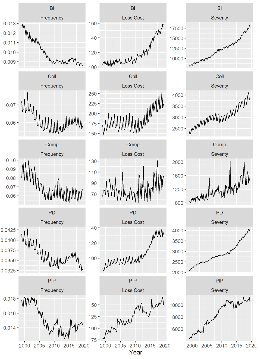
Looking at our data, personal auto insurance frequency (number of claims per covered car year) had been consistently falling for many years prior to the financial crisis (2008–2010). This trend is largely attributed to improvements in collision avoidance technology, increased safety awareness, and changes in enforcement. Since the financial crisis, countrywide frequency has remained relatively constant. Both collision (Coll) and property damage (PD) frequency seemed to increase from 2010 to 2016 before falling to the present. Countrywide severity (total loss per claim) has increased exponentially rather consistently since 1999, though there might have been some slowing around the financial crisis, especially in PD and Coll. Countrywide loss cost (total loss per covered car year) is a combination of frequency and severity. Bodily injury (BI), PD, and Coll all were fairly constant (with falling frequency and increasing severity canceling each other out) until the financial crisis, and they have been increasing significantly since then. Personal injury protection (PIP) has increased fairly steadily, and comprehensive (Comp) has stayed constant. Figure 1 plots all three metrics on a countrywide level.

Figure 1.Countrywide frequency, severity, and loss cost, Q1 1999 through Q3 2019.

In addition to the overall trends, there are obvious seasonal patterns for frequency, severity, and loss cost. A typical model choice for time series data such as this would be an AR, ARMA, or ARIMA model with a seasonal component. However, the shifts or changepoints in the data—as is apparent when looking at the plots of frequency, severity, and loss cost—suggest that a structural change should be incorporated directly into our model.

The practice of determining shifts in the structure of time-dependent data starts with Sen and Srivastava (1975) and Hawkins (1977). Many methods have been proposed over the years, including nonparametric methods (Miao and Zhao 1988; Darkhovski 1994), combining with ARCH and GARCH time series models (Kokoszka, Leipus, and others 2000; Kokoszka, Teyssière, and others 2002), and considering multiple changepoints (Braun, Braun, and Müller 2000; Hawkins 2001). While these methods typically focus on detecting changepoints in the mean structure, models with changepoints in the covariance structure have also been used (Chen and Gupta 2004).

The main modeling tool we use in this paper is a dynamic linear model (DLM) (West and Harrison 2006; Prado and West 2010). A DLM is a very powerful tool as it allows for a realistic separation of the underlying process from the observed noisy data. Parameters that switch over time have been thoroughly explored in DLMs (Shumway and Stoffer 1991; Kim 1994). Especially popular are time-varying autoregressive structures in DLMs (Prado, Huerta, and West 2000). These models typically focus on having two or more regimes where regime assignment is time-dependent. This class of models does not meet our purpose of determining distinct trends before and after a fixed point in time. More applicable changepoint models are found in Whittaker and Frühwirth-Schnatter (1994), Daumer and Falk (1998), and Park (2006). Each of these models varies different components of the DLM structure to achieve a changepoint effect. We introduce another simple yet different approach to changepoint modeling in DLMs that essentially treats time as a regression variable and allows the coefficient to change at some point in the process.

2. Data

The loss data is gathered from the Fast Track Plus database from the Independent Statistical Service. We obtained quarterly loss amounts, claims, and earned car years for each state and coverage (BI, PD, Comp, Coll, PIP, and property protection [PPI]) from Q1 1999 through Q3 2019. Because of our date range, we will not be able to infer any impacts of the current public health crisis or social unrest. We then calculated frequency (claims / earned car years), severity (loss amount / claims), and loss cost (loss amount / earned car years). For the remainder of this report, we focus on those three metrics.

In addition to the loss data, we gathered congestion data from the Federal Highway Administration (an agency within the U.S. Department of Transportation that supports state and local governments in the design, construction, and maintenance of the nation’s highway system). We defined congestion as vehicle miles traveled / total road miles. We subset this data to include only urban roads, only rural roads, and all roads. One shortcoming of this information is that it is only provided at the annual level, so we assumed that all quarters are the same within the year. We compared the results to a smoother interpolation and found that it did not have a noticeable impact.

3. Methods

A DLM is characterized by two levels of modeling. The higher level connects the data, $Y_t$, to latent unobserved state variables, $\theta_t$, which is often a vector. The lower level models the evolution of the state variables over time. This can be expressed as

$$\begin{aligned} Y_t &=& F_t \theta_t + \nu_t, ~~ \nu_t \sim N(0,v),\end{aligned}\tag{1}$$

$$\begin{aligned} \theta_t &=& G_t \theta_{t-1} + \omega_t, ~~ \omega_t \sim N(0,W). \end{aligned}\tag{2}$$

The vector $F_t$ and matrix $G_t$ control the dynamics of the model. The specific formulation of these matrices is crucial to properly fitting the model. The scalar parameter $v$ and matrix $W$ denote the observational noise and process noise, respectively.

For our specific model, the state vector is composed of four pieces: (1) polynomial model of order 1, which is essentially a random walk component; (2) four-period seasonal trend; (3) regression trend; and (4) linear trend with a changepoint. These components are represented by the following DLM structure:

$$F_t=\left(1,1,0,0, X_t, t, t Z_t\right) \tag{3}$$

$$G_t=G=\operatorname{diag}\left(1,\left(\begin{array}{ccc} 1 & 1 & 1 \\ -1 & 0 & 0 \\ 0 & -1 & 0 \end{array}\right), 1,1,1\right) \tag{4}$$

The variable $X_t$ represents congestion at time $t$, and $Z_t$ is an indicator variable that is 0 when $t$ is less than the changepoint and 1 when $t$ is greater than the changepoint. This linear trend is essentially a linear spline where the slope changes at the changepoint. The process noise covariance matrix is $W = \mbox{diag}(\eta_1,\eta_2,0,0,\eta_3,0,0)$, which allows the polynomial, seasonal, and regression effects to vary over time.

If the state vector is $\theta_t = (\theta_{t,1},...,\theta_{t,7})'$, then the regression coefficient for the congestion variable is $\theta_{t,5}$. The slope of the linear trend is $\theta_{t,6}$ prior to the changepoint and $\theta_{t,6} + \theta_{t,7}$ after the changepoint.

The unknown parameters that need to be estimated in the model include the state variables $\theta_t, t= 1,...,T$ and the variance variables $v, \eta_1, \eta_2$, and $\eta_3$. These can all be estimated using a Markov chain Monte Carlo algorithm with a process called forward filtering backward sampling (FFBS) (Frühwirth-Schnatter 1994; Carter and Kohn 1996). Essentially, this algorithm draws samples for the state variables given current estimates of the variance terms; then the variance terms are estimated conditional on the sampled state vectors. Sampling the state vectors uses standard filtering formulas, which are derived from the full normal conditionals of the state vectors. The variance terms can be sampled conjugately when given inverse gamma priors with parameters $\alpha$ and $\beta$. The posterior distribution for each of these variables is given below. Let $\mathbf{Y} = (Y_1,...,Y_T)$ and $\theta = (\theta_0',...,\theta_T')$ represent the data and state vectors for all time points.

$$\small{ \begin{aligned} v|\mathbf{Y}, \theta \sim& IG\left(\alpha+T/2,\beta + \frac{1}{2}\sum_{t=1}^T(Y_t- F_t \theta_t)^2\right)\end{aligned} \tag{5}}$$

$$\small{ \begin{aligned} &\eta_b|\mathbf{Y}, \theta \sim IG\left(\alpha+T/2,\beta+\frac{1}{2}\sum_{t=1}^T(\theta_{t,b}-\theta_{t-1,b})^2\right), \\ &\quad b = 1,2,3 \end{aligned}\tag{6}}$$

This particular structure was chosen for the auto loss cost data specifically by testing a number of different models on a subsample of the time series. The main feature of the model is the linear trend that accounts for a potential changepoint. There are many different types of models that could be used to account for a change in dynamics at a specific point in time. Additional or different features could have been added to the model as well. Following are structures for the time-varying component that were tested for the data; components such as the regression and seasonal effects were included in all models:

• Time-varying autoregressive structure with a fixed regime before and after the changepoint (Prado, Huerta, and West 2000)

• Two polynomial models of order 1 before the changepoint and a polynomial model of order 2 after the changepoint (Daumer and Falk 1998)

• Different polynomial models of order 2 before and after the changepoint

• Linear and quadratic regression terms in time

Each of these models is in fact more complicated in structure than the one we are using. However, on the subsample of time series tested, the simpler model we are using gives the best energy score every time.

To test many different types of model structures, a continuous rank probability score was used, which is also called an energy score (Gneiting and Raftery 2007). An energy score is a metric that compares multiple samples from a posterior predictive distribution against the data. A better fitting model will have a lower energy score. The formula for an energy score using $m$ samples from the posterior predictive distribution is

$$\small{ \begin{align} E S=\frac{1}{m} \sum_{i=1}^m\left\|\boldsymbol{Y}-\boldsymbol{Y}^{(i)}\right\|-\frac{1}{2 m^2} \sum_{i=1}^m \sum_{j=1}^m\left\|\boldsymbol{Y}^{(i)}-\boldsymbol{Y}^{(j)}\right\| . \end{align} \tag{7} }$$

Energy scores are able to account for distributional fit as well as predictive error. Specifically, the posterior predictive draws for one-step ahead predictions of every time point conditional on only previous time points is compared against the truth. It penalizes for model complexity, ensuring that selected changepoints are important and preventing overfitting. It is often preferred over other metrics such as the deviance information criterion for Bayesian stochastic processes (Cressie and Wikle 2015). In this particular application, we expect the ordering of model fits using energy scores to be similar to what a deviance information criterion would provide.

Energy scores will also be used to determine other aspects of the final models for each time series, such as which changepoint to use, which congestion variable is most predictive, and whether to use a congestion variable or changepoint at all. When no congestion variable or no changepoint is used, the model structure is different, as summarized in the following subsections.

No changepoint and no congestion parameter

The simplest of all these models is the one with no changepoint included and no regression parameter for congestion. In this case, equations 3 and 4 are modified to remove the components relating to the changepoint and regression terms. This results in

$$F_t = (1,1,0,0,t)$$

and

$$G_t = G = \mbox{diag}\left(1, \left(\begin{array}{ccc}1 & 1 & 1 \\ -1 & 0 & 0 \\ 0 & -1 & 0 \end{array}\right),1\right).$$

This includes a constant linear trend, a polynomial trend, and a seasonal trend. There is only one such model for each times series. In the case with no regression coefficient, $\eta_3$ is also removed from the model and will not need to be estimated.

No changepoint with congestion parameter

The model with no changepoint but with the congestion parameter as a regression term has dynamics of $$F_t = (1,1,0,0,X_t,t)$$ and $$G_t = G = \mbox{diag}\left(1, \left(\begin{array}{ccc}1 & 1 & 1 \\ -1 & 0 & 0 \\ 0 & -1 & 0 \end{array}\right),1,1\right).$$ With three congestion parameters compared, this comprises three of the total number of models run per time series.

With changepoint and no congestion parameter

The model with a changepoint and no congestion variable has dynamics of

$$F_t = (1,1,0,0,t,t Z_t)$$

and

$$G_t = G = \mbox{diag}\left(1, \left(\begin{array}{ccc}1 & 1 & 1 \\ -1 & 0 & 0 \\ 0 & -1 & 0 \end{array}\right),1,1\right).$$

There is one model produced by this structure for every changepoint examined.

The model that has both a changepoint and congestion parameter is given in equations 3 and 4. With three possible regression terms, the number of models this structure produces is three times the number of changepoints examined.

4. Results

As mentioned above, fitting a single model to a wide range of data is a difficult task. We have a rather large and varied dataset with

• 229 state and coverage combinations

  • 52 states each, all 50 states + DC + countrywide for BI, PD, Comp, and Coll

  • 20 PIP states

  • 1 PPI state (Michigan);

• three different metrics: frequency, severity, and loss cost;

• four different congestion possibilities: total, urban, rural, and none (except DC does not have rural areas, so no rural congestion values); and

• 52 different possible changepoints and one model without a changepoint.

This makes a total of $(229 * 3 * 4 - 15) * 53 = 144,849$ possible models to compare. Each model took about 5 minutes to run, for about 1.5 years of total compute time. Luckily, it is easily parallelized, taking only about a week of elapsed time.

Because the posterior distributions of the parameters have closed form distributions, no Metropolis–Hastings is needed for the parameter estimation. Posterior convergence was not checked on every model, but for every model that was checked, convergence was achieved quickly and easily as indicated by visual inspection of the trace plots.

To parse through these results, we will first describe overall trends in the results, which we will solidify with a few examples. For those combinations where the model did poorly, we will outline potential next steps to overcome the issues. Results from all the combinations are available in the online appendix.

Energy scores are used to compare each model fit on the individual time series. The model that has the lowest energy score is denoted as the optimal model. As we display the time series plots, we will not only designate where the optimal changepoint is but also the second and third optimal changepoints. This helps give a broader understanding of possible periods where the time series has a structural shift.

4.1. Individual time series trends

The purpose of these results is to assess structural changes in the auto insurance trends. For example, one can use these results to see if there is a significant shift during or after the financial crisis from 2008 to 2010. We have included two selections from the online appendix (for Tennessee and Virginia) in Figure 2. Using these two selections as examples, we will describe how to use the results in the appendix to draw conclusions about auto insurance trends.

Figure 2.Selection from appendix for two combinations out of all state, coverage, and metric combinations.

The left plot shows the time series, and the right plot has the energy scores for fitting the time series. The different colors on the right plot represent different congestion variables. As lower energy scores represent a better model fit, the color that is the lowest on the plot represents the best congestion variable. For the Tennessee Coll loss cost, the best congestion variable is rural congestion, while for Virginia Comp loss cost, the best congestion variable is total congestion.

The dotted lines represent the energy score with no changepoint. Energy scores are plotted by possible changepoints across the x-axis. A distinctly low value on the energy score plots is a strong indication that a changepoint has improved the model fit. For example, in the Tennessee Coll loss cost energy score plot, there is a distinct downward spike around 2009. This suggests a changepoint near 2009. For Virginia Comp loss cost, there are no values that stand out as significant changepoints. There are energy scores lower than the value with no changepoints, but the energy scores for all changepoints and for no changepoints are similar, suggesting there is not strong evidence for a changepoint in this case.

As there are hundreds of these plots, it is difficult to describe possible inferences for every combination, so we leave that to the reader for any grouping they are interested in. For example, one could look at the coverages for a particular state to determine whether there were some coverages that were influenced by the financial crisis more than others. Or one could look at a specific coverage to see which states have significant structural changes.

4.2. Overall trends

We divide the discussion on the overall trends into several subsections. First, we will discuss the changepoint results, followed by the slopes of the linear trends, and finally the congestion measures.

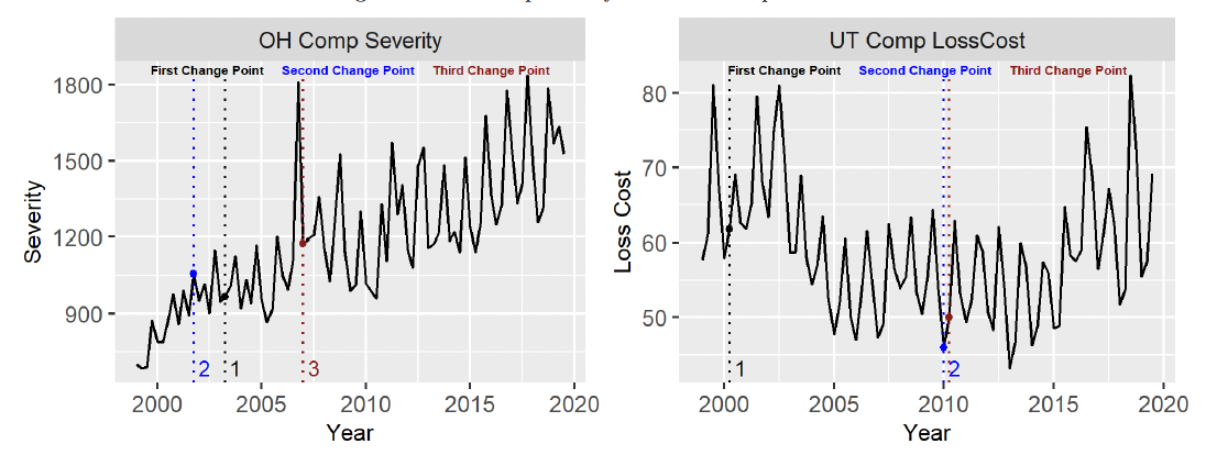
Changepoints. Almost all the state/coverage/metric combinations chose a model with a changepoint as the optimal model. The only two that did not include a changepoint are Ohio Comp severity and Utah Comp loss cost. Plots of both those values are included in Figure 3. With Ohio Comp severity, the pattern is rather consistent throughout the period, with an outlier in 2007 Q1. The magnitude of the seasonal trend does appear to increase after the outlier. For simplicity, we only allowed the overall slope of the model to change before and after the changepoint. If we had included the seasonality in the changepoint, we likely would have found a changepoint around 2007 Q1. For Utah Comp loss cost, the trend is interesting. There appears to be no steadily increasing trend but rather three constant mean periods. The first is between 1999 and about 2004 with an annual mean around 70. Then, from 2004 until 2015, the mean drops to around 55. After 2015, the mean bounces back up to around 63. Our model likely would have caught this pattern if it had allowed for two separate changepoints. As we discuss the models further, that will be a common theme: Another changepoint or two would likely change the results dramatically.

Figure 3.Ohio Comp severity and Utah Comp loss cost.

When we started this project, we thought that many of the changepoints would be chosen around the financial crisis. Table 1 shows that only slightly more optimal changepoints occurred during the financial crisis. The total proportion of models with changepoints selected in the financial crisis was only slightly more than would have been selected at random. Originally this result was disappointing. Upon closer visual investigation, however, it seemed that there were many instances of structural shifts in periods other than the financial crisis. For time series that shifted around the financial crisis, like countrywide Coll loss cost or California PD frequency, our model chose those time periods to include a changepoint (Figure 4). However, most of the datasets did not include a significant change around the financial crisis or had a more significant changepoint elsewhere. This result does not suggest a faulty model but rather suggests that major structural shifts over the 20-year period of study were not limited to the financial crisis.

Figure 4.Countrywide (CW) Coll loss cost and California PD frequency.

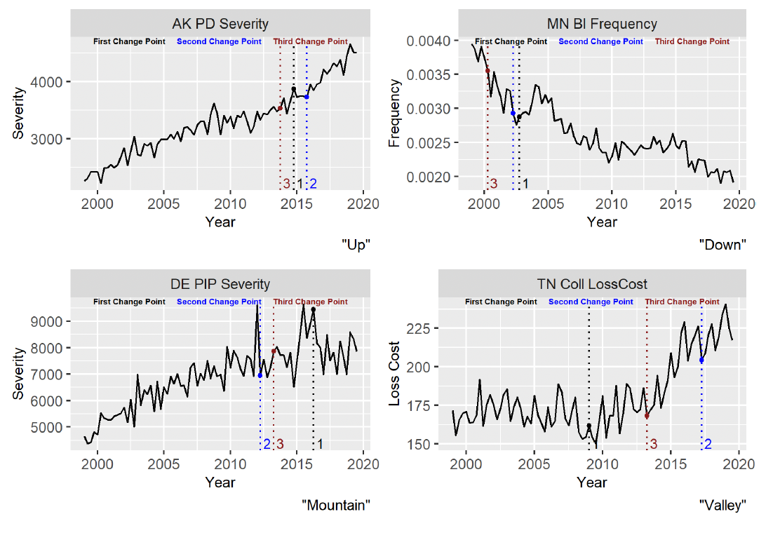
Slopes. We describe the chosen slopes of the model by dividing them into four categories (Table 2).

As examples of each type of slope, Figure 5 shows Alaska PD severity (Up), Minnesota BI frequency (Down), Delaware PIP severity (Mountain), and Tennessee Coll loss cost (Valley). Notice that the classification of the slope would change if the second- or third-best changepoint were chosen instead of the best.

Figure 5.Plots exemplifying each type of slope.

The linear slopes were largely driven by the metric. Most of the frequency models are Down and most of the severity models are Up. The combination of the two (loss cost) is mainly Up, with a large number showing a Valley (Table 3).

Congestion. In previous studies, congestion consistently rated as one of the most important variables when trying to predict statewide losses (Society of Actuaries 2020). This exercise proved to be no different. The best model had no congestion variable in 10% of the combinations. Not counting PPI, urban congestion was consistently the variable most often chosen. The proportion of models by coverage type that had each congestion variable as most significant is shown in Table 4.

5. Conclusion

In this paper we present a new method to better model the complicated dynamics in personal auto insurance. We design a dynamic linear model with seasonality, regression on congestion, and a linear trend with a changepoint. The changepoint allows us to model structural shifts in the industry, regardless of why they occur (e.g., regulatory, economic, or social changes).

We find that the changepoint improves the model fit and will likely lead to improved predictions of future losses; urban congestion best describes the loss process; frequency has generally decreased; and severity has generally increased. Loss cost has increased overall, but it decreased in a large number of states at the beginning of our time window.

For future work, it will be interesting to see how our model deals with the COVID-19 pandemic. We could also incorporate another changepoint or two to make the model more flexible. Finally, we would like to explore more covariates and their impacts on losses.

Acknowledgments

The authors are grateful to the Casualty Actuarial Society, American Property Casualty Insurance Association, and the Society of Actuaries for supporting this project. We are especially grateful for the thoughtful feedback and support of the members of the project oversight group (Joan Barrett, Kevin Brazee, Dave Clark, Dave Core, David DeNicola, Peter Drogan, Brian Fannin, Russell Fox, Rick Gorvett, Dale Hall, Chris Harris, Linda Jacob, Ben Kimmons, Tyler Lantman, Scott Lennox, James Lynch, Kim MacDonald, Lawrence Marcus, Rob Montgomery, Thomas Myers, Norman Niami, Bob Passmore, Dave Prario, Jacob Robertson, Michelle Rockafellow, Erika Schulty, Janet Wesner, and Ken Williams).

Supplement

Results for all states and coverages (available in this article’s Data Sets/Files at the top of the page)