A New Approach to Detecting Insurance Fraud

1. Introduction

Ever since insurance became a commercial product, insurance fraud has been wreaking havoc on the insurance industry. Insurance fraud has become a major problem in the US since the last century (e.g., Derrig 2002). At the time of writing, Coalition Against Insurance Fraud estimates that insurance fraud costs Americans $\$308.6$ billion each year (CAIF 2025). Since honest policyholders will ultimately foot the bill, this means hundreds of dollars in premium increase for an average American family. Therefore, detecting insurance fraud is one of the most important problems for the insurance industry.

While different insurers have different fraud-detecting systems, the general process can be described as follows. When a new claim arrives, it will first go through an initial screening process, which is often an automated system based on a statistical or machine learning method. If a claim is flagged, it will be singled out for further investigation; otherwise, it will be paid immediately. The process of evaluating a potentially fraudulent claim can be both complicated and costly. It often involves many human components, such as adjusters, special investigators, prosecutors, lawyers, and judges; see Derrig (2002) for a detailed review.

A fraud detection procedure should have two key elements. On the one hand, the insurer faces a large number of claims every year; it is practically impossible to investigate every incoming claim. However, when a fraudulent claim passes the initial screening (i.e., a false negative case), it will be paid as a valid claim. Therefore, it is critical that the initial screening should detect as many fraudulent claims as possible. On the other hand, if a valid claim is mistakenly flagged during the initial screening (i.e., a false positive case), the insurer will waste resources investigating it. Hence, the insurer wants to have as few false positive cases as possible. Taking these two aspects into consideration, we see that controlling the probability of prediction error is crucial in fraud detection.

Researchers have been investigating the problem of insurance fraud detection for decades, and several statistical methods have been proposed; see Ai et al. (2009), Ai, Brockett, and Golden (2013), Brockett and Derrig (2002), Frees, Derrig, and Meyers (2014), Gomes, Jin, and Yang (2021), Tumminello et al. (2023), and references therein. In particular, Ai et al. (2009) and Ai, Brockett, and Golden (2013) developed a method based on ridit analysis—a statistical method for assigning numerical scores to categorical data. The key advantage of this method is that it has rigorous theoretical support (Brockett and Levine 1977; Brockett 1981). Recently, Gomes, Jin, and Yang (2021) proposed a method based on autoencoders and variational autoencoders—two deep-learning models. Their method is applicable to a wider range of situations than the method developed in Ai et al. (2009) and Ai, Brockett, and Golden (2013), but the theoretical foundations for these methods are yet to be established. Similar to Gomes, Jin, and Yang (2021), Tumminello et al. (2023) also adapted a machine learning method to detect insurance fraud, but their method is mostly applicable to auto insurance only.

When it comes to insurance fraud detection, a machine learning method leaves at least two things to be desired. First, a machine learning method often has some tuning parameters, and its performance depends on them. In practice, the actuary cannot know the value of a tuning parameter needed for an automated fraud-detecting mechanism to achieve a given error rate. Second, most machine learning methods for insurance fraud detection do not have theoretical guarantees. An ideal fraud-detecting method should allow the insurer to control the probability of prediction error at a predetermined level each time the insurer makes a prediction. However, it has been proved that no method can ever achieve this goal (e.g., Lemma 1 of Lei and Wasserman (2014) and Theorem 2 of Hong (2023)). Therefore, we seek an attainable goal that is still very desirable: to find a fraud-detection method that allows the insurer to control the coverage probability of prediction at a preassigned level (see Section 2 for a detailed discussion on the difference between these two goals).

To our knowledge, no extant fraud-detecting methods provide the insurer with such an option. In addition, an ideal fraud-detecting method should have a provable guarantee of this desirable property. The purpose of this article is to propose a method for detecting insurance fraud that guarantees finite-sample validity. The proposed method is based on conformal prediction—a general machine learning strategy. For a general discussion of conformal prediction, see Shafer and Vovk (2008) and Vovk, Gammerman, and Shafer (2005); for applications of conformal prediction to insurance, see Hong and Martin (2021) and Hong (2023). Our method has several desirable properties: (1) it is distribution-free, (2) it has no tuning parameter, (3) it guarantees finite-sample validity, (4) it is applicable regardless of whether the features are continuous or categorical, and (5) it can be used to detect types of fraud other than insurance fraud.

An automated fraud-detecting system based on a statistical or machine learning method only serves as an initial screening mechanism for the insurer. Such a system might face several challenges. First, real insurance fraud data can be highly imbalanced. As a result, the performance of an automated fraud-detecting system can be unreliable. Moreover, the nature of fraud varies from case to case. For example, a medical claim of a skiing accident in Texas in August would be a glaring red flag. However, imagine the following situation: a family physician claims several charges for a patient’s visit and one of the charges is fraudulent while all the others are legitimate. In such a case, the fraud is so subtle that even an excellent automated fraud-detecting system may not be able to detect it, because this type of fraud may not have a numerical threshold. Finally, fraudsters keep changing their tricks based on the latest fraud-detecting procedures of the insurer. Therefore, the random features of the insurance fraud data might change over a short period, rendering some existing fraud-detecting methods useless. The proposed method generally overcomes the first and third challenges. However, like other fraud-detecting methods, the proposed method may not be able to detect the aforementioned type of subtle fraud.

The remainder of the paper proceeds as follows. Section 2 provides readers with necessary background by giving a high-level overview of conformal prediction. Section 3 details the proposed method for detecting insurance fraud based on conformal prediction. Section 4 gives several numerical examples to show the excellent performance of the proposed method. Finally, Section 5 concludes the paper with some remarks.

2. Conformal prediction

Conformal prediction is a general machine learning approach for guaranteeing provably valid predictions; see Shafer and Vovk (2008) for a review and Vovk, Gammerman, and Shafer (2005) for a monograph treatment. There are two versions: an unsupervised version and a supervised version. For the insurance applications of the unsupervised version, we refer to Hong and Martin (2021) and Hong (2023). Because the problem of detecting insurance fraud is a supervised learning problem, we will focus on the supervised version. To this end, we assume data take the form of exchangeable pairs $Z_i = (X_i, Y_i)$, for $i=1,\ldots,n,\ldots$, where $X_i \in \mathbb{R}^p$ is a vector of features and $Y_i$ is the corresponding label. Our goal is to predict the next label $Y_{n+1}$ at a randomly sampled feature $X_{n+1}$, based on observed data $Z^n = \{Z_1,\ldots,Z_n\}$.

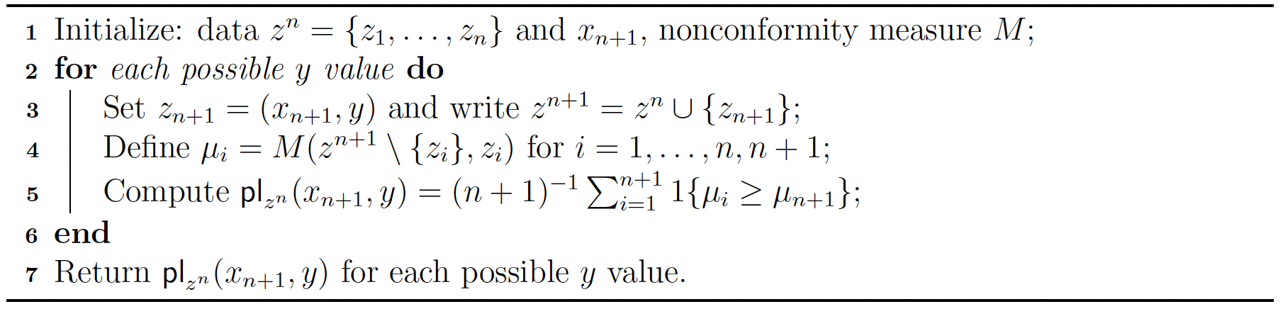
Conformal prediction starts with a deterministic mapping $M(B, z)$ of two arguments, where the first argument $B$ is a bag, i.e., a collection, of observed data, and the second argument $y$ is a provisional value of a future observation to be predicted based on the data in $B$. $M(B, z)$ measures the degree of nonconformity of the provisional value $z$ with the data in $B$. That is, when the provisional value $z$ is square with the data in $B$, $M(B, z)$ will be relatively small; otherwise, it will be relatively large. Therefore, we call $M(B, z)$ a nonconformity measure. For example, if $z$ is real-valued and $B=\{z_1, \ldots, z_n\}$, then we can take $M(B, z)=|\hat{m}_B(x)-z|$, where $\hat m_B(\cdot)$ of the conditional mean function, $\mathsf{E}(Y \mid X=\cdot)$, based on the bag $B$. The choice of nonconformity measure is not unique and is at the discretion of the actuary—in general, according to the problem at hand. Once a nonconformity measure is specified, the actuary implements the conformal prediction algorithm—Algorithm 1— to predict the value of the next label $Y_{n+1}$ at a randomly sampled feature $X_{n+1}$.

Algorithm 1.Conformal prediction (supervised learning)

In Algorithm 1, $1_A$ denotes the indicator function of an event $A$. The quantity $\mu_i(x)$, called the $i$-th nonconformity score, assigns a numerical value to $z_i$ to show how much $z_i$ agrees with the data in the augmented bag $B=z^n\cup\{z_{n+1}\}\backslash\{z_i\}$, where $z_i$ itself is excluded to avoid biases as in leave-one-out cross-validation. The function $\mathsf{pl}_{z^n}(z)$, termed the plausibility function, summarizes these nonconformity scores and outputs a value between $0$ and $1$ to indicate how plausible $z$ is as a value of $Z_{n+1}$ based on the available data $Z^n=z^n$. Based on the plausibility function output, the actuary can construct a $100(1-\alpha)\%$ conformal prediction band

$$C_\alpha(x; Z^n) = \{y: \mathsf{pl}_{Z^n}(x, y) > \alpha\},\tag{1}$$

where $\alpha\in (0, 1)$. Moreover, we have the following theorem:

Theorem 1. If $\mathsf{P}$ denotes the distribution of an exchangeable sequence $Z_1,Z_2,\ldots$, then write $\mathsf{P}^{n+1}$ for the corresponding joint distribution of $Z^{n+1}=\{Z_1,\ldots,Z_n,Z_{n+1}\}$. For $\alpha \in (0,1)$, define $t_n(\alpha) = (n+1)^{-1}\lfloor (n+1)\alpha \rfloor$, where $\lfloor a \rfloor$ denotes the greatest integer less than or equal to $a$. Then

$$\begin{align} &\sup \mathrm{P}^{n+1}\left\{\operatorname{pl}_{Z^n}\left(Z_{n+1}\right) \leq t_n(\alpha)\right\} \\&\quad\leq \alpha \quad \text { for all } n \text { and all } \alpha \in(0,1),\tag{2} \end{align}$$

where the supremum is over all distributions $\mathsf{P}$ for the exchangeable sequence.

Proof. The proof is similar to that of Theorem 1 in Hong and Martin (2021). Since $Z_1,Z_2,\ldots$ are exchangeable, we know $\mu_1,\ldots,\mu_n, \mu_{n+1}$, as functions of $(Z^n,Z_{n+1})$, are exchangeable, too. Therefore, the rank of $\mu_{n+1}$ is uniformly distributed on the set $\{1,\ldots,n,n+1\}$. By its definition, the plausibility function $\mathsf{pl}_{Z^n}(Z_{n+1})$ is proportional to the rank of $\mu_{n+1}$. Therefore, $\mathsf{pl}_{Z^n}(Z_{n+1})$ follows the discrete uniform distribution on the set $\{1/(n+1), 2/(n+1), \ldots, 1\}$. For a given $0$ < $\alpha$ < $1$, if $(n+1)\alpha$ is an integer, then $\mathsf{P}^{n+1}\{\mathsf{pl}_{n+1}(Z_{n+1})\leq t_n(\alpha) \}=\alpha$. Otherwise, we will have $\mathsf{P}^{n+1}\{ \mathsf{pl}_{n+1}(Z_{n+1})\leq t_n(\alpha) \} \leq t_n(\alpha)< \alpha$. Therefore, (2) always holds.

It follows immediately from Theorem 1 that the prediction band given by (1) is jointly valid in the sense that

$$\begin{align} &\mathsf{P}^{n+1}\{Y_{n+1}\in C_{\alpha}(X_{n+1}; Z^n) \}\\&\quad\geq 1-\alpha\quad \text{for all $(n, \mathsf{P})$},\tag{3} \end{align}$$

where $\mathsf{P}^{n+1}$ is the joint distribution for $(X_1, Y_1), \ldots, (X_n, Y_n), (X_{n+1}, Y_{n+1})$. That is, the coverage probability of prediction using the $100(1-\alpha)\%$ conformal prediction band $C_{\alpha}(x, Z^n)$ is at least $1-\alpha$ for all sample size $n$ and all distribution $\mathsf{P}$. This coverage probability result is joint, and its associated joint validity of the prediction band is different from a more desirable conditional validity property, namely,

$$\begin{align} &\mathrm{P}^{n+1}\left\{Y_{n+1} \in C_\alpha\left(X_{n+1} ; Z^n\right) \mid X_{n+1}=x\right\} \\&\quad\geq 1-\alpha \quad \text { for all }(n, \mathrm{P}) \text { and almost all } x . \end{align}$$

Conditional validity implies joint validity because

$$\begin{align} &\mathsf{P}^{n+1}\{Y_{n+1}\in C_{\alpha}(X_{n+1}; Z^n) \}\\&\quad=\mathsf{E}\left[ \mathsf{P}^{n+1}\{Y_{n+1}\in C_{\alpha}(X_{n+1}; Z^n)\mid X_{n+1}\} \right],\tag{4} \end{align}$$

where the expectation is taken with respect to the distribution of $X_{n+1}$. Conditional validity says that the probability of accurate prediction is at least $1-\alpha$ for each prediction. However, joint validity means that the rate of accurate prediction is at least $1-\alpha$, i.e., if the insurer performs an infinite sequence of independent predictions, then at least $(1-\alpha)\%$ of them are accurate. Clearly, conditional validity should be an ideal property for any fraud-detecting method. But Vovk (2012) and Lei and Wasserman (2014) show that it is impossible to achieve conditional validity property with a bounded prediction region $C_{\alpha}(X_{n+1}; Z^n)$ in supervised learning; see also Foygel-Barber et al. (2021) and Guan (2019). Hong (2023) establishes a similar result for unsupervised learning. Therefore, no practically useful fraud-detecting method can ever achieve conditional validity. It suggests that finite-sample joint validity guaranteed by conformal prediction is the best we can do. Though joint validity is a nice theoretical property, its practical meaning needs to be interpreted carefully. Note that the strong law of large numbers implies (4) can be written as

$$\begin{align} &\mathsf{P}^{n+1}\{Y_{n+1}\in C_{\alpha}(X_{n+1}; Z^n) \}\\&\quad=\lim_{m\rightarrow \infty} \frac{\sum_{i=1}^m\mathsf{P}^{n+1}\{Y_{n+1}\in C_{\alpha}(W_i; Z^n)\mid W_i\}} {m},\tag{5} \end{align}$$

where $W_1, W_2, \ldots$ is a sequence of independent random variables that have the same distribution as $X_{n+1}$. Since no insurer can conduct infinitely many predictions, this means that if the insurer performs a sufficiently large number of independent predictions, then about $(1-\alpha)\%$ of them will be accurate, because the right-hand side of (5) may or may not have converged for finitely many predictions. Also, this interpretation does not contradict the finite-sample validity of the $100(1-\alpha)\%$ conformal prediction band. The latter refers to the fact that the inequality in (3) holds for any finite sample $(X_1, Y_1), \ldots, (X_n, Y_n)$. Furthermore, for two different coverage probability levels $\alpha_1$ and $\alpha_2$, the corresponding conformal prediction regions $C_{\alpha_1}(X_{n+1}; Z^n)$ and $C_{\alpha_2}(X_{n+1}; Z^n)$ are different. Therefore, convergence in (5) depends not only on the training data but also on $\alpha$. Finally, finite-sample validity, given by (3), is not to be confused with finite-sample generalization error bound: the former does not depend on any loss function, while the latter depends on the choice of a loss function.

It bears noting that conformal prediction has three potential drawbacks: (1) one may not be able to implement Algorithm 1 for all possible $y$, jeopardizing finite-sample validity; (2) the shape of the conformal prediction region $C_{\alpha_1}(X_{n+1}; Z^n)$ could be irregular, rendering it useless in practice; and (3) the computation required for implementing Algorithm 1 could be prohibitively expensive. In a regression problem, (1) and (3) are major concerns for conformal prediction. Fortunately, we do not need to worry about them for the problem of detecting insurance fraud, because there are only two possible values of $y$ and the resulting conformal prediction region can only take four possible shapes; see the next section for details. However, (2) is a challenge we must overcome in applying conformal prediction to insurance fraud detection. To circumvent this difficulty, we will propose a nonconformity measure and derive close-form formulas for the resulting conformal prediction region.

3. Proposed method

In this article, we consider two cases: (1) all features are continuous and (2) all features are categorical. It is evident that the aforementioned conformal prediction band $C_{\alpha}(Z^n)$ depends on the choice of the nonconformity measure $M$. Therefore, the proposed nonconformity measures are different for these two cases. The choice of the nonconformity measure is not unique. In practice, the actuary may choose other appropriate nonconformity measures.

3.1. Continuous features

Suppose $Z_1, ... , Z_n$ are observed data where $Z_i=(X_i, Y_i)$, $X_i \in \mathbb{R}^p$, $p \geq 2$, and $Y_i \in \{0,1\}$. Define a bag of data $B\equiv Z^{n}$ where $Z^{n}=\{Z_1, ..., Z_n\}$. For the $(n+1)$-th observation, $Z_{n+1}=(X_{n+1}, Y_{n+1})$, $X_{n+1}$ is known. The goal is to determine $Y_{n+1}$ based on $X_{n+1}$ and the data in the bag $B$. Without loss of generality, we may assume $Y_i=0$ for $1\leq i\leq m$ and $Y_i=1$ for $m+1\leq i\leq n$ for some integer $1\leq m\leq n$.

The nonconformity measure we choose here is

$$M(B, z)=\bigg| \bigg| \overline{X}_{B\cup \{(x, y)\},y}-x \bigg| \bigg|,$$

where $z=(x, y)$, $||\cdot||$ is the Euclidean norm on $\mathbb{R}^p$, and $\overline{X}_{B\cup \{(x, y)\},y}$ denotes the vector obtained by averaging all the $X_i$s whose labels $Y_{i}=y$ in the bag $B\cup \{(x, y)\}$. For example, if $p=1$, $B=\{(1, 0), (8, 1), (5, 0)\}$, and $z=(3, y)$ where $y\in \{0, 1\}$, then

$$\begin{align} M(B, z)&=| \overline{X}_{B\cup \{(x, y)\}, y}-x|\\&=\left\{ \begin{array}{ll} |(1+5)/2-3|=0, & \hbox{if $y=0$;} \\ &\\ |8-3|=5, & \hbox{if $y=1$.} \end{array} \right. \end{align}$$

Since all norms are equivalent on a finite-dimensional Euclidean space, our choice of the Euclidean norm is made without loss of generality.

To derive the $100(1-\alpha)\%$ conformal prediction band $C_{\alpha}(x; Z^n)$, we need to consider two cases: (I) $Y_{n+1}=0$ and (II) $Y_{n+1}=1$.

Case I: $Y_{n+1}=0$. The $i$-th nonconformity score is given by

$$\small{ \begin{split} \mu_i&=M(Z^{n+1}\backslash\{Z_i\}, Z_i)\\ &=\left\{ \begin{array}{lr} \bigg | \bigg |\overline{X}_{(Z^{n+1}\backslash\{Z_i\}) \cup \{Z_i\}, 0}-X_i \bigg | \bigg |, \text{ if } Y_i=0; &\\ &\\ \bigg | \bigg |\overline{X}_{(Z^{n+1}\backslash\{Z_i\}) \cup \{Z_i\}, 1}-X_i \bigg | \bigg |, \text{ if } Y_i=1. \end{array} \right.\\ &=\left\{ \begin{array}{lr} \left((\overline{X}_{Z^{n+1}, 0}-X_i)^\mathbb{T}(\overline{X}_{Z^{n+1}, 0}-X_i)\right)^{1/2}, \text{ if } Y_i=0; &\\ \left((\overline{X}_{Z^{n+1}, 1}-X_i)^\mathbb{T}(\overline{X}_{Z^{n+1}, 1}-X_i) \right)^{1/2}, \text{ if } Y_i=1. \end{array} \right. \\ \mu_{n+1}&=\bigg | \bigg |\overline{X}_{Z^{n+1}, 0}-X_{n+1}\bigg | \bigg |\\ &=((\overline{X}_{Z^{n+1}, 0}-X_{n+1})^\mathbb{T}(\overline{X}_{Z^{n+1}, 0}-X_{n+1}))^{1/2}, \end{split}}$$

where the superscript $\mathbb{T}$ used in the last equality denotes matrix transpose. When $Y_i=0$, we can rewrite $\mu_i \geq \mu_{n+1}$ as:

$$\scriptsize{ \begin{align} \begin{split} \mu_i \geq \mu_{n+1} & \Leftrightarrow \left((\overline{X}_{Z^{n+1}, 0}-X_i)^\mathbb{T}(\overline{X}_{Z^{n+1}, 0}-X_i) \right)^{1/2} \\&\quad\geq \left( (\overline{X}_{Z^{n+1}, 0}-X_{n+1})^\mathbb{T}(\overline{X}_{Z^{n+1}, 0}-X_{n+1}) \right)^{1/2}\\ & \Leftrightarrow (\overline{X}_{Z^{n+1}, 0}-X_i)^\mathbb{T}(\overline{X}_{Z^{n+1}, 0}-X_i) \\&\quad\geq (\overline{X}_{Z^{n+1}, 0}-X_{n+1})^\mathbb{T}(\overline{X}_{Z^{n+1}, 0}-X_{n+1})\\ &\Leftrightarrow X_i^\mathbb{T} X_i-2X_i^\mathbb{T}\overline{X}_{Z^{n+1}, 0}+\overline{X}_{Z^{n+1}, 0}^{\mathbb{T}} \overline{X}_{Z^{n+1}, 0} \\&\quad\geq X_{n+1}^\mathbb{T} X_{n+1}-2 X_{n+1}^\mathbb{T} \overline{X}_{Z^{n+1}, 0}+ \overline{X}_{Z^{n+1}, 0}^{\mathbb{T}} \overline{X}_{Z^{n+1}, 0}\\ & \Leftrightarrow X_{n+1}^\mathbb{T} X_{n+1}- X_i^\mathbb{T} X_i -2 X_{n+1}^\mathbb{T} \overline{X}_{Z^{n+1}, 0}\\&\quad+2X_i^\mathbb{T}\overline{X}_{Z^{n+1}, 0} \leq 0\\ &\Leftrightarrow (X_{n+1}-X_i)^\mathbb{T} (X_{n+1}+X_i)\\&\quad-2(X_{n+1}-X_i)^\mathbb{T} \overline{X}_{Z^{n+1}, 0} \leq 0\\ & \Leftrightarrow (X_{n+1}-X_i)^\mathbb{T} (X_{n+1}+X_i)\\&\quad-2(X_{n+1}-X_i)^\mathbb{T}\frac{\sum_{k=1}^{m} X_k+X_{n+1} }{m+1} \leq 0\\ &\qquad \quad \Leftrightarrow (X_{n+1}-X_i)^\mathbb{T} \left(X_{n+1}+X_i-2\frac{\sum_{k=1}^{m} X_k+X_{n+1} }{m+1}\right) \leq 0\\ &\qquad \quad \Leftrightarrow (X_{n+1}-X_i)^\mathbb{T}\left(\frac{m-1}{m+1}X_{n+1}+X_i-2\frac{\sum_{k=1}^{m} X_k}{m+1}\right) \leq 0 \\ &\qquad \quad \Leftrightarrow (X_{n+1}-X_i)^\mathbb{T}\left[X_{n+1}-\left(2\frac{\sum_{k=1}^{m} X_k}{m-1}-\frac{m+1}{m-1}X_i\right)\right] \leq 0. \end{split} \end{align}}$$

When $Y_i=1$, we can rewrite $\mu_i \geq \mu_{n+1}$ as:

$$\small{ \begin{split} \mu_i \geq \mu_{n+1} &\Leftrightarrow \bigg | \bigg |\overline{X}_{Z^{n+1},1}-X_i \bigg| \bigg| \geq \bigg| \bigg |\overline{X}_{Z^{n+1},0}-X_{n+1} \bigg| \bigg|\\ &\Leftrightarrow \bigg | \bigg |\frac{\sum_{k=m+1}^{n} X_k}{n-m}-X_i \bigg | \bigg | \geq\bigg | \bigg |\frac{\sum_{k=1}^{m}X_k+X_{n+1}}{m+1}-X_{n+1} \bigg | \bigg |\\ &\Leftrightarrow \bigg | \bigg |\frac{\sum_{k=m+1}^{n} X_k}{n-m}-X_i \bigg | \bigg|^2 \geq \bigg | \bigg |\frac{\sum_{k=1}^{m}X_k}{m+1}-\frac{m}{m+1}X_{n+1} \bigg | \bigg|^2\\ &\Leftrightarrow \bigg | \bigg|\frac{\sum_{k=1}^{m}X_k}{m+1}-\frac{m}{m+1}X_{n+1} \bigg | \bigg |^2-\bigg | \bigg|\frac{\sum_{k=m+1}^{n} X_k}{n-m}-X_i \bigg | \bigg|^2 \leq 0\\ &\Leftrightarrow \left( \bigg | \bigg |\frac{m}{m+1}X_{n+1}-\frac{\sum_{k=1}^{m}X_k}{m+1} \bigg | \bigg |+ \bigg| \bigg |\frac{\sum_{k=m+1}^{n} X_k}{n-m}-X_i \bigg | \bigg| \right)\\ & \left( \bigg | \bigg|\frac{m}{m+1}X_{n+1}-\frac{\sum_{k=1}^{m}X_k}{m+1} \bigg | \bigg |-\bigg | \bigg|\frac{\sum_{k=m+1}^{n} X_k}{n-m}-X_i \bigg | \bigg |\right) \leq 0. \end{split}}$$

Therefore, the plausibility value $\mathsf{pl}_{Z^{n}}(Y_{n+1}=0, X_{n+1})$ is given by

$$\scriptsize{ \begin{aligned} &\mathrm{pl}_{Z^n}\left(Y_{n+1}=0, X_{n+1}\right) \\& =\frac{1}{n+1} \sum_{i=1}^{n+1} \mathbb{I}\left(\mu_i \geq \mu_{n+1}\right) \\ & =\frac{1}{n+1} \sum_{i=1}^{n+1}\left\{\mathbb{I}\left\{\left(X_{n+1}-X_i\right)^{\mathbb{T}}\left[X_{n+1}-\left(2 \frac{\sum_{k=1}^m X_k}{m-1}-\frac{m+1}{m-1} X_i\right)\right] \leq 0\right\}\right. \\ & +\mathbb{I}\left\{\left(\left\|\frac{m}{m+1} X_{n+1}-\frac{\sum_{k=1}^m X_k}{m+1}\right\|+\left\|\frac{\sum_{k=m+1}^n X_k}{n-m}-X_i\right\|\right)\right. \\ & \left.\left.\left.\left(\left\|\frac{m}{m+1} X_{n+1}-\frac{\sum_{k=1}^m X_k}{m+1}\right\|-\left\|\frac{\sum_{k=m+1}^n X_k}{n-m}-X_i\right\|\right) \leq 0\right)\right\}\right\} . \end{aligned} \tag{6}}$$

Case II: $Y_{n+1}=1$. As in the case where $Y_{n+1}=0$, we can derive that

$$\small{ \begin{split} \mu_i&=M(Z^{n+1}\backslash\{Z_i\}, Z_i)\\ &=\left\{ \begin{array}{lr} \bigg | \bigg |\overline{X}_{Z^{n+1}, 0}-X_i \bigg | \bigg |, \text{ if } Y_i=0; &\\ &\\ \bigg | \bigg |\overline{X}_{Z^{n+1}, 1}-X_i \bigg | \bigg |, \text{ if } Y_i=1. \end{array} \right. \\ &=\left\{ \begin{array}{lr} ((\overline{X}_{Z^{n+1}, 0}-X_i)^\mathbb{T}(\overline{X}_{Z^{n+1}, 0}-X_i))^{1/2}, \text{ if } Y_i=0; &\\ ((\overline{X}_{Z^{n+1}, 1}-X_i)^\mathbb{T}(\overline{X}_{Z^{n+1}, 1}-X_i))^{1/2}, \text{ if } Y_i=1. \end{array} \right. \\ \mu_{n+1}&=\bigg | \bigg |\overline{X}_{Z^{n+1}/\{Z_i\}, 1}-X_{n+1}\bigg | \bigg |\\ &=((\overline{X}_{Z^{n+1}, 1}-X_{n+1})^\mathbb{T}(\overline{X}_{Z^{n+1}, 1}-X_{n+1}))^{1/2}. \end{split}}$$

When $Y_i=0$, we can rewrite $\mu_i \geq \mu_{n+1}$ as

$$\scriptsize{ \begin{align} \mu_i \geq \mu_{n+1} &\Leftrightarrow \bigg | \bigg |\overline{X}_{Z^{n+1},0}-X_i\bigg | \bigg | \geq \bigg | \bigg |\overline{X}_{Z^{n+1},1}-X_{n+1}\bigg | \bigg |\\ &\Leftrightarrow \bigg | \bigg |\frac{\sum_{k=1}^{m} X_k}{m}-X_i \bigg | \bigg | \geq \bigg | \bigg |\frac{\sum_{k=m+1}^{n}X_k+X_{n+1}}{n-m+1}-X_{n+1}\bigg | \bigg |\\ &\Leftrightarrow \bigg | \bigg |\frac{\sum_{k=1}^{m} X_k}{m}-X_i \bigg | \bigg |^2 \geq \bigg | \bigg |\frac{\sum_{k=m+1}^{n}X_k}{n-m+1}-\frac{n-m}{n-m+1}X_{n+1}\bigg | \bigg |^2\\ &\Leftrightarrow \bigg | \bigg |\frac{n-m}{n-m+1}X_{n+1}-\frac{\sum_{k=m+1}^{n}X_k}{n-m+1}\bigg | \bigg |^2-\bigg | \bigg |\frac{\sum_{k=1}^{m} X_k}{m}-X_i \bigg | \bigg |^2 \leq 0\\ &\Leftrightarrow \left( \bigg | \bigg |\frac{n-m}{n-m+1}X_{n+1}-\frac{\sum_{k=m+1}^{n}X_k}{n-m+1}\bigg | \bigg |+\bigg | \bigg |\frac{\sum_{k=1}^{m} X_k}{m}-X_i \bigg | \bigg | \right)\\ &\left( \bigg | \bigg |\frac{n-m}{n-m+1}X_{n+1}-\frac{\sum_{k=m+1}^{n}X_k}{n-m+1}\bigg | \bigg |-\bigg | \bigg |\frac{\sum_{k=1}^{m} X_k}{m}-X_i \bigg | \bigg |\right) \leq 0. \end{align}}$$

When $Y_i=1$, we can rewrite $\mu_i \geq \mu_{n+1}$ as

$$\scriptsize{ \begin{align} \mu_i \geq \mu_{n+1} & \Leftrightarrow ((\overline{X}_{Z^{n+1}, 1}-X_i)^\mathbb{T}(\overline{X}_{Z^{n+1}, 1}-X_i))^{1/2} \\&\quad\geq ((\overline{X}_{Z^{n+1}, 1}-X_{n+1})^\mathbb{T}(\overline{X}_{Z^{n+1}, 1}-X_{n+1}))^{1/2}\\ &\Leftrightarrow (\overline{X}_{Z^{n+1}, 1}-X_i)^\mathbb{T}(\overline{X}_{Z^{n+1}, 1}-X_i) \\&\quad\geq(\overline{X}_{Z^{n+1}, 1}-X_{n+1})^\mathbb{T}(\overline{X}_{Z^{n+1}, 1}-X_{n+1})\\ &\Leftrightarrow X_{n+1}^\mathbb{T} X_{n+1}-2 X_{n+1}^\mathbb{T} \overline{X}_{Z^{n+1}, 1}\\&\quad- X_i^\mathbb{T} X_i+2X_i^\mathbb{T}\overline{X}_{Z^{n+1}, 1} \leq 0\\ &\Leftrightarrow (X_{n+1}-X_i)^\mathbb{T}(X_{n+1}+X_i)\\&\quad-2(X_{n+1}-X_i)^\mathbb{T}\overline{X}_{Z^{n+1},1}\leq 0\\ &\Leftrightarrow (X_{n+1}-X_i)^\mathbb{T}(X_{n+1}+X_i-2\overline{X}_{Z^{n+1},1})\leq 0\\ &\qquad \Leftrightarrow (X_{n+1}-X_i)^\mathbb{T}(X_{n+1}+X_i-2\frac{\sum_{k=m+1}^{n} X_k+X_{n+1}}{n-m+1}) \leq 0\\ &\qquad \Leftrightarrow (X_{n+1}-X_i)^\mathbb{T}(\frac{n-m-1}{n-m+1}X_{n+1}+X_i-2\frac{\sum_{k=m+1}^{n} X_k}{n-m+1}) \leq 0\\ &\qquad \Leftrightarrow (X_{n+1}-X_i)^\mathbb{T}\left[X_{n+1}-\left(2\frac{\sum_{k=m+1}^{n}X_k}{n-m-1}-\frac{n-m+1}{n-m-1}X_i \right)\right] \leq 0. \end{align}}$$

It follows that the plausibility value $\mathsf{pl}_{Z^{n}}(Y_{n+1}=1, X_{n+1})$ is given by

$$\tiny{ \begin{align} &\mathsf{pl}_{Z^{n}}(Y_{n+1}=1, X_{n+1})\\&=\frac{1}{n+1}\sum_{i=1}^{n+1}\mathbb{I}(\mu_i\geq\mu_{n+1})\\ &=\frac{1}{n+1} \sum_{i=1}^{n+1} \left\{\mathbb{I}\left\{ \left( \bigg | \bigg |\frac{n-m}{n-m+1}X_{n+1}-\frac{\sum_{k=m+1}^{n}X_k}{n-m+1}\bigg | \bigg |+\bigg | \bigg |\frac{\sum_{k=1}^{m} X_k}{m}-X_i \bigg | \bigg |\right)\right. \right.\\ &\left. \left( \bigg | \bigg |\frac{n-m}{n-m+1}X_{n+1}-\frac{\sum_{k=m+1}^{n}X_k}{n-m+1}\bigg | \bigg |-\bigg | \bigg |\frac{\sum_{k=1}^{m} X_k}{m}-X_i \bigg | \bigg |\right) \leq 0\right\}\\ &+\mathbb{I}\left. \left\{(X_{n+1}-X_i)^\mathbb{T}\left[X_{n+1}-\left(2\frac{\sum_{k=m+1}^{n}X_k}{n-m-1}-\frac{n-m+1}{n-m-1}X_i \right)\right] \leq 0\right\} \right\}. \end{align} \tag{7}}$$

Thus, the $100(1-\alpha)\%$ conformal prediction band given by

$$\tiny{ \begin{align} &C_\alpha(X_{n+1}, Z^n)\\&=\left\{ \begin{array}{lr} \{0\},\ \ \text{if}\ \ \mathsf{pl}_{Z^{n}}(Y_{n+1}=0, X_{n+1})> \alpha \ \ \text{and} \ \ \mathsf{pl}_{Z^{n}}(Y_{n+1}=1, X_{n+1})\leq \alpha; \\ \{1\}, \ \ \text{if}\ \ \mathsf{pl}_{Z^{n}}(Y_{n+1}=0, X_{n+1})\leq \alpha \ \ \text{and} \ \ \mathsf{pl}_{Z^{n}}(Y_{n+1}=1, X_{n+1}) > \alpha; \\ \{0,1\}, \ \ \text{if both}\ \ \mathsf{pl}_{Z^{n}}(Y_{n+1}=0, X_{n+1})> \alpha \ \ \text{and} \ \ \mathsf{pl}_{Z^{n}}(Y_{n+1}=1, X_{n+1})> \alpha; \\ \emptyset,\ \ \text{if}\ \ \mathsf{pl}_{Z^{n}}(Y_{n+1}=0, X_{n+1})\leq \alpha \ \ \text{and} \ \ \mathsf{pl}_{Z^{n}}(Y_{n+1}=1, X_{n+1})\leq \alpha,\\ \end{array} \right.\end{align}\tag{8}}$$

where $\mathsf{pl}_{Z^{n}}(Y_{n+1}=0, X_{n+1})$ and $\mathsf{pl}_{Z^{n}}(Y_{n+1}=1, X_{n+1})$ are calculated using (6) and (7).

A few remarks are in order. The first two cases in (8) where $C_\alpha(X_{n+1}, Z^n)=\{0\}$ and $C_\alpha(X_{n+1}, Z^n)=\{1\}$ denote the classification results of a valid claim and a fraudulent claim, respectively. When $C_\alpha(X_{n+1}, Z^n)=\{0, 1\}$, the conformal prediction classifier says the claim at hand is either a valid claim or a fraudulent claim, which is always true and not helpful for practitioners. Such a result will be deemed “noninformative.” If $C_\alpha(X_{n+1}, Z^n)$ turns out to be the empty set, then the conformal prediction classifier cannot generate any $100(1-\alpha)\%$ conformal prediction band based on given data. This means the coverage probability level $(1-\alpha)\%$ is too high for a given information $Z_1, \dots, Z_n$. In practice, a claim that results in $C_\alpha(X_{n+1}, Z^n)=\{1\}$ will automatically be flagged for further investigation according to the insurance fraud detecting process described in Section 1. In addition, any claim leading to $C_\alpha(X_{n+1}, Z^n)=\{0, 1\}$ and $C_\alpha(X_{n+1}, Z^n)=\emptyset$ should be further examined by other classification methods or investigated by the fraud-detecting staff of the insurer.

3.2. Categorical features

To consider the case where features are categorical, we let $Z_1, ... , Z_n$ be observed data for fraud detection, where $Z_i=(X_i, Y_i)$, $X_i =(X_{i1}, ... , X_{ip})$ and $X_{ij} \in \{c_{j1},...,c_{j{m_j}}\}$ is categorical, and $Y_i \in \{0,1\}$. Define a bag of data $B \equiv Z^n$, where $Z^n=\{Z_1,...,Z_n\}$. For the $(n+1)$-th observation, $Z_{n+1}=(X_{n+1}, Y_{n+1})$, where $X_{n+1}$ is known. As in the case of continuous features, our task here is to predict the value of $Y_{n+1}$ given $X_{n+1}$ based on the bag $B=\{Z_1, \ldots, Z_n\}$. To this end, we will first transfer all categorical features to numerical values using frequency encoding. That is, for each categorical value a feature takes, we replace it with the frequency of the occurrence of that category in that data. That is, for $j=1, \ldots, p$ and $k=1, \ldots, m_j$ we replace the value $c_{jk}$ in the original data with the new value $\frac{\sum_{i=1}^n \mathbb{I}(X_{ij}=c_{jk})}{\sum_{k=m_j}^p\sum_{i=1}^n \mathbb{I}(X_{ij}=c_{jk})}$. Once we finish this frequency encoding, we apply our conformal prediction classifier to the encoded data. Though frequency encoding converts the features to numbers, it does not change the categorical nature of these features, and the resulting features still take only finitely many values in $[0, 1]$. Therefore, fraud detection is expected to be more challenging here than in the above case of continuous features; see Section 4.2 for a concrete example.

4. Examples

4.1. Continuous features

Example 1. The data used in this example are the same as the data $\mathcal{D}_2$ in Gomes, Jin, and Yang (2021). They consist of credit card transactions made by European cardholders in September 2013. The dataset is available at https://www.kaggle.com/datasets/mlg-ulb/creditcardfraud. It was collected during a research collaboration of Worldline and the Machine Learning Group (http://mlg.ulb.ac.be) of ULB (Université Libre de Bruxelles) on big data mining and fraud detection. In total, there are 284,807 transactions; 492 of them are fraudulent. The raw data have been anonymized for confidentiality. The resulting dataset contains 30 continuous features and one categorical label (i.e., the fraud indicator). The label is tagged as “class”; it takes the value $1$ if the claim is fraudulent and $0$ otherwise. Of the 30 features, 28 (labeled as V1 to V28) are the principal analysis components obtained from the raw data, and the remaining two, labeled “time” and “amount” respectively, are the claim time and the claim amount. The features “time” and “amount” and the label “class” have not been transformed and are the same as in the raw data. This dataset is highly imbalanced: the positive class (frauds) accounts for $0.172\%$ of all transactions.

We take the validation set approach with a $75\%-25\%$ split of the original dataset into the training dataset and the test dataset. The training dataset consists of $213,228$ legitimate claims and $377$ fraudulent claims. The test dataset has $71,087$ valid claims and $115$ fraudulent claims. Here we take the first six principal components to be our features. For $\alpha=0.2, 0.15, 0.10$, and $0.05$, we train our conformal prediction classifier on the training dataset and then test it on the test dataset. Table 1 reports the results, where the test error rate is calculated as

$$\text{test error rate $=\frac{\text{FN+FP}}{\text{test data sample size}}$}.$$

Here “noninformative” corresponds to the case where the prediction band $C_{\alpha_1}(X_{n+1}; Z^n)$ is $\{0, 1\}$. That is, the conformal prediction classifier can only tell the user that a claim must be either valid or fraudulent, which is not informative. Alternatively, “empty” is the case where $C_{\alpha_1}(X_{n+1}; Z^n)=\emptyset$. This means that the conformal prediction classifier is unable to tell whether a claim is either valid or fraudulent. Neither case is useful.

For each chosen value of $\alpha$, the false positive counts are more than the false negative counts, but the test error rate is below the coverage probability level $\alpha$. As we mentioned in Section 2, we must exercise caution in interpreting the numeral results produced by conformal prediction. Although the $100(1-\alpha)\%$ prediction band $C_{\alpha_1}(X_{n+1}; Z^n)$ is provably valid, the test error rate in any real-world example may or may not be less than $\alpha$ because we can only test our conformal prediction classifier a finite number of times in a real-world example, and there is no way to guarantee that convergence in (5) has been achieved in such a case. In this example, we are confident that the convergence has been achieved. In addition, any statistics-based or data science–based fraud-detecting tool only serves as an initial screening tool in practice. For this reason, a test error rate of $20\%$ is already considered to be very good. Moreover, for $\alpha$ values of $20\%$, $15\%$, $10\%$, and $5\%$, our conformal prediction classifier is able to label a claim in the test dataset as fraudulent or valid $83\%$, $86\%$, $90\%$, and $93\%$ of the time, respectively. Given these observations, the performance of our method is excellent.

It is customary to compare a new method to some existing methods. However, we are not aware of any existing methods in the insurance literature that can provide finite-sample validity. Therefore, we compare the performance of our method with the two latest methods along these lines. The two methods, proposed by Gomes, Jin, and Yang (2021), are (a) variational autoencoder (VAE) and (b) autoencoder (AE). We will take (a) as the baseline model. Table 2 summarizes the results. Note that AE and VAE both have a parameter called the reconstruction error threshold (RE-T), but neither provides information about possible noninformative or empty cases. Also, the preassigned coverage probability level $\alpha$ does not apply to AE or VAE. However, TP, FN, FP, TN, and test error rate apply to all fraud-detecting methods. The second column of Table 2 refers to the $\alpha$ level for the conformal prediction region or the tuning parameter RE-T of VAE and AE. RE-T is a tuning parameter, but $\alpha$ is not. Therefore, one must exercise caution in interpreting Table 2. In particular, an RE-T value of 40 for VAE or AE is not comparable to an $\alpha$ value of $5\%$ for conformal prediction.

Table 2 shows that both VAE and VE perform better as RE-T increases. Specifically, TP and TN increase as RE-T increases, while FN, FP, and test error rate decrease as RE-T decreases. Regarding TP, FN, FP, and TN, conformal prediction seems to be relatively conservative compared to VAE and AE. This does not mean VAE or AE is better than conformal prediction. First, neither VAE nor AE guarantees finite-sample validity, while conformal prediction achieves validity at every chosen $\alpha$ level, which is the key strength of the proposed method. Second, there is no established relationship between RE-T and test error rate. In particular, the choice of RE-T is subjective, and the actuary cannot know the exact RE-T value for achieving a test error rate below a given $\alpha$ level. Third, the fraud data is highly imbalanced: its entries are dominantly nonfraudulent. Hence, when the actuary raises the RE-T level of VAE or AE, TN will increase and FP will decrease. This will generally reduce the test error rate. Therefore, it is difficult to distinguish this general effect from the performance of VAE and AE in any empirical study. In sum, VAE or AE might perform better than the proposed method in some cases, but this possibility does not provide any useful information for our purpose: to design an automated fraud-detecting method that is used for initial screening. In particular, given an $\alpha$ value, an actuary cannot know beforehand what value of RE-T is needed for an automated fraud-detecting method based on VAE or AE to perform better than conformal prediction. Even so, the proposed method tends to be conservative, but it has been proven to guarantee finite-sample validity.

Example 2. The insurance fraud dataset used in this example consists of insurance claims provided by a major insurer in Spain from 2015–2016. Like the credit card fraud data in the previous example, the dataset has been anonymized due to its confidential nature. The dataset is available at https://data.mendeley.com/datasets/g3vxppc8k4/2. It contains a total of 163,182 claims, of which 13,037 are fraudulent. There are 325 continuous features labeled from $0$ to $324$, one categorical feature, and one categorical label. The categorical feature represents the claim ID, and the categorical label, which only takes values in the set $\{0, 1\}$, is the fraud indicator. It is unclear from the data what the continuous features stand for. However, this does not affect the applicability of our method. To make the data manageable to analyze, we apply the principal component analysis transformation across all features except the categorical feature. Then we select the first six principal components as the features for our conformal prediction classifier. As in the previous example, we take the validation set approach and split the data into a training dataset ($75\%$ or 122,387 claims) and a test dataset ($25\%$ or 40,795 claims). In the training dataset, there are $112,640$ valid claims and $9,746$ fraudulent claims. The test dataset has $37,505$ valid claims and $3,291$ fraudulent claims. For $\alpha=0.2, 0.15, 0.10$, and $0.05$, we train our conformal prediction classifier on the training set and then test it on the test dataset. Table 3 summarizes the key quantities from the results. As in the previous examples, the test error rate is below the coverage probability level $\alpha$ across four different values of $\alpha$. This again demonstrates the excellent performance of our conformal prediction classifier.

Finally, we point out that no fraud-detecting method, including our conformal prediction classifier, will work well if the given data are not informative enough in the sense that the correlation coefficient between each feature and the label is very low. This is not a drawback of our method. When all features are barely correlated with the label, the information supplied by the features has little bearing on the label. In this case, no method is expected to provide a reasonable solution. For example, the highest correlation coefficient between the six principal components and the label in Example 1 is $0.1929$. Though the correlation coefficient is a bit low, the huge sample size compensates for it, and the result is satisfying. For the Mendeley data, the highest correlation coefficient between the six principal components and the label is $0.7721$. To further illustrate this point, we consider leaving out all features except six features with the lowest absolute correlation coefficients (i.e., coefficients $-2.45\times10^{-5}$, $2.48\times10^{-5}$, $6.33\times10^{-5}$, $-8.32\times10^{-5}$, $1.07\times10^{-4}$, and $1.24\times10^{-4}$) and keeping the label. Now we apply our method to this modified dataset. Table 4 shows that the results are completely unsatisfactory.

In practice, an actuary should first check whether at least one feature is correlated with the label to a reasonable extent. In the case of continuous features, this can be done by calculating the correlation coefficient between each feature and the label. If the answer is affirmative, then the actuary can proceed further to select the right tool for fraud detection. Otherwise, the task of fraud detection may be too challenging to be completed without more data. Also, a large sample size can compensate for a relatively weak correlation.

4.2. Categorical features

Intuitively, the requirement that at least one feature is associated with the label to a reasonable extent should also apply when the features are categorical. In this case, the correlation coefficient is no longer appropriate for measuring the association between categorical variables. Instead, we should use Cramér’s V.

Let $X$ and $Y$ be two categorical variables such that $X$ takes categorical values $x_1, \ldots, x_s$ and $Y$ takes categorical values $y_1, \ldots, y_t$. For a sample of $(X, Y)$ with size $n$, we put

$$\begin{aligned} n_{i\cdot} &= \text{the number of times $x_i$ is observed in the data},\\ n_{\cdot j} &= \text{the number of times $y_j$ is observed in the data},\\ n_{ij} &= \text{the number of times $(x_i, y_j)$ is observed in the data}. \end{aligned}$$

Then the corresponding chi-squared statistic is given by

$$\chi^2=\sum_{i=1}^s \sum_{j=1}^t \frac{\left(n_{ij}-n_{i\cdot} n_{\cdot j}/n_{ij}\right)^2}{n_{i\cdot} n_{\cdot j}/n_{ij}}.$$

Cramér’s V between $X$ and $Y$, denoted as $V(X, Y)$ is defined as

$$V(X, Y)=\sqrt{\frac{\chi^2/n}{\min\{s-1, t-1\}}}.$$

Like the correlation coefficient, $V(X, Y)$ takes values in $[0, 1]$ where a higher value of $V(X, Y)$ means a higher degree of association between $X$ and $Y$ and vice versa. In particular, $0$ and $1$ denote total lack of association and perfect association, respectively.

Example 3. Here we consider a public dataset that contains auto insurance claims over a year in a given territory. The data are available from the link https://www.kaggle.com/code/buntyshah/insurance-fraud-claims-detection. There are $32$ categorical features and one categorical label that denotes whether a claim is legitimate or fraudulent. The data contain a total of $15,420$ claims. Like the previous two datasets, this auto insurance claim dataset displays a typical imbalance: $14,497$ legitimate claims and $923$ fraudulent claims.

To apply our conformal prediction classifier, we first encode all the categorical features using the frequency of observations within each category. Take the feature WitnessPresent for an example. This feature has $15, 333$ occurrences with no witness and $87$ occurrences with a witness present. Then the two categorical values “no witness” and “witness present” will be encoded as two numerical values $15,333/15,420$ and $87/15,420$, respectively. For the encoded data, we check Cramér’s V between each feature and the label. It turns out that each feature is very weakly associated with the label: the largest value of Cramér’s V is only $0.1684$. This shows that features are weakly associated with the label. Moreover, the additional challenge for the categorical feature mentioned at the end of Section 3.2 makes things even worse. Thus, our method is not expected to perform well on such a dataset. To see this, we still follow the validation set approach to make a $75\%-25\%$ split of the encoded data into a training dataset and a test dataset. The training dataset consists of $10,874$ valid claims and $691$ fraudulent claims, while the test dataset contains $3,623$ valid claims and $232$ fraudulent claims. Next, we train our conformal prediction classifier on the training dataset before testing it on the test dataset, using six features having the highest association with the label. Table 5 displays the results.

The performance of our conformal prediction classifier is unsatisfying. This public dataset is not informative enough, in the sense that the association between each feature and the label is too weak. In particular, Table 5 shows that our conformal prediction classifier discovers many noninformative cases. This is not a flaw of our method. Quite the opposite—it shows that our conformal prediction classifier can tell the actuary that the data are noninformative when they are.

Next, we use the R package “GenOrd” to simulate a new categorical variable $\widetilde{X}$ such that Cramér’s V between $\widetilde{X}$ and the label $Y$ equals 0.75. Then, we form a simulated dataset using this simulated feature, the label from the original data, and the five features with the highest value of Cramér’s V’s with the label in the original data. Finally, we apply our conformal prediction classifier on the simulated data for $\alpha=0.05, 0.10, 0.15$, and $0.20$. The results are summarized in Table 6. Since the association of $\widetilde{X}$ and $Y$ is high, the results are satisfactory, and the test error rate is lower than each chosen $\alpha$ level.

To further investigate the degree of association of the features with the label on prediction accuracy, we repeat the aforementioned simulation for $V(\widetilde{X}, Y)=0.45$ and $V(\widetilde{X}, Y)=0.15$. Tables 7 and 8 demonstrate the results. For the case where the association between $\widetilde{X}$ and $Y$ is medium, i.e., $V(\widetilde{X}, Y)=0.45$, the results are mixed. When the targeted $\alpha$ level is not too demanding, i.e., $\alpha=0.20$ and $0.15$, the test error rate is lower than $\alpha$, but for $\alpha=0.10$ and $0.05$, the test error rate is unacceptably higher than $\alpha$. When the association between $\widetilde{X}$ and $Y$ is low, i.e., $V(\widetilde{X}, Y)=0.15$, the results are unacceptable for each given $\alpha$ level. Recall that the highest value of Cramér’s V between a feature and $Y$ in the original data is $0.1684$. If $V(\widetilde{X}, Y)=0.15$, then the highest Cramér’s V between $Y$ and any of the six features in this simulated data will still be $0.1684$. Therefore, the unsatisfying performance of the conformal prediction classifier here is no surprise.

5. Concluding remarks

We have proposed a new fraud-detecting method based on a general machine learning strategy called conformal prediction. Our method has three desirable properties: (1) it guarantees finite-sample validity, (2) it is model-free, and (3) it has a solid theoretical backup. For practical purposes, when actuaries apply our method to predict possible fraudulent claims, the test error rate is expected to be below the preassigned level when at least one feature is reasonably associated with the label and the sample size is sufficiently large. We have demonstrated that our method applies to both continuous and categorical features. In practice, the actuary may also encounter the case where the data contain both numerical and categorical features. This “mixed” case can be handled as in Section 3. That is, the actuary can first encode all the categorical features into numerical values and then apply our method as described in Section 3.1.

The proposed method may not be applicable when the sample size $n$ is too small with respect to a given coverage probability level $\alpha$. Specifically, if $\lfloor (n+1)\alpha\rfloor$ is less than 1, then the prediction region $C_{\alpha}(X_{n+1}; Z_{n+1})$ will be $\{0, 1\}$. In this case, the result is noninformative. In addition, the proposed method only guarantees finite-sample validity, though empirical evidence shows that it yields low FP and TN rates. Like many other machine learning methods, the proposed method does not guarantee provably low FP and TN rates.

Acknowledgments

We thank the anonymous reviewer for many helpful comments and suggestions.

Funding

Liang Hong is grateful to CAS for their support for his research.