Synthesizing Property & Casualty Ratemaking Datasets using Generative Adversarial Networks

1. Introduction

To improve the quality and accuracy of the models used in insurance practice, methodological developments must be tested on the type of data they are meant to model. Unfortunately, insurance claims data at the individual policyholder or claimant level are highly confidential. Just like medical records, these data cannot be publicly shared unless meaningful covariates are erased. The resulting lack of publicly available data slows down methodological developments in actuarial science.

Loss reserving methods provide an example. With the improved availability of computing resources, reserving methods that traditionally used aggregate information may now model individual claims. Antonio and Plat (2014), Pigeon, Antonio, and Denuit (2013, 2014), and Wüthrich (2018a) proposed micro-level reserving models and illustrated their efficacy on confidential datasets. Because the data are confidential, it is difficult to compare the methods across authors or to new methods yet to be developed. Additionally, the research is not easily reproducible, even when the code is shared.

Gabrielli and Wüthrich (2018) discussed this lack of publicly available data and provided an R program for simulating insurance claim development patterns. A Gaussian copula with appropriate margins generates the features, and the different parts of the development process are modeled with successive neural nets. The simulation machine accommodates only a few covariates; therefore, generating a large number of features with the Gaussian copula could lead to unrealistic combinations of factor levels. In this paper, we propose synthesizing insurance data with a generative adversarial network (GAN).

A GAN is a deep-learning model introduced by Goodfellow et al. (2014). It consists of two competing neural networks: a generator that generates fake data and a discriminator that is trained to identify whether the data are real or fake. During the training process, the generator adapts to fool the discriminator, which means that it learns to generate fake data that are indistinguishable from the real data. The resulting GAN could thus be used to simulate a synthetic dataset that is completely fake but still has the structure of real data.

Frid-Adar et al. (2018) used GANs to generate synthetic data to augment a small imaging dataset and improve the performance of liver lesion classification. As Papernot et al. (2017) explained, a method based on GANs can provide strong privacy for sensitive training data. Choi et al. (2017) proposed the medGAN architecture to synthesize realistic patient records. Their motivation was similar to ours in that patient records are highly confidential but extremely valuable for developing new models and statistical methods. The structure of patient record data is also closer to that of insurance data, as compared with the data used in most of the deep-learning GAN literature, which focuses on unstructured data such as images. Images (and pixels) are continuous, whereas most claimant characteristics are categorical variables. This adds complexity because one cannot interpolate between discrete classes to create fake records. Camino, Hammerschmidt, and State (2018) adapted the medGAN and the Wasserstein GAN with gradient penalty (WGAN-GP) from Gulrajani et al. (2017) for multicategorical variables.

Deep learning has received increasing attention in recent actuarial research. Schelldorfer and Wüthrich (2019) applied a generalized linear model embedded in a neural network to analyze the French motor third-party liability claims dataset (studied in Section 5). Wüthrich (2018b) used neural networks for chain-ladder reserving. However, to the best of our knowledge, only Kuo (2019) has used a type of GAN in actuarial applications to date.

In this paper, we introduce other GANs to the actuarial science literature and adapt the metrics to be appropriate for Poisson count data. Although some frequency datasets are publicly available to develop and test pricing methods, they are toy datasets compared with those that are kept confidential, because they contain few policyholders or lack complex covariates, such as telematics or spatial information. We present and test three architectures. The first, in Section 2, is based on Camino et al.'s (2018) multicategorical adaptation of the WGAN-GP. Section 3 presents the conditional tabular GAN from L. Xu et al. (2019), applied to ratemaking data in Kuo (2019). We call the last model, detailed in Section 4, the mixed numerical and categorical differentially private GAN, or MNCDP-GAN. This model is an adaptation of the differentially private GAN with autoencoder developed by Tantipongpipat et al. (2019). The MNCDP-GAN is the only model that incorporates differential privacy, which is the gold standard for guaranteeing that data can be shared without confidentiality issues. In Section 5, we test in a case study the three architectures using the French motor third-party liability dataset, publicly available in the R package CASdatasets (Dutang and Charpentier 2019). All code is available in the GitHub repository for this paper.^[1] Section 6 concludes the paper and is followed by Appendices A and B, which detail the setup and tuning of the multicategorical and continuous WGAN-GP and MNCDP-GAN, respectively.

2. Multicategorical Wasserstein GAN

Let us first introduce the general framework of GANs. GAN training is a game between two competing networks, the generator and the discriminator. The generator \(G\) is a neural net with parameter vector \(\theta_g\) that takes in argument a vector of random noise \(Z\) with distribution \(F_z\) and maps it to the space of the data we wish to model. Usually, the components of vector \(Z\) are independent standard Gaussian random variables and the dimension of \(Z\) is lower than that of the data. The resulting \(G(Z;\theta_g)\) is a fake data point, and its distribution is denoted by \(F_g\).

The goal of the training procedure is therefore to find a good approximation \(F_g\) of the unknown distribution of a true data point \(X\), denoted \(F_x\). To achieve this goal, a competing network, the discriminator \(D\) with parameter vector \(\theta_d\), learns to determine whether a data point is real or fake. To this end, the parameters \(\theta_d\) of \(D\) are trained to maximize the expected score of a real data point \(\mbox{E}_X\{D(X;\theta_d)\}\) and to minimize the expected score of a synthetic data point \(\mbox{E}_Z[D\{G(Z;\theta_g);\theta_d\}]\). To achieve the goal of generating realistic data points, the parameters \(\theta_g\) of the generator are trained to maximize the discriminator’s score on a fake data point \(\mbox{E}_Z[D\{G(Z;\theta_g);\theta_d\}]\). Combining the two problems, the two networks aim to solve

\[\small{ \min_{\theta_g}\max_{\theta_d} \mbox{E}_X[\log\{D(X;\theta_d)\}] + \mbox{E}_Z(\log[1-D\{G(Z;\theta_g);\theta_d\}]). }\]

This optimization problem minimizes the Jensen-Shannon divergence between \(F_x\) and \(F_g\). In practice, this leads to serious convergence issues, partly solved by training \(D\) and \(G\) in turn with minibatches.

To solve some of the convergence issues, Arjovsky, Chintala, and Bottou (2017) advocated using the Wasserstein-1 distance between \(F_x\) and \(F_g\); that is, they considered the problem

\[\min_{\theta_g}\max_{D\in \mathcal{D}} \mbox{E}_X\{D(X)\} - \mbox{E}_Z[D\{G(Z;\theta_g)\}], \tag{1}\]

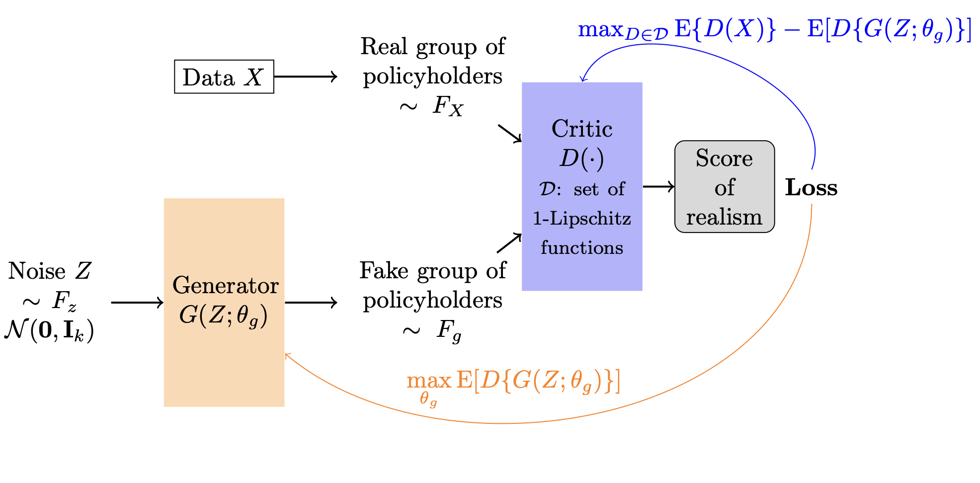
where \(\mathcal{D}\) is the set of 1-Lipschitz functions. This change in the objective function leads to the Wasserstein GAN, or WGAN. The discriminator in a WGAN is called the critic, as it outputs a real value rather than a binary classification. The WGAN is depicted schematically in Figure 1 for policyholder claim data \(X\). The black arrows represent the forward flow of information in the network, while the colored arrows represent the flow of the training process for the generator (orange) and critic (blue).

Figure 1.WGAN schema. The arrows represent the flow of the training process.

Some tactics are needed to enforce the Lipschitz constraints on \(D\). In this regard, the gradient penalty (GP) developed by Gulrajani et al. (2017) greatly improves the WGAN training. In their WGAN-GP model, the authors take advantage of the fact that a differentiable Lipschitz function has gradients with norm at most 1 everywhere. A tuning parameter \(\lambda>0\) is introduced, and the objective of the WGAN-GP is

\[\begin{align} &\min_{\theta_g}\max_{\theta_d} \mbox{E}_X\{D(X;\theta_d)\} \\&\quad- \mbox{E}_Z[D\{G(Z;\theta_g);\theta_d\}] \\&\quad+\lambda \mbox{E}_{\hat{X}}[\{||\nabla_{\hat{x}}D(\hat{X};\theta_d)||_2-1\}^2], \end{align} \]

where \(\hat{X} \stackrel{d}{=} U X+(1-U)G(Z;\theta_g)\), and \(U\) is uniformly distributed on the interval \((0,1)\), so that the distribution \(F_{\hat{x}}\) of \(\hat{X}\) is obtained by sampling uniformly along lines between pairs of points sampled from \(F_x\) and \(F_g\). For details on the motivation, the reader is referred to Gulrajani et al. (2017).

In practice, if \(m\in \mathbb{N}\) is the size of the minibatch with observations \(x_1,\ldots,x_m\), random noise vectors \(z_1,\ldots,z_m\), and independent uniform samples \(u_1,\ldots,u_m\), then we let \(\hat{x}_i=u_ix_i+(1-u_i)G(z_i;\theta_g)\) and the discriminator loss is approximated by

\[ \begin{align} \mathcal{L}_d &= \frac{1}{m}\sum_{i=1}^m -D(x_i,\theta_d)+D\{G(z_i;\theta_g);\theta_d\} \\&\quad+\lambda\{||\nabla_{\hat{x}_i}D(\hat{x}_i;\theta_d)||_2-1\}^2, \end{align} \]

while the generator loss is simply

\[\mathcal{L}_{g} = \frac{1}{m}\sum_{i=1}^m -D\{G(z_i;\theta_g);\theta_d\}.\]

Note that higher values of the critic \(D\) indicate fake samples.

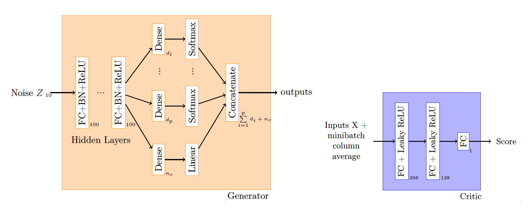
The WGAN and WGAN-GP were developed in the context of image generation tasks. However, in the current application we wish to synthesize tabular insurance data, in which some variables are categorical with multiple levels. Camino, Hammerschmidt, and State (2018) considered an application close to ours where the target data contain many multicategorical variables. They modified the WGAN-GP generator so that, after the model output, there is a dense layer in parallel for each categorical variable followed by a softmax activation function. Then, the results are concatenated to yield the final generator output.

As in Camino, Hammerschmidt, and State (2018), our generator’s architecture has one dense layer with dimension matching the number of levels for each multicategorical variable. We also add one dense layer with linear activation and dimension \(n_c\), which is equal to the number of continuous variables. The architecture of the generator and critic in our multicategorical and continuous WGAN-GP, or MC-WGAN-GP, is depicted in Figure 2. Further details about hyperparameter optimization are available in Appendix A.

Figure 2.Architecture inside the generator (orange) and the critic (blue) for our multicategorical and continuous WGAN. The dimensions \(d_1, \ldots, d_p\) represent the number of levels in categorical variables \(1, \ldots, p\). FC stands for fully connected and BN stands for batch normalization.

3. CTGAN

Another possible path to simulating insurance claim data is through a conditional tabular GAN or CTGAN (L. Xu et al. 2019). This method was applied to ratemaking data in Kuo (2019). Additionally, Kuo developed an R wrapper for this software to make it easily accessible to insurance practitioners more familiar with R than Python. Starting from his code, we slightly adjusted the preamble to improve the application consistency on our machines and slightly adjusted the preprocessing, but other than that the overall code remained the same. Our version of the code is available in the GitHub repository for this paper.

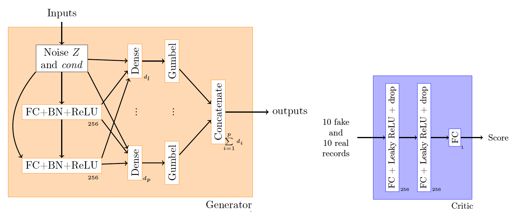
The CTGAN simulates records one by one. It first randomly selects one of the variables (say fuel type: diesel or gasoline). Then, it randomly selects a value for that variable (say diesel). Following Kuo (2019), we use the true data frequency to sample the value rather than the log-frequency, as suggested in L. Xu et al. (2019). Given that value for that variable, the algorithm finds a matching row from the training data (in this example, it randomly selects a true observation with a diesel-powered car). It also generates the rest of the variables conditioning on it being diesel-powered. The generated and true rows are sent to the critic, which gives a score. Figure 3 summarizes the CTGAN procedure.

Figure 3.CTGAN schema. The model flow is illustrated for the case when the selected column is Fuel Type and the selected value for that column is Diesel.

Figure 4 zooms inside the architecture of the generator and critic. Both the critic (blue) and generator (orange) use two fully connected layers to attempt to capture all relationships between the columns. An additional sophistication of the CTGAN is the use of the PacGAN framework (Lin et al. 2018) in the discriminator, where 10 samples are provided in each pac to prevent the mode collapse issue. As in D. Xu et al. (2018), the model is trained using the WGAN-GP loss.

Figure 4.Architecture inside the CTGAN generator (orange) and critic (blue). The dimensions \(d_1, \ldots, d_p\) represent the number of levels in categorical variables \(1, \ldots, p\). The input of the generator is Gaussian random noise and the condition cond of the feature value that was randomly selected (see Figure 3). FC stands for fully connected, BN for batch normalization, Gumbel for the Gumbel softmax activation, and drop for dropout.

Like the previously discussed MC-WGAN-GP, the CTGAN does not incorporate privacy protections, though that could possibly be developed, as hinted in Kuo (2019).

4. MNCDP-GAN

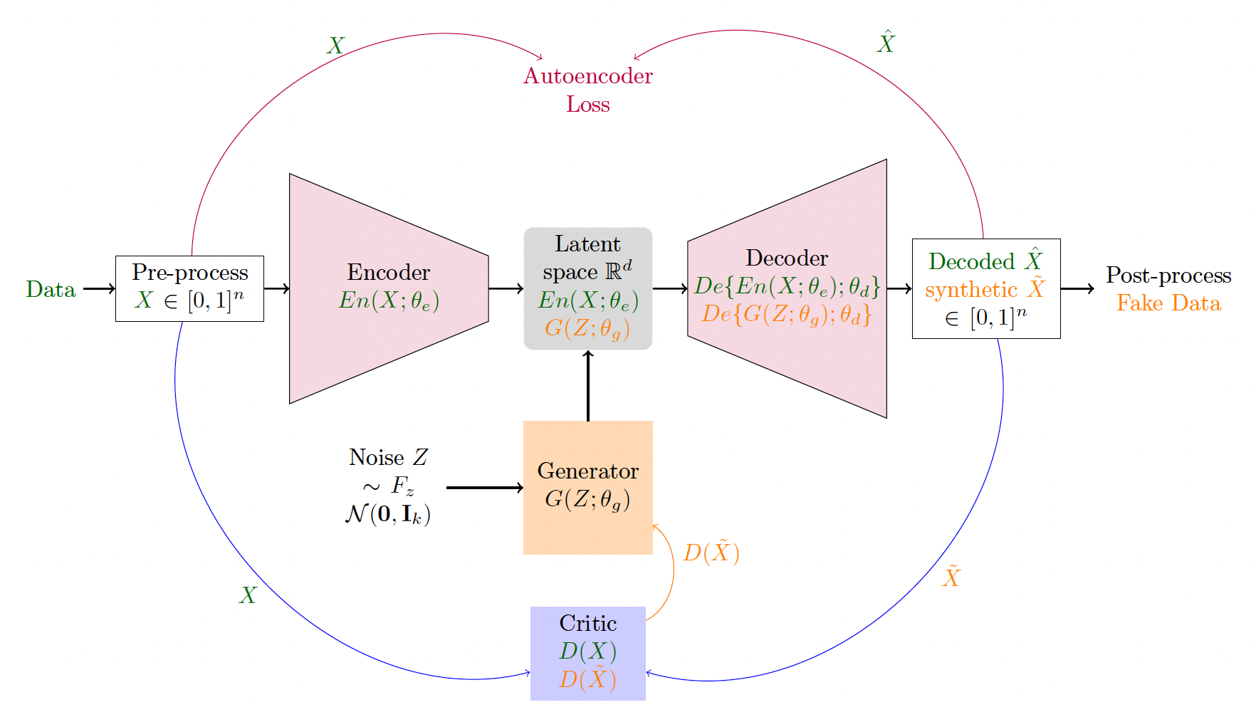
The mixed numerical and categorical differentially private GAN (MNCDP-GAN) tries to solve the drawbacks of the other two GANs. The MNCDP-GAN includes an autoencoder and a WGAN. The main advantage of this architecture, introduced in Tantipongpipat et al. (2019), is that the generator works in a latent space of encoded variables, which can be easier to model adequately than the original structured data. Training can be done in a differentially private (DP) manner, allowing a DP guarantee on the generated dataset.

As depicted in Figure 5, the original data are first preprocessed (one-hot encodings for categorical variables and either binning or min-max standardization for continuous variables), resulting in vectors defined in \([0,1]^n\) that are fed into an encoder, shrinking the dimension to \(d<n\), a hyperparameter. Then, a decoder enters the encoded variable in the latent space \(\mathbb{R}^d\) and outputs data in the format \([0,1]^n\), which is subsequently postprocessed to deliver data in the original format. This architecture is called an autoencoder and is used in many neural network applications. In our context, the autoencoder creates the latent space in dimension \(d\), which is easier for the generator to learn because it has less structure than the original data space. The generator takes in random noise and outputs a vector in the latent space, which can then be decoded by the decoder to produce a synthesized record. The critic is trained with the Wasserstein loss and compares the generated data before postprocessing with the preprocessed original data.

Figure 5.MNCDP-GAN schema. The orange relates to the generated data, and the green relates to the original data. The colored arrows represent the flow into the loss for the training of each network, with autoencoder in red, generator in orange, and discriminator in blue. For DP training, noise is added in training the decoder and the critic.

In Figure 5, the autoencoder flow and training are depicted in red, the data flow in the autoencoder and critic is indicated in green, and the generated data flow through the decoder and the critic is highlighted in orange. It is reasonably assumed that the postprocessing step can be done using public knowledge and does not affect the model’s DP quality. The DP training is done by injecting noise in the decoder and critic. For more details, refer to Tantipongpipat et al. (2019).

The level of differential privacy achieved by the model (including both the autoencoder and the GAN) is quantified by the value \(\epsilon>0\). This value relates to how different an analysis may be if one data point is added or removed. If the dataset \(X'\) is identical to \(X\) except for one added data point, then an \((\epsilon,\delta)\) differentially private analysis \(\mathcal{M}\) satisfies

\[\Pr\{\mathcal{M}(X)\in S\} \leq e^{\epsilon}\Pr\{\mathcal{M}(X')\in S\}+\delta,\]

for \(\delta>0\), any such \(X,X'\) and \(S\subseteq Range(\mathcal{M})\), as seen, for example, in Dwork and Roth (2014). A smaller \(\epsilon\) represents stronger privacy guarantees, but comes with decreased performance for synthesizing realistic data because more noise is added to the training. The values of \(\epsilon\) and \(\delta\) for our procedure are obtained through a privacy accountant as explained in Tantipongpipat et al. (2019). Further details on our implementation are available in Appendix B.

5. Case study

To show the value of the three approaches in a reproducible manner and compare their effectiveness in producing synthetic data, we use a well-known publicly available dataset for the case study. The dataset contains a set of 412,748 French motor third-party liability policies observed in a single year (Dutang and Charpentier 2019). The data contain the number of claims (ClaimNb), along with eight explanatory variables:

• Exposure: the number of car-years on the policy, bounded between 0 and 1 (we removed the few records with Exposure greater than 1)

• Power: an ordered categorical variable that describes the power of the vehicle

• CarAge: the vehicle age in years

• DriverAge: the age of the primary driver, in years

• Brand: the vehicle brand divided into the following groups: A— Renault, Nissan, and Citroen; B— Volkswagen, Audi, Skoda, and Seat; C— Opel, General Motors, and Ford; D— Fiat, E— Mercedes, Chrysler, and BMW; F— Japanese (except Nissan) and Korean; G— other

• Gas: diesel or regular

• Region: the policy region in France

• Density: number of inhabitants per km\({\mathstrut}^2\) in the home city of the driver

Brand, Gas, Power, and Region are all categorical variables and the other four are numeric (continuous or discrete). For the MNCDP models we show four DP levels:

• \(\epsilon = \infty\) is labeled on the plots as “MNCDPInfty”: no differential privacy

• \(\epsilon = 100,000\) labeled as “MNCDP100k”

• \(\epsilon = 10,000\) labeled as “MNCDP10k”

• \(\epsilon = 5\) is labeled as “MNCDP5”: strong differential privacy

We simulate a dataset of the same size as the original dataset using each of the GANs and compare the univariate distributions in the generated samples with the univariate distributions in the real data. If the methods faithfully reproduce the original data, we expect the distributions to be similar.

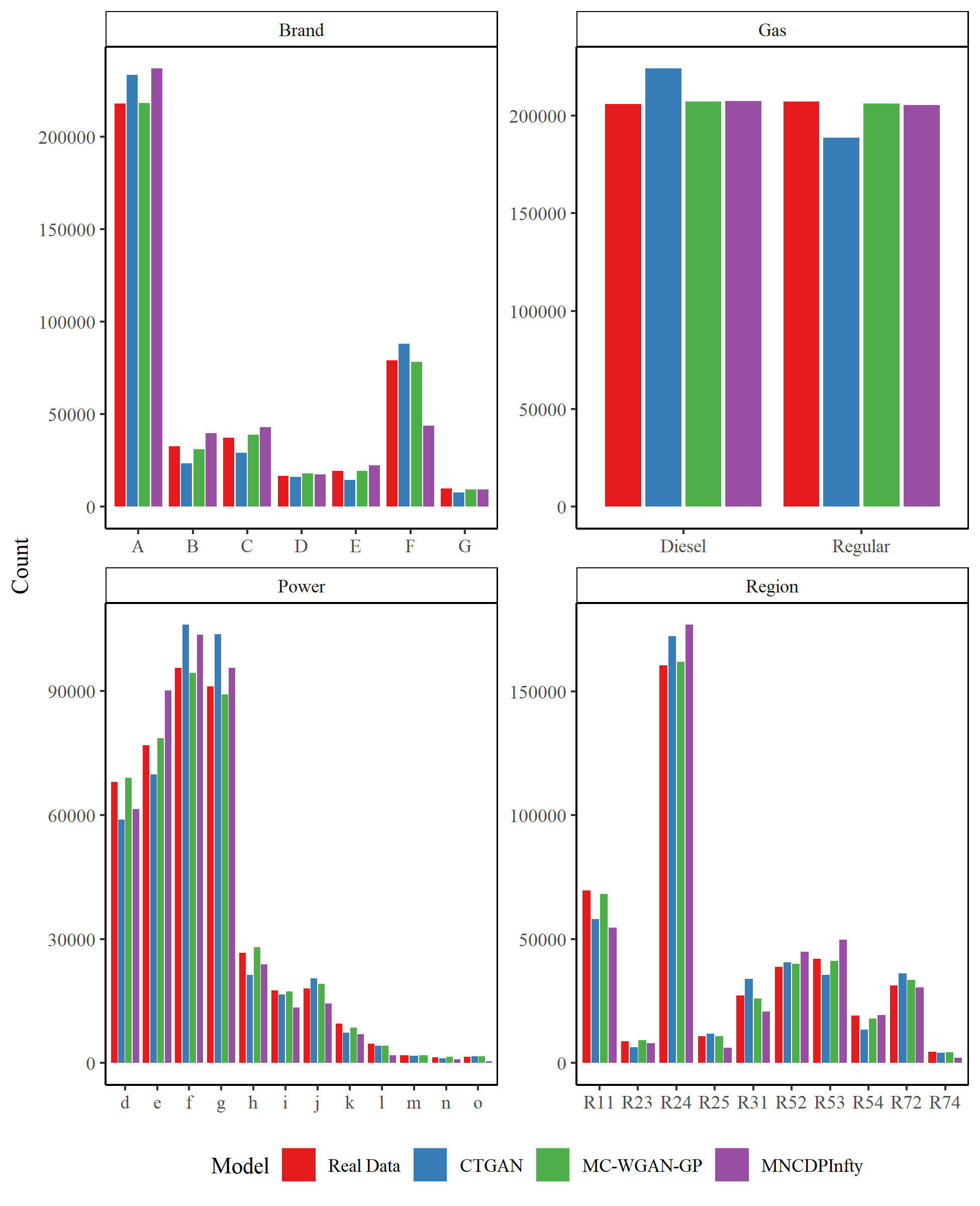
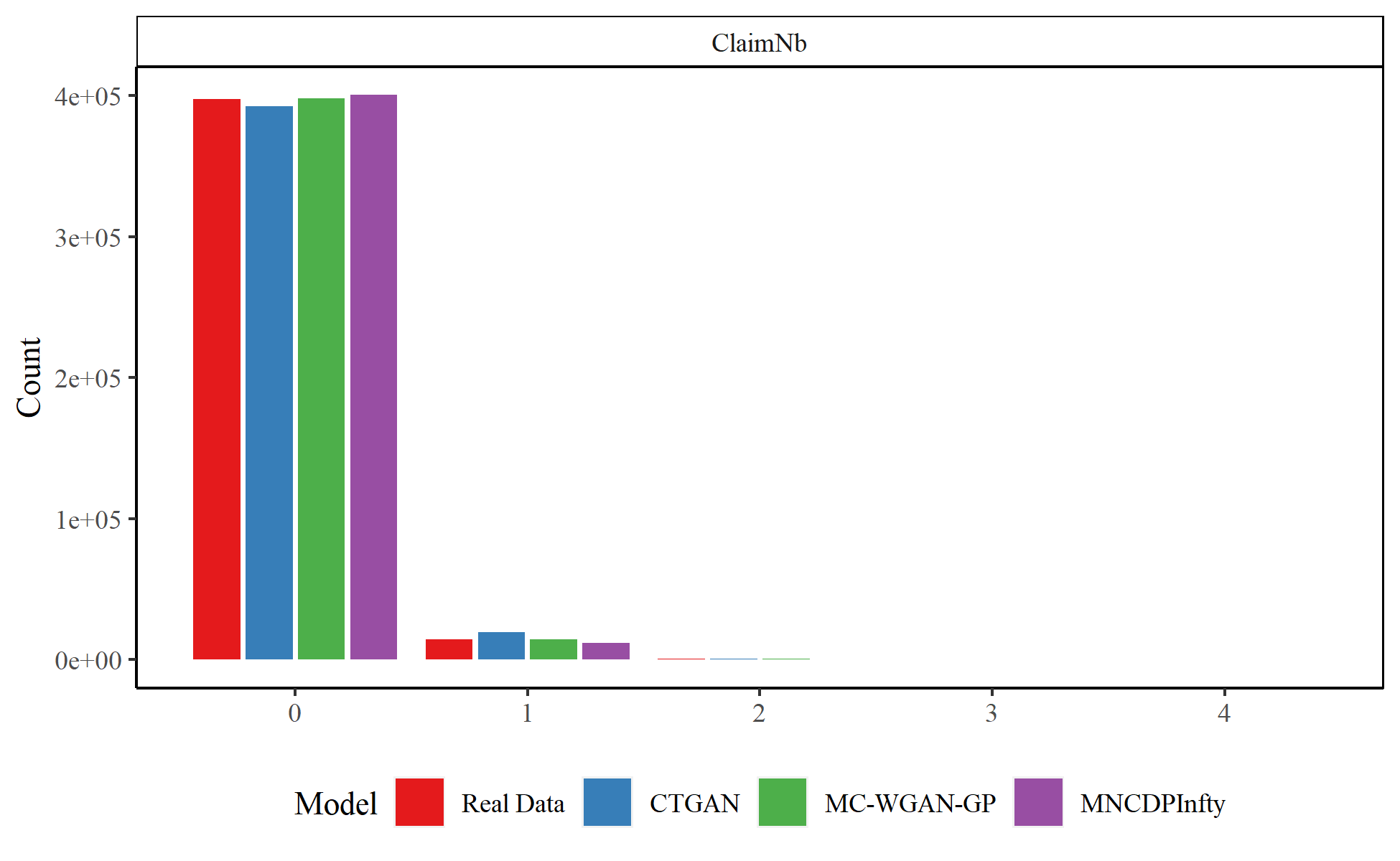
We first compare the results for the categorical variables. Figure 6 shows the observations in each category in the real and generated datasets for Brand, Gas, Power, and Region for the real data, the MC-WGAN-GP, the CTGAN, and the MNCDP-GAN without DP. Figure 7 provides the same information on the number of claims. From the univariate perspective, the three models all replicate the real data reasonably well. In particular, the MC-WGAN-GP (green) closely reproduces the univariate distributions in the real data (red) for these four categorical variables and the response variable.

Figure 6.Comparison of univariate categorical variable distributions.

Figure 7.Comparison of response variable distributions.

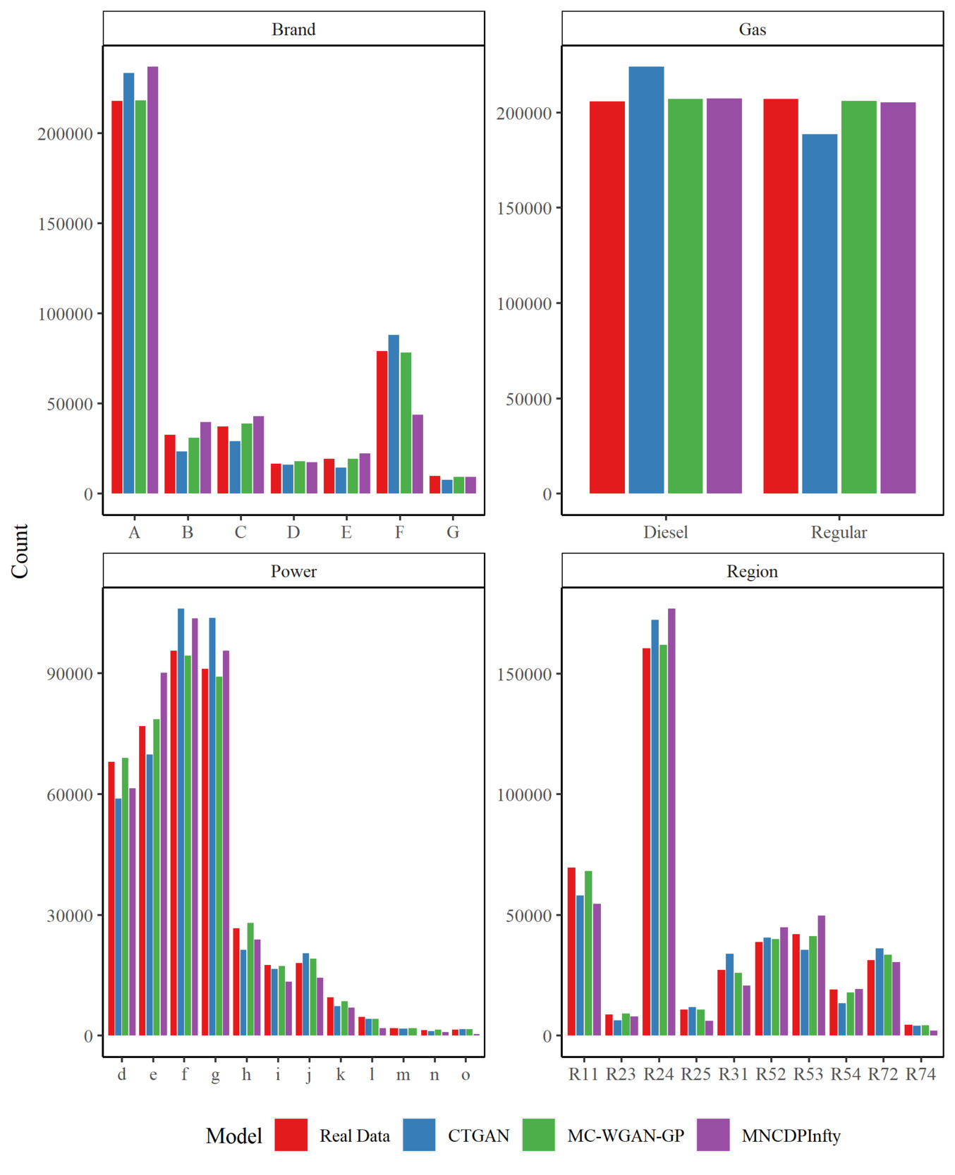
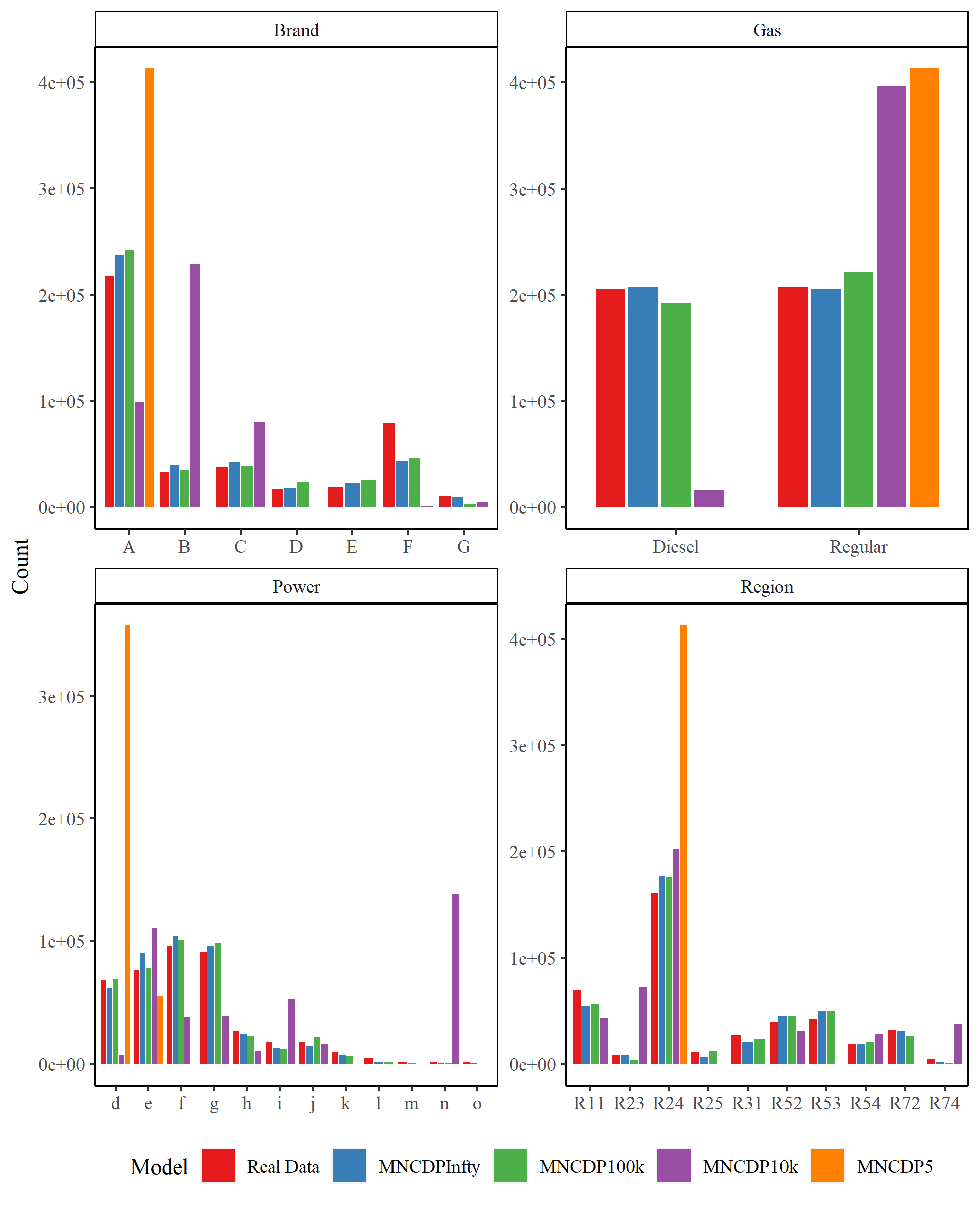
Figure 8 shows the same information as Figure 6, but for the MNCDP model with varying levels of differential privacy. It is readily apparent that the quality of synthesized data declines markedly as the level of differential privacy increases. Again, the model with \(\epsilon = \infty\) (MNCDPInfty), no differential privacy, follows the data rather well. As \(\epsilon\) decreases to 100,000 (MNCDP100k), the model still approximates the real data relatively well. But the synthetic data when \(\epsilon=10,000\) (MNCDP10k) and, especially, \(\epsilon = 5\) (MNCDP5) are not close to the real data. The noise added to the process in both cases completely obscures the original signal. This is a consistent result throughout our case study.

Figure 8.Comparison of univariate categorical variable distributions for MNCDP-GAN models with \(\epsilon \in\{5,10000,100000, \infty\}\).

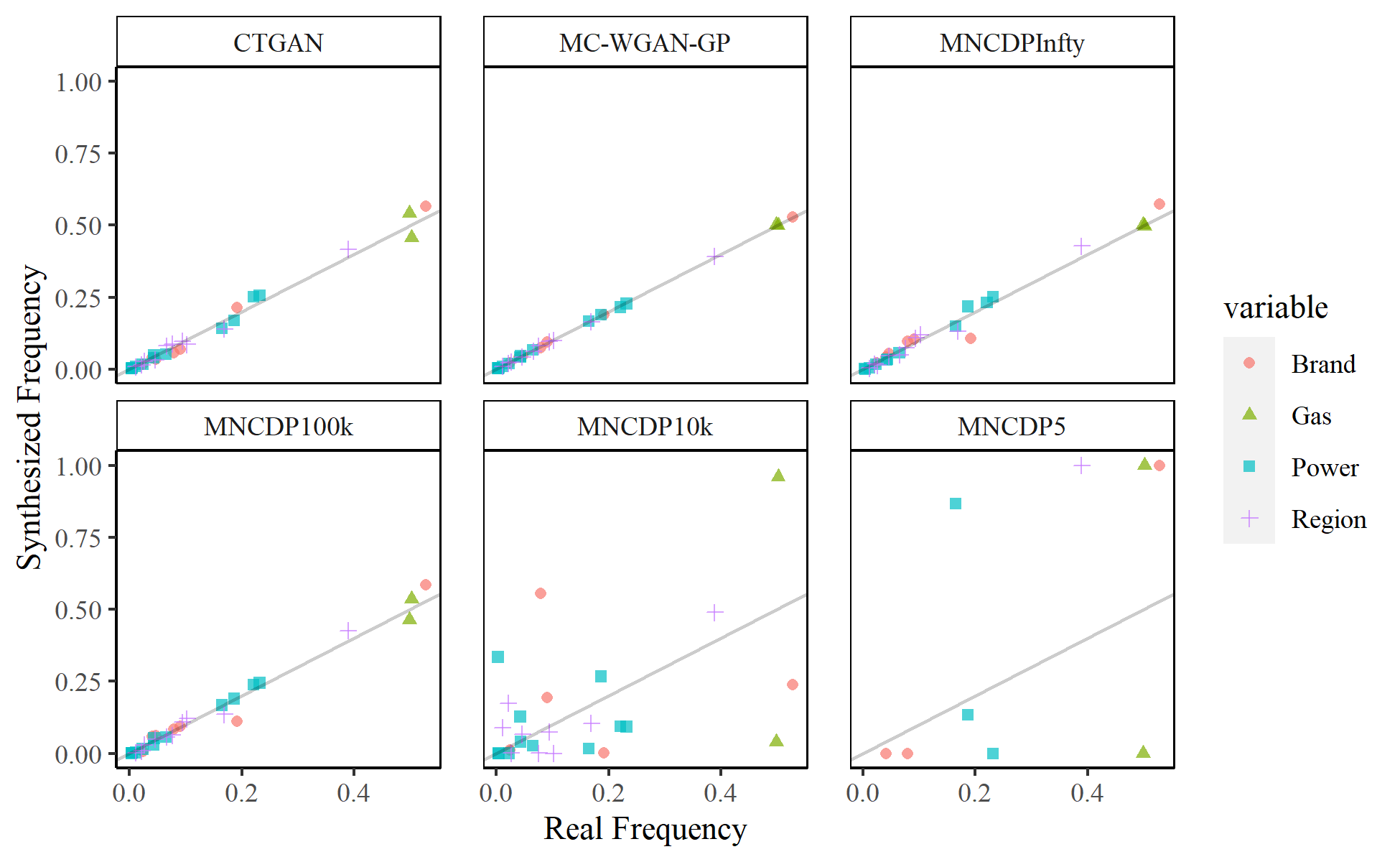
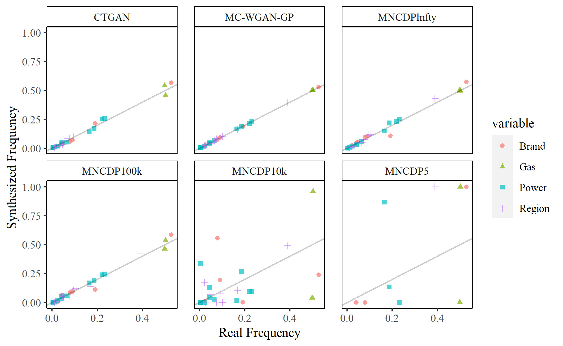
Shown another way, Figure 9 plots the frequency for each category in the real data on the \(x\)-axis against the frequency in the synthesized data on the \(y\)-axis for each of the GANs we considered, color-coded by feature. The line \(y=x\) is also plotted. The MC-WGAN-GP dataset seems to match the real frequencies best, followed by the CTGAN, MNCDPInfty, and MNCDP100k models (which are relatively similar). As noted above, the MNCDP10k and MNCDP5 models drastically differ from the original data.

Figure 9.Comparison of the synthesized and real group frequencies for each class of the four categorical variables.

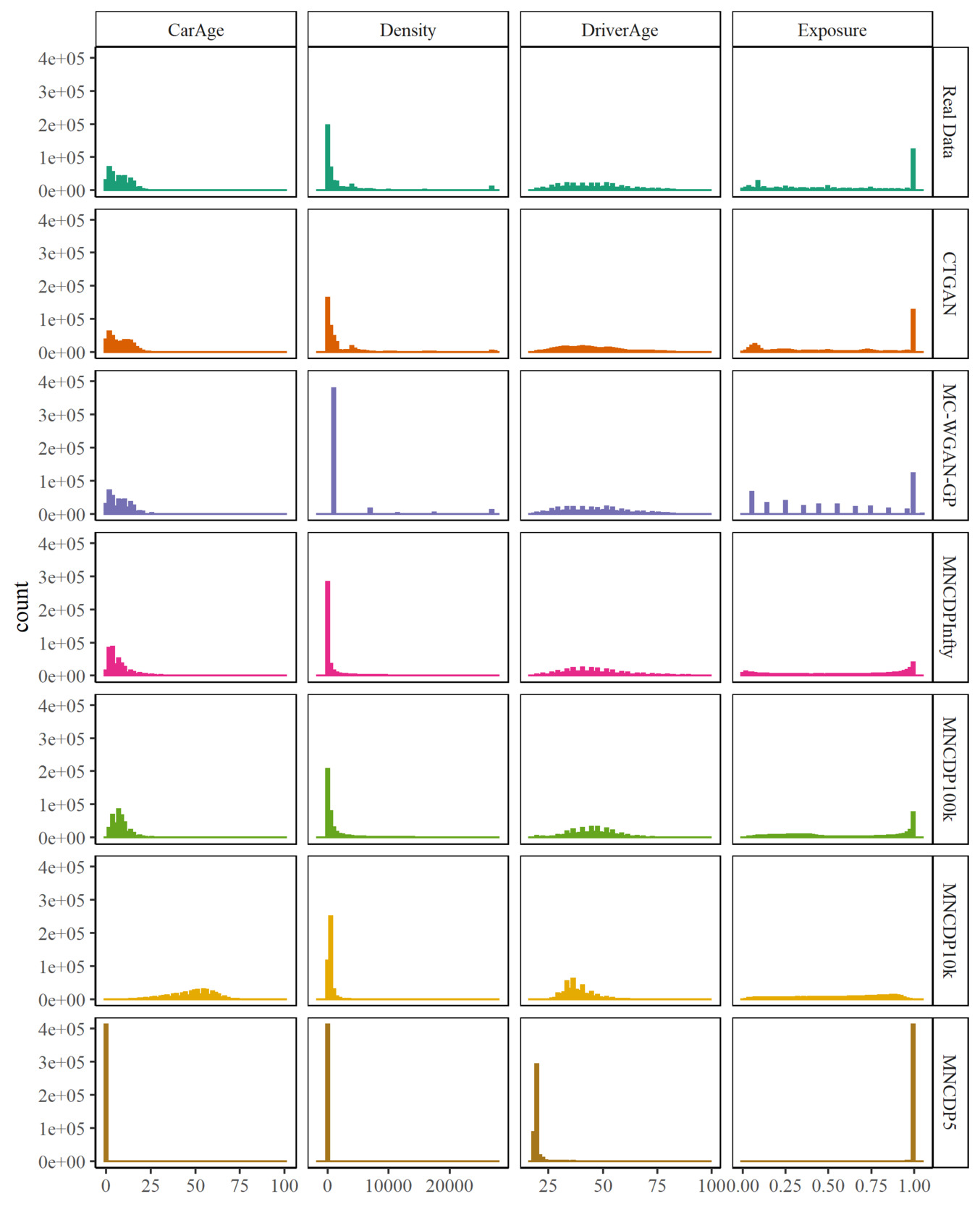
For the numeric variables CarAge, Density, DriverAge, and Exposure, Figure 10 shows the distributions of the real data in the top row and compares them with the distributions of data generated by the models. The Exposure variable is one of the most difficult aspects of insurance data because a large proportion of Exposure values are exactly one. After accounting for those, the remaining Exposure values tend to be either close to zero or close to monthly intervals (1/12, 2/12, 3/12, etc.). Both the CTGAN and MC-WGAN-GP do well with synthesizing the correct number of 1 values, but in the rest of the distribution, the MC-WGAN-GP is too bumpy and the CTGAN might be too smooth. CTGAN is the best model for the Density variable. Both DriverAge and CarAge are matched well by all three methods.

Figure 10.Comparison of univariate numerical variable distributions.

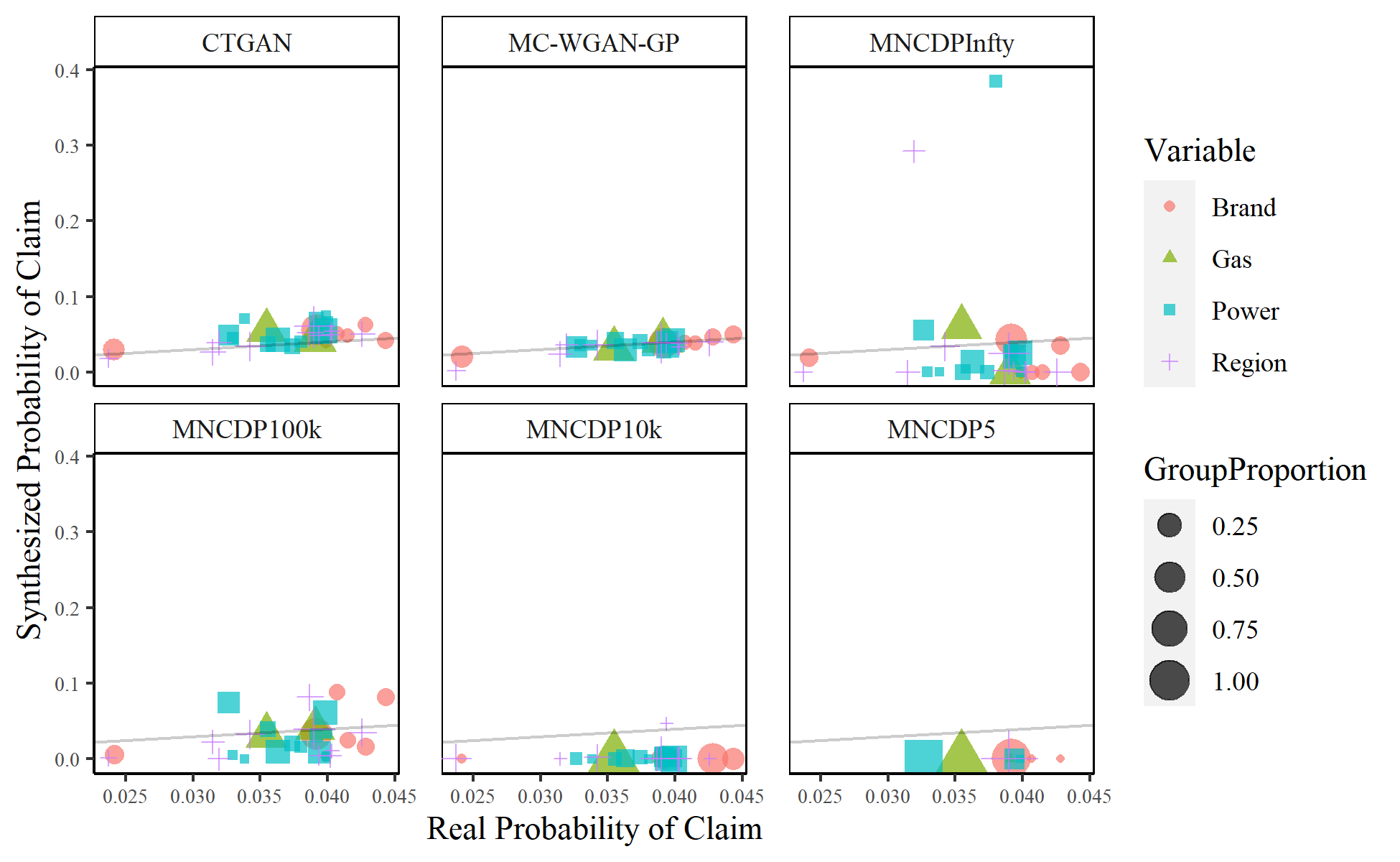
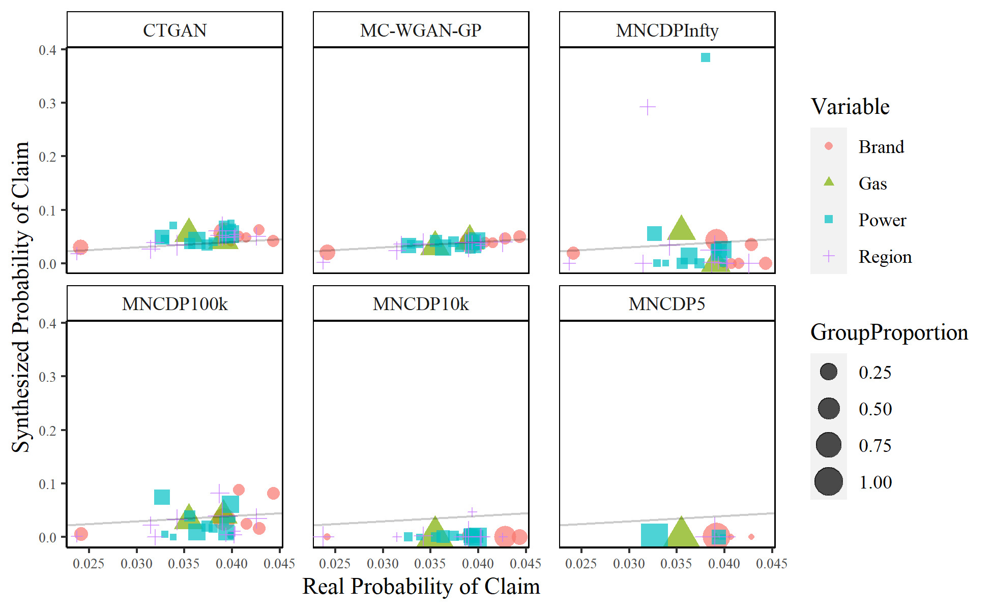
It is important to correctly model the univariate characteristics, but it is even more important to correctly model the multivariate relationships. This is especially true with the relationship between claim counts and the various explanatory variables. Figure 11 compares the probability of a claim in each categorical group. The real probability of a claim is on the \(x\)-axis, with the synthesized probability on the \(y\)-axis. The line \(y=x\) is also plotted to show the ideal goal. The size of the marks shows the proportion of synthesized data in each group. By this metric, the MC-WGAN-GP performs the best, followed closely by the CTGAN. The MNCDP-GAN does not perform well, even without differential privacy.

Figure 11.Comparison of the synthesized and real empirical probability of a claim for each group.

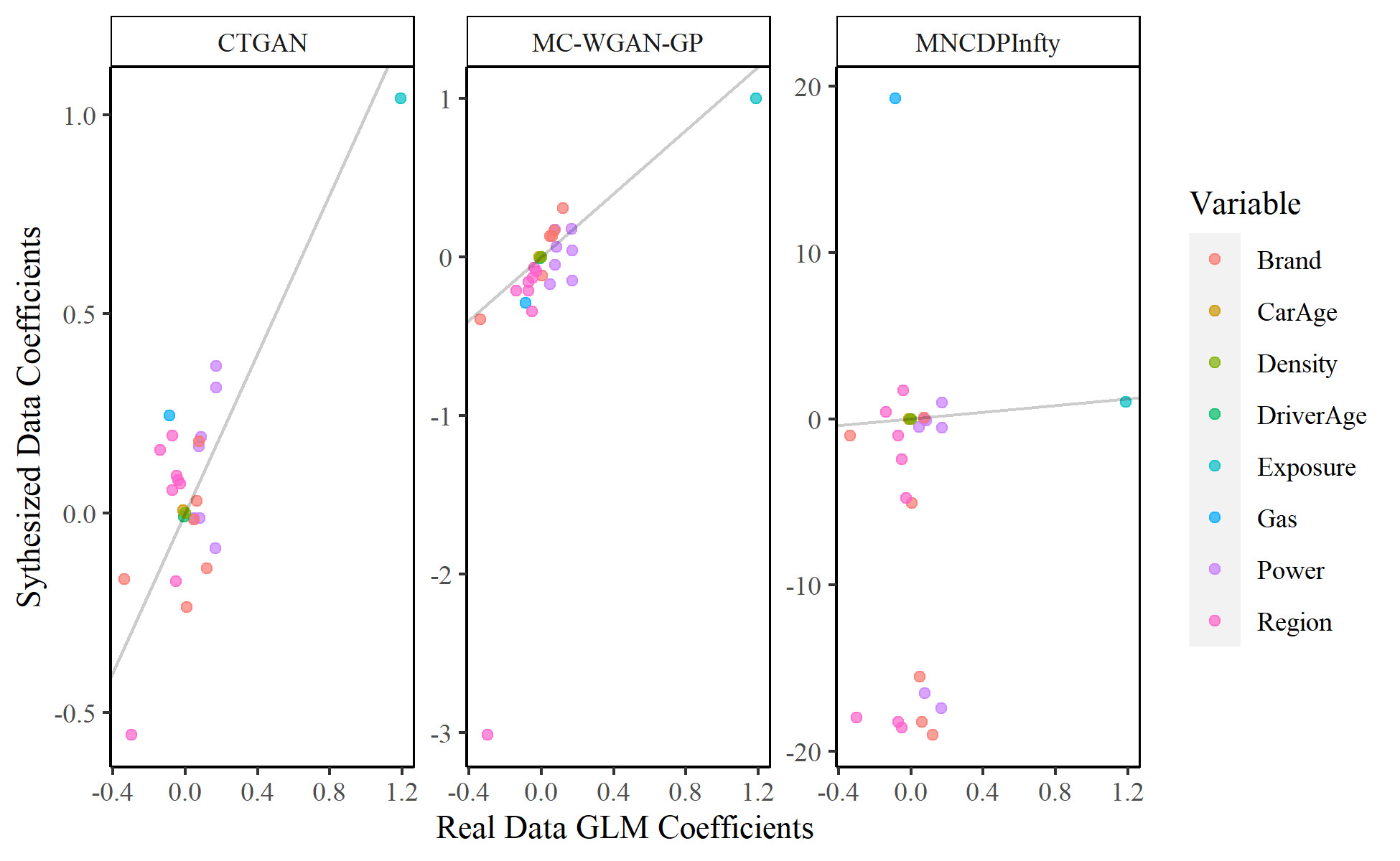
Our last test examines the consistency of models fitted on the original and synthesized data. We split the real data into two parts, a 70% training set and a 30% test set. We fit a Poisson generalized linear model on the training set, predicting the number of claims using all eight explanatory variables. We then fit the same model on a 70% sample from each of the synthesized datasets. The sampling and model fitting are performed 5,000 times to examine the sampling variability and to obtain more consistent estimates. Figure 12 compares the average estimated regression coefficients for each of the three models. We find that the CTGAN coefficients are all close to the real coefficients. The coefficients estimated with the MC-WGAN-GP data are similarly close, except for a single region coefficient. The results achieved using the MNCDP synthesized data are again the worst.

Figure 12.Comparison of the Poisson regression coefficients for the synthesized and real data.

With each fitted model, we then predict the claim counts for the 30% real test data and compare the predictions from the models fit on the synthesized data to the predictions from the models fit on the real data. Table 1 shows the median absolute error (MAE) and mean squared error (MSE) between the predictions, with 95% bootstrapped confidence intervals. The MC-WGAN-GP significantly outperforms the other two models on both metrics. The CTGAN performs next best, and the MNCDP-GAN again shows the worst performance.

6. Conclusion

In this paper, we presented, implemented, and compared three methods to synthesize insurance data. All three methods were based on GANs, and each method had advantages and disadvantages. The MC-WGAN-GP method synthesized the most realistic data, generating data that were very similar (accounting for both univariate and multivariate relationships) to the real data. The CTGAN method was the easiest to use, especially for individuals more familiar with R than Python. The data synthesized by CTGAN were almost as good as the MC-WGAN-GP data. The main drawbacks of MC-WGAN-GP and CTGAN were that they provided no privacy guarantees; some records in the generated data could still contain confidential information. The MNCDP-GAN incorporated differential privacy, but its synthesized data (even without differential privacy) were not as good as those produced by the other two methods.

Future work can start from any of the three models and attempt to add the advantages of the other two—that is, either add differential privacy and ease of use to the MC-WGAN-GP, add improved synthesis and differential privacy to the CTGAN, or add improved synthesis and ease of use to the MNCDP-GAN. In any case, GANs are a promising tool for synthesizing and protecting private data that are important to actuarial science and other fields.

Acknowledgments

This work was supported by a Casualty Actuarial Society (CAS) Individual Grant and by M.-P. Côté’s Chair in Educational Leadership in Big Data Analytics for Actuarial Sciences — Intact. The authors thank the members of the CAS project oversight committee, Syed Danish Ali, Morgan Bugbee, Marco De Virgilis, and Greg Frankowiak, for useful feedback throughout the project. The project would not have been possible without the computing resources provided by the Digital Research Alliance of Canada, and the statistics department computing cluster at Brigham Young University.