Development of Telematics Safety Scores in Accordance with Regulatory Compliance

1. Introduction

Telematics automobile insurance, also known as usage-based insurance, leverages technology to monitor driving behavior and adjust policy premiums accordingly. Such coverage involves the use of telematics devices to collect real-time driving data, which distinguishes it from traditional auto insurance, which relies only on demographic features and historical claims data. The detailed information on driving behavior allows insurers to assess risk more accurately and incentivizes safe driving by offering discounts to policyholders showing low-risk driving behavior. Telematics insurance’s appeal is echoed by its significant growth in North America, Europe, and other regions. According to Research and Markets, the market size of telematics insurance was USD 4.77 billion in 2024 and will grow at an annual rate of 18.92%, reaching USD 13.77 billion by 2030. However, integrating telematics information into insurance pricing introduces new challenges in privacy, data usage policies, fairness and discrimination issues, and ethical concerns (Handel et al. 2014). These challenges, in turn, compel regulators to establish new requirements on the collection and use of telematics data by insurers.

Telematics data encompasses a wide range of driving behaviors, such as speed, acceleration and breaking patterns, turning radius, and operating hours, among other factors. Recent studies have demonstrated the usefulness of telematics data in risk assessment and ratemaking—see, for instance, Verbelen, Antonio, and Claeskens (2018), Ayuso, Guillen, and Nielsen (2019), Arumugam and Bhargavi (2019), Denuit, Guillen, and Trufin (2019), Guillen et al. (2019), Huang and Meng (2019), Pesantez-Narvaez, Guillen, and Alcañiz (2019), So, Boucher, and Valdez (2021a), Che, Liebenberg, and Xu (2022), and Henckaerts and Antonio (2022). Specifically, G. Gao, Meng, and Wüthrich (2022) and Y. Gao, Huang, and Meng (2023) show that using telematics data leads to a more precise prediction of the key features that are crucial for identifying high-risk drivers. Given such dominant evidence supporting the use of telematics data, we will utilize telematics features, along with traditional features, to adjust premiums in the proposed framework. However, we face two immediate questions in this endeavor:

1. How do we build a ratemaking model that uses telematics features?

2. How can we ensure the compliance of the model with telematics regulations?

The current literature on telematics insurance mostly focuses on addressing the first question (Q1) but, to the best of our knowledge, completely ignores question two (Q2). This motivates us to propose an insurance ratemaking framework that makes use of new telematics features and, at the same time, complies with the related regulatory requirements. As it turns out, the compliance requirement has a direct impact on how our proposed framework uses telematics information.

Before we introduce our framework, we briefly review several mainstream approaches (that is, answers to Q1) that process telematics data in insurance. One straightforward, perhaps less sophisticated, approach is to integrate telematics features directly with traditional features and use them together in a standard model—in that respect, see Ayuso, Guillen, and Nielsen (2019) and Peiris et al. (2024). Because of the often high-dimensional nature of telematics datasets, applying dimension-reduction techniques when processing the data can be beneficial. Indeed, Jeong (2022) and Chan et al. (2024) show that doing so improves model performance and interpretability. Given the complexity of telematics data, it is not surprising that various machine learning methods, such as neural networks, find great application in telematics insurance (G. Gao, Wang, and Wüthrich 2022; Dong and Quan 2025). In our proposed framework, we use a feedforward neural network (FNN), a special type of neural network, to help process telematics information.

Given the general nature of Q2, a universal answer is unlikely, and a case-by-case approach is more suitable to address that question. As such, we take as our motivation a bill addressing telematics automobile insurance introduced in the 2023–2024 session of the New York State legislature, Assembly Bill 2023-A7614. Clause (D) of that bill prohibits “a premium increase for a driver or vehicle due to a telematics program that measures driving behavior during the current policy period.” This particular provision motivates us to impose a discount-only constraint on telematics policies.^[1] As hinted earlier, such a constraint leads to two significant challenges or consequences. First, because of the complexity and high dimensionality of telematics data, it is nontrivial to propose a model that satisfies the discount-only constraint. Second, the constraint would likely prompt insurers to increase the base premium and would lead to favorable selection bias—that is, drivers with low-risk driving behavior would be more likely to enroll in a telematics policy (Cather 2020).

Having discussed the background and motivation, we now introduce our ratemaking framework for claim frequency. To utilize both traditional and telematics features, we turn to a standard (Poisson) generalized linear model (GLM) with risk embedding via an FNN. To be precise, we use an FNN to build a map from the available telematics features \(y\) to a safety score \(R\), that is, \(R = f(y)\), in which \(f\), referred to as the risk-embedding function, is learned by the FNN. Next, we propose a modified GLM that takes the safety score \(R\), along with the recorded traditional features \(x\), as input, which reads as \(\log \mu = \alpha + \beta R + \gamma x\), with \(\mu = \mathbb{E}[N]\) denoting the expected claim frequency. With the dimension reduction (\(y\) is a high-dimensional vector, but \(R = f(y)\) is a one-dimensional scalar) and the above GLM, the discount-only constraint is satisfied if we impose \(f(\cdot) \ge 0\) and \(\beta < 0\) (which together generate a nonpositive component \(\beta R\) in the GLM). As is obvious, the choice of a risk-embedding function \(f\) plays a key role in our framework, and we propose two methods, both based on an FNN, to compute the safety score \(R = R^{(i)}\), \(i = 1, 2\) (see equations (6) and (7) in Section 2 for details). Note that the modified GLM with each \(R^{(i)}\) yields a model under the proposed framework, and we consider two such models in this paper.

To test the performance of the two proposed models, we compare them with two benchmark models: Model 1 is a Poisson GLM that uses only the traditional features (\(\log \mu = \alpha + \gamma x\)); Model 2 is a Poisson GLM that uses both the traditional and telematics features in a parallel manner (\(\log \mu = \alpha + \gamma x + \eta y\)). We show that the proposed models, with a suitable safety score \(R\), outperform the benchmark models in both in-sample goodness of fit and out-of-sample prediction. We also find that the discount-only constraint on telematics insurance could lead to a potential increase of the base premium for certain groups (high-risk drivers). In addition, when there is a relatively high degree of favorable selection (that is, good drivers are more likely than bad drivers to choose telematics insurance), the discount-only requirement works as desired by rewarding low-risk drivers, but not at the cost of raising premiums for high-risk drivers.

The paper contributes to a growing body of literature on telematics insurance from a unique perspective—regulatory compliance. To the best of our knowledge, it is the first paper to take into account proposed regulatory requirements on insurers’ use of telematics data. Motivated by the discount-only constraint drawn from the introduced New York Assembly Bill A7614, we propose a general ratemaking framework that incorporates the predictive advantage of telematics information and complies with the discount-only regulatory provision. We remark that the proposed framework can be easily modified to accommodate a quantitative, not just a directional (no increase), requirement on the premium of telematics policies. Indeed, we can scale the safety score \(R\) to a closed interval (say \([0,1]\)) and impose a threshold on \(\beta\) to limit the impact of the telematics data to achieve any desired bound set by regulators.

The remainder of the article is organized as follows. We introduce our ratemaking framework in Section 2 and test the performance, both in sample and out of sample, of two specific models under the proposed framework in Section 3. We dedicate Section 4 to the study of selection biases on the implied relativities for the telematics policies. We conclude in Section 5.

2. Framework

This section introduces a ratemaking framework for claim frequency that utilizes telematics features in the dataset and complies with a discount-only regulatory requirement—such as was proposed in New York Assembly Bill 2023-A7614—that prohibits premium surcharges in the current policy period based on telematics data.

We consider an automobile insurance portfolio with traditional features (such as gender, age, vehicle information, etc.) and telematics features (such as sudden acceleration and braking, turning speed, time and day of driving, etc.); there are \(I \in \mathbb{N}\) policyholders in the insurance portfolio. For every policyholder \(i\), \(i=1, \dots, I\), denote their data entry in the portfolio by \((x_i, y_i; N_i)\), where \(x_i \in \mathbb{R}^m\) and \(y_i \in \mathbb{R}^n\) record their traditional and telematics features, respectively, and \(N_i\) is the claim frequency. We often suppress the subscript \(i\) when we consider a generic policyholder. Since the collection of telematics data is often optional and requires the policyholder’s consent, it is expected that telematics information is available only on a subset of the entire insurance portfolio.

We start by reviewing two existing approaches that use telematics features in ratemaking. The first, and less sophisticated, approach is to treat both traditional and telematics features in the same way and adopt the following GLM:

\[\log \mu_i = \alpha + \eta \cdot y_i + \gamma \cdot x_i, \tag{1}\]

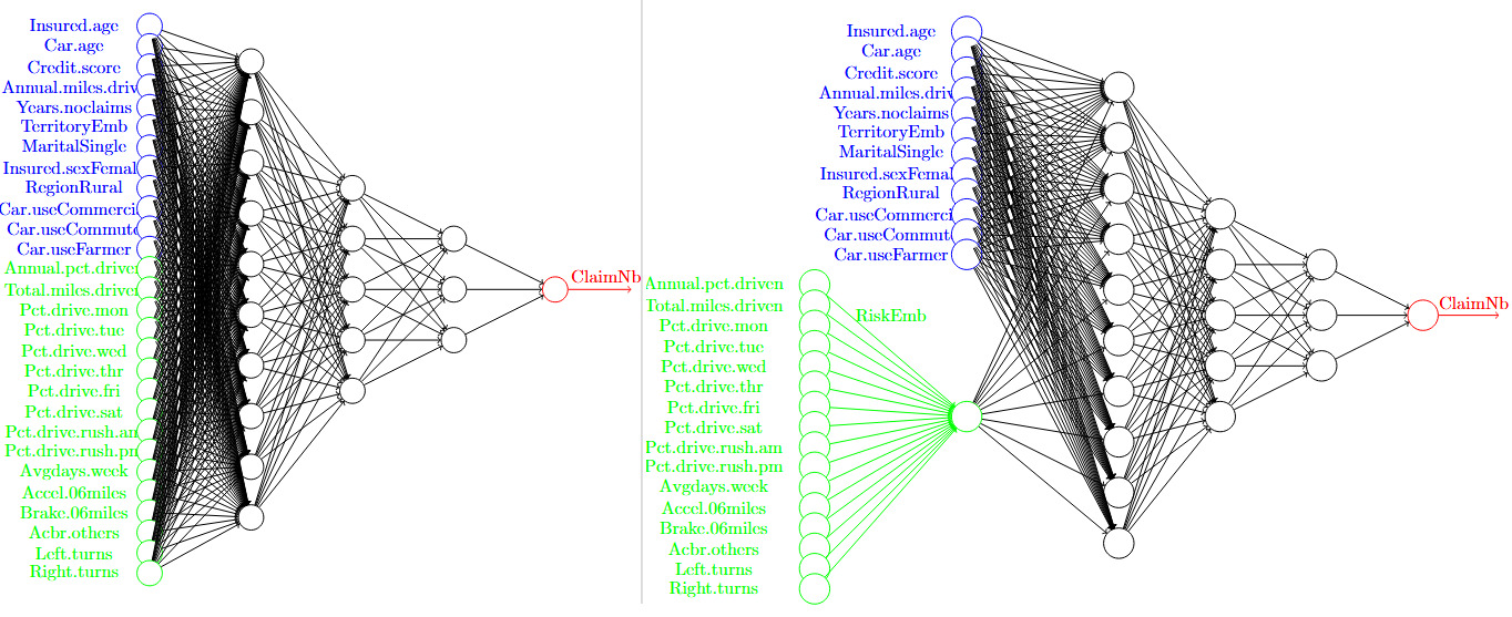
in which \(\alpha \in \mathbb{R},\, \eta \in \mathbb{R}^n, \, \gamma \in \mathbb{R}^m\) are regression parameters, and \(\mu_i = \mathbb{E}[N_i]\) denotes the expected claim frequency of policyholder \(i\) and is connected to the linear predictor \(\alpha + \eta \cdot y_i + \gamma \cdot x_i\) via the canonical link function (which is set to be the log function here). The second, and more modern, approach is to use a machine learning technique that relaxes the linear structure in the GLM (1). Along this direction, one may directly combine the traditional and telematics features to fine-tune an FNN for the ratemaking purpose. We illustrate one example of this approach in the left panel of Figure 1. However, due to the “black-box” nature of neural networks, this approach will likely fail the regulatory requirements regarding the use of telematics data in insurance ratemaking.

Figure 1.Examples of FNN architectures with both traditional and telematics features.

Note: In the left panel, the telematics features are used directly, in the same way as traditional features, to train the FNN. In the right panel, the telematics features are first transformed into a safety score via a hidden layer; next, the safety score and the traditional features are used to train the FNN.

To address the noncompliance drawback of the existing approaches reviewed above, we propose a two-step modeling approach, described as follows. The first step is to make use of the available telematics features in the dataset. To that end, we modify the standard GLM and propose the following model:

\[\log \mu_i = \alpha + \beta R_i + \gamma \cdot x_i, \quad \text{with } R_i = f(y_i),\tag{2}\]

in which \(f(\cdot) : \mathbb{R}^n \mapsto \mathbb{R}\) is a risk-embedding function. Comparing the modified GLM above in (2) with the standard GLM in (1), the essential difference is that we do not directly regress the telematics features \(y\) but instead apply a risk-embedding function \(f\) to reduce the multidimensional features \(y\) into a one-dimensional scalar \(R = f(y)\), which we call the safety score, and then use the transformed safety score \(R\), along with the traditional features \(x\), in the regression. We will discuss how we compute the safety score later.

In the second step, we “translate” the regulatory requirements into mathematical conditions and impose them on the risk-embedding function \(f\) and/or the regression parameters in (2). In this way, the modified GLM in (2), together with appropriate regulatory constraints, will fully comply with the regulations on telematics data in insurance ratemaking. In this work, we are particularly interested in the discount-only regulatory requirement on telematics policies. For that purpose, we impose the following constraints on (2):

\[\begin{aligned} f(\cdot) \ge 0 \quad \text{and} \quad \beta < 0 . \end{aligned}\tag{3}\]

We easily see that, all things being equal, the combined constraints in (3) produce a nonpositive component \(\beta R_i\) in (2), which can be seen as a “discount” in premium to telematics policies. Note that with the constraints (3) in force, the smaller the safety score \(R_i\), the higher the risk associated with the policyholder \(i\).

Remark 2.1. We use this remark to make several technical comments on the proposed two-step modeling approach. First, the modification of \(\eta \cdot y_i\) in the standard GLM (1) to \(\beta R_i = \beta f(y_i)\) in the proposed model (2) allows us to impose regulatory constraints effectively. Recall that the dimension of the telematics features, \(n\), is often large; if one were to impose constraints directly on its regression coefficient \(\eta\), it would result in a large number of constraints and thus reduce the efficiency of estimation and prediction. Second, the introduction of the risk-embedding function \(f\) leads to a highly flexible model in (2). In fact, (2) is a family of models that can take parametric or nonparametric forms depending on the choice of the risk-embedding function \(f\). We will discuss different methods for constructing \(f\) later. Third, imposing constraints on the model (2) can affect the overall rate level (base premium). For example, the constraints in (3) will place a cap on the relativity from the telematics features by 1; consequently, insurers may increase the base premium to compensate for the loss of premium due to the relativity cap (see Werner et al. [2016, 279–80] for an example).

Remark 2.2. Note that almost all policyholders can receive some level of discount under GLM (2) when the constraints in (3) are imposed (implying \(\beta R_i \le 0\)). As discussed earlier, the nonpositivity of \(\beta R_i\) is the key to compliance with the discount-only regulatory constraint. However, as a referee pointed out, this may not align perfectly with intuition, since insurers may want to penalize bad drivers (with small safety scores \(R_i\)). To further accommodate this feature, one solution is to group policies by their safety scores and introduce a reference group in ratemaking. We outline the key idea of this solution below and refer the reader to Section 4 (see equation (10)) for a detailed implementation. Suppose that the insurer separates all telematics policies into \(G\) groups based on their safety scores, and group 1 (respectively, group \(G\)) is the least (respectively, most) preferred to the insurer. We replace the term \(\beta R_i\) in (2) by

\[ \sum_{g=1}^G \beta_g \cdot \mathbb{1}_{\left\{R_i \in\left[\kappa_{g-1}, \kappa_g\right)\right\}}, \]

in which policy \(i\) is in group \(g\) if \(R_i \in [\kappa_{g-1} ,\kappa_g)\). We choose group 1 as the reference group by setting \(\beta_1 = 0\) (so that policyholders in group 1 do not receive any discount) and impose \(\beta_G < \beta_{G-1} < \cdots < \beta_2 < 0\) (so that policyholders in a more preferred group receive more discounts). Last, “discount” is a relative concept and, thus, relies on the choice of a benchmark (or base premium). With the discount-only regulatory constraint in place, insurers cannot increase the premium only for telematics policies, but they can adjust the base premium for all policies upward to offset the discounts offered to telematics policies. In addition, favorable selection bias could occur, in the sense that good drivers are more likely to sign up for telematics insurance than bad drivers. We conduct a detailed study of this effect on the base premium in Section 4.

As is clear from the proposed GLM (2), a key component of the model is the safety score \(R = f(y)\). In the rest of this section, we introduce two methods for constructing the safety score, both of which employ the powerful FNN but in different ways. Note that the way to construct the safety score is certainly not unique, and we mention a variant of Method 1 in Remark 3.

Method 1. We first train a fully connected FNN for risk classification, as shown in the left panel of Figure 1, and denote the prediction for policyholder \(i\) by \(\mu_i^{FNN}:= \mu_i^{FNN}(x_i, y_i)\). Note that \(\mu_i^{FNN}\) utilizes both traditional features \(x_i\) and telematics features \(y_i\). In the meantime, we consider a standard Poisson GLM that uses only traditional features; assume that \(N_i\) follows a Poisson distribution with intensity (mean) \(\mu_i^{Trad}\), \(N_i \sim \mathcal{P}(\mu_i^{Trad})\), and that

\[ \log \mu_i^{Trad} = \alpha + \gamma \cdot x_i,\tag{4}\]

in which \(\alpha \in \mathbb{R}, \, \gamma \in \mathbb{R}^m\) are parameters. Now, with both \(\mu_i^{FNN}\) and \(\mu_i^{Trad}\) in hand, we propose the first method for obtaining the safety score by

\[ R^{(1)}_i := \log{\mu_i^{FNN}}-\log{\mu_i^{Trad}} .\tag{5}\]

We remark that the safety score in (5) captures the explanatory power of the telematics features as a one-dimensional variable. We apply a simple affine transformation so that the final safety score is between 0 and 1. To be precise, we apply the following transformation:

\[\begin{aligned} R^{(1)}_i \rightarrow \frac{{R}^{(1)}_i- {R}^{(1)}_m}{{R}^{(1)}_M - {R}^{(1)}_m}, \end{aligned}\tag{6}\]

in which \({R}^{(1)}_m := \min_i \, {R}^{(1)}_i\) and \({R}^{(1)}_M :=\max_i \, {R}^{(1)}_i\) denote the minimum and maximum values of the safety scores among all policyholders computed from (5). With a little abuse of notation, we still denote the right-hand side of (6) by \(R_i^{(1)}\).

Method 2. Recall that \(\mu_i^{FNN}\) in Method 1 is obtained from an FNN that is trained with both the traditional and telematics features as direct inputs. In Method 2, we adopt an FNN with an extra hidden layer at the initial stage, \(f^*(\cdot): \mathbb{R}^n \rightarrow \mathbb{R}\); please refer to the right-hand panel of Figure 1 for illustration. The purpose of such a hidden layer is to map the high-dimensional telematics features \(y \in \mathbb{R}^n\) to a one-dimensional variable \(f^*(y) \in \mathbb{R}\). Note that the embedding map \(f^*\) is extracted from the fine-tuned FNN, and as such, the construction of \(f^*\) takes into account not only the relationship between the claim frequency \(N\) and the telematics features \(y\), but also the possible interaction between the traditional features \(x\) and the telematics features \(y\). Once the fully connected FNN is calibrated and \(f^*\) is extracted, we define the safety score under Method 2 by

\[\begin{aligned} R_i^{(2)}= f^*(y_i) \rightarrow \frac{{R}^{(2)}_i- {R}^{(2)}_m}{{R}^{(2)}_M - {R}^{(2)}_m}, \end{aligned}\tag{7}\]

which is then normalized so that \(R_i^{(2)}\) takes values between 0 and 1. \({R}^{(2)}_m\) and \({R}^{(2)}_M\) in (7) are defined in a similar fashion as their counterparts in (6). After the linear transformation, \({R}^{(2)}_i\) is always between 0 and 1.

Remark 2.3. When constructing \(R^{(1)}\) under Method 1, we compare the prediction difference between a simple GLM using only the traditional features \(x\) in equation (4) and an FNN using both the traditional and telematics features \(x\) and \(y\) in the left panel of Figure 1. An anonymous referee points out an alternative method to us, and the suggestion is to replace the GLM prediction \(\mu_i^{Trad}\) by the FNN prediction only using \(x\), \(\mu_i^{FNN(x)}\). Under this alternative method, we construct a new safety score by

\[ R_i^{(3)}:=\log \mu_i^{F N N}-\log \mu_i^{F N N(x)} \]

which then goes through the same transformation as in (6) so that \(R^{(3)}_i \in [0, 1]\). Recall that \(\mu_i^{FNN}\) is the FNN prediction using both \(x\) and \(y\). However, through a detailed study (available upon request), we find that the model with \(R^{(1)}\) outperforms the model with \(R^{(3)}\) in all metrics considered under both in-sample and out-of-sample tests. For this reason, we do not include the model with \(R^{(3)}\) in the subsequent analysis.

We close this section with some technical details on the FNNs shown in Figure 1. The general neural networks here include two types of input: one for traditional features, which we call “TradInput” (colored blue in Figure 1), and the other for telematics features, which we call “TeleInput” (colored green in Figure 1). Similar to Schelldorfer and Wüthrich (2019), we consider three hidden layers (hidden1, hidden2, hidden3) and choose the hyperbolic tangent activation function. A regression layer using a linear activation function is set as the output layer. An additional input (LogVolGLM) is used for the nontrainable exposure, which is concatenated with the output layer of the FNN to return the expected number of claims. The model is then compiled using the Poisson loss function and the Nadam optimizer to adaptively adjust the learning rate. To train the model, we set the number of epochs to 500 (that is, the entire training dataset would be passed through the model 500 times). The batch size is set to 200, and the model updates its weights after each batch of 200 samples. To overcome the potential overfitting issue, we reserve 20% of the training data for validation when we train the FNN. Using a grid search, we find the number of nodes in the three hidden layers as (10,5,3), exactly as shown in Figure 1, which yields the minimum loss under the validation dataset. Finally, we train the model as specified in Method 1 and Method 2, respectively.

3. Model Analysis

3.1. Model Specifications

Based on the framework proposed in Section 2, we consider the following four different models for ratemaking:

1. “Trad Model” (Model 1) is a standard Poisson GLM specified in (4) and using only the traditional features \(x\) in the dataset.

2. “TRaw Model” (Model 2) is also a Poisson GLM, specified in (1), but in contrast to Trad Model, it utilizes both the traditional features \(x\) and the telematics features \(y\) in the dataset.

3. “TScore1 Model” (Model 3) is a modified Poisson GLM specified in (2) along with the regulatory constraint (3), with the safety score in (2) given by \(R^{(1)}_i\) in (6).

4. “TScore2 Model” (Model 4) is the same as TScore1 Model, except that the safety score is given by \(R^{(2)}_i\) in (7).

Note that among the four models, Model 1 is the only one that does not use the telematics features in estimation and prediction. The remaining three models, Models 2, 3, and 4, do use the telematics features. From the discussion in Section 2, we know that Model 2 may fail to comply with the discount-only regulatory requirement, but Models 3 and 4 are fully compliant with that requirement, due to the constraint (3) imposed on the model parameters (2).

We consider a synthetic telematics dataset used in Jeong (2022), which is a processed version of the synthetic dataset from So, Boucher, and Valdez (2021b). This dataset contains 100,000 observations and records 11 traditional features and 10 telematics features. We provide details on the dataset in Appendix A. In the study, we randomly split the full dataset consisting of 100,000 observations into two parts: the first part, with 90,000 observations, is used solely for training the models; the second part, containing the remaining 10,000 observations, is reserved for out-of-sample model validation.

3.2. Model Estimations

In this section, we use the training dataset (which consists of 90% of the full dataset) to estimate the four models introduced in Section 3.1. We present the detailed estimation results on all model parameters in Table 1. In the paragraphs that follow, we summarize the key observations from Table 1.

First, the signs of the \(\gamma\) parameters (for the traditional features) are mostly consistent across the four models. This result shows the “consensus” among the models on how a traditional feature contributes to claim frequency. Taking the \(\gamma\) parameter for the feature Credit.score as an example, we observe that it is always negative with a negligible \(p\)-value (high statistical significance), an observation that implies that policyholders with higher credit scores are less likely to get involved in a car accident than those with lower credit scores. Among the 11 traditional features, Car.age, Credit.score, Annual.miles.drive, Years.noclaims, and TerritoryEmb are statistically significant at the 1% level for all four models.

Second, we observe that the estimated signs of \(\eta\) for Pct.drive.day—a telematics feature that records the percentages of driving on a day (from Monday to Saturday)—are always positive when the reference level is Sunday. This result suggests that it is much safer to drive on Sundays than other days, possibly because of reduced traffic on that day. We also find that rush hour driving in the afternoons (mostly from the workplace to home) is much riskier than that in the mornings. All the telematics features, with the exception of Acbr.others (number of sudden accelerations and brakes), are statistically significant at the 1% level, demonstrating a good potential of predictive power from telematics data.

Regarding the \(\alpha\) parameter (intercept in a model), we observe that it is negative in Trad Model and TRaw Model but positive in TScore1 Model and TScore2 Model, and the difference in value is rather noticeable across models. Aligned with the fact that the estimated \(\beta\) is negative in both TScore1 Model and TScore2 Model, it implies that the base premium for these models is greater than that for Trad Model and TRaw Model.

Last, we report in Figure 2 the distribution of the safety scores, \(R^{(1)}\) in TScore1 Model (see its definition in (6)) and \(R^{(2)}\) in TScore2 Model (see its definition in (7)), obtained from the training dataset. We observe a significant difference in their distributions, with \(R^{(1)}\) more concentrated on small values and \(R^{(2)}\) on large values. However, it is worth noting that the safety scores obtained from different methods are not directly comparable, and the takeaway message from Figure 2 is that the construction methods for the safety score could lead to major differences in their values.

Figure 2.Histograms of the safety scores \(R^{(1)}\) and \(R^{(2)}\).

3.3. Model Evaluations

First, we conduct an in-sample goodness-of-fit test on all four models introduced in Section 3.1 and compare how those models fit the training data. In the test, we consider three metrics—the log-likelihood (logLik), Akaike information criterion (AIC), and Bayesian information criterion (BIC) values. For the log-likelihood metric, a model with higher values is preferred, but for both the AIC and BIC, a model with small values is preferred. We present the results in Table 2.

In all three metrics, Trad Model (Model 1) has the worst fit to the training data, and it is noticeably worse than the other models. Recall that Trad Model is the traditional GLM and the only model considered that does not use the telematics features. As such, we conclude that the information contained in the telematics features is valuable and helps improve the model goodness of fit. We observe, across all three metrics, the ranking among the three models that utilize the telematics features as follows:

\[\begin{aligned} \text{TScore1 (Model 3)} &\succ \text{TRaw (Model 2)} \\&\succ \text{TScore2 (Model 4)}. \end{aligned}\tag{8}\]

That is, the model with the safety score \(R=R^{(1)}\) in (6) is the best, and the one with the safety score \(R=R^{(2)}\) in (7) is the worst, with TRaw always in between. Recall that the modified GLM (2) in Models 3 and 4 takes the one-dimensional safety score \(R\), not the multidimensional telematics features \(y\), as a single input, but TRaw (Model 2) directly uses \(y\) in its GLM (1). Therefore, it is pleasing to see from (8) that such a dimension reduction does not necessarily lead to a poorer fit of the data. Instead, the method (mapping) that reduces \(y\) to \(R\) itself plays an important role in the final goodness-of-fit results. For the two methods we consider, the first in (6) outperforms the second in (7) in terms of model fitness. Note that it is also possible to understand the performance differences between TScore1 (with \(R^{(1)}\)) and TScore2 (with \(R^{(2)}\)) by their difference in capturing the interaction effect between traditional features \(x\) and telematics features \(y\). To be precise, \(R^{(1)}\) captures all interactions between \(x\) and \(y\) simultaneously; in comparison, \(R^{(2)}\) captures only the interactions between \(x\) and a one-dimensional risk-embedding \(f^*(y)\), which is reduced from “raw” telematics features \(y\). Therefore, TScore1’s superiority over TScore2 could be attributed to the fact that \(R^{(1)}\) better captures potential hidden interaction effects between \(x\) and \(y\). For example, if a vehicle is frequently used for delivery or ride-sharing service, it is expected that the annual mileage and night-driving time of the vehicle are much higher than that of a vehicle primarily used for personal purposes, and the interactions between those two features can be captured by \(R^{(1)}\).

Next, we study the out-of-sample prediction performance of all four models using the 10,000 observations in the validation dataset. We consider three popular metrics in model evaluation: the root-mean-square error (RMSE), the mean absolute error (MAE), and the Poisson deviance (DEV). Both RMSE and MAE are widely used evaluation metrics, and their names indicate how they are computed. However, as DEV is slightly less well known, we give its definition as follows:

\[\begin{aligned} \text{DEV} = \frac{2}{|\mathcal{T}|}\sum_{i \in \mathcal{T}} \left[N_i \log(N_i/\hat{\mu}_i) + (N_i- \hat{\mu}_i)\right], \end{aligned}\]

in which \(|\mathcal{T}|\) is the size of the test dataset \(\mathcal{T}\), and \(\hat{\mu}_i\) is the predicted value of \(N_i\) under a given model. Note that there is no consensus on which metric is a better choice for model evaluation; for all three metrics, however, the smaller the value, the better the prediction performance. We compute the RMSE, MAE, and DEV values for all four models and present them in Table 3. Similar to the in-sample goodness-of-fit results in Table 2, Trad (Model 1) delivers the worst performance among the four models, and this finding shows that telematics information is also valuable for prediction. Together, our results from Tables 2 and 3 favor the collection and use of telematics data in insurance ratemaking.

As in the case of goodness-of-fit ranking, TScore1 (Model 3) achieves the best performance in all out-of-sample validation criteria, while the performance of TScore2 (Model 4) is somewhat comparable to that of TRaw (Model 2). To quickly summarize, the proposed framework not only leads to ratemaking models that are fully compliant with the discount-only regulatory constraint, but also has the potential to outperform TRaw (Model 2), which does not satisfy the regulatory requirement. Indeed, TScore1 (Model 3) is strictly preferred to TRaw (Model 2) under all three metrics.

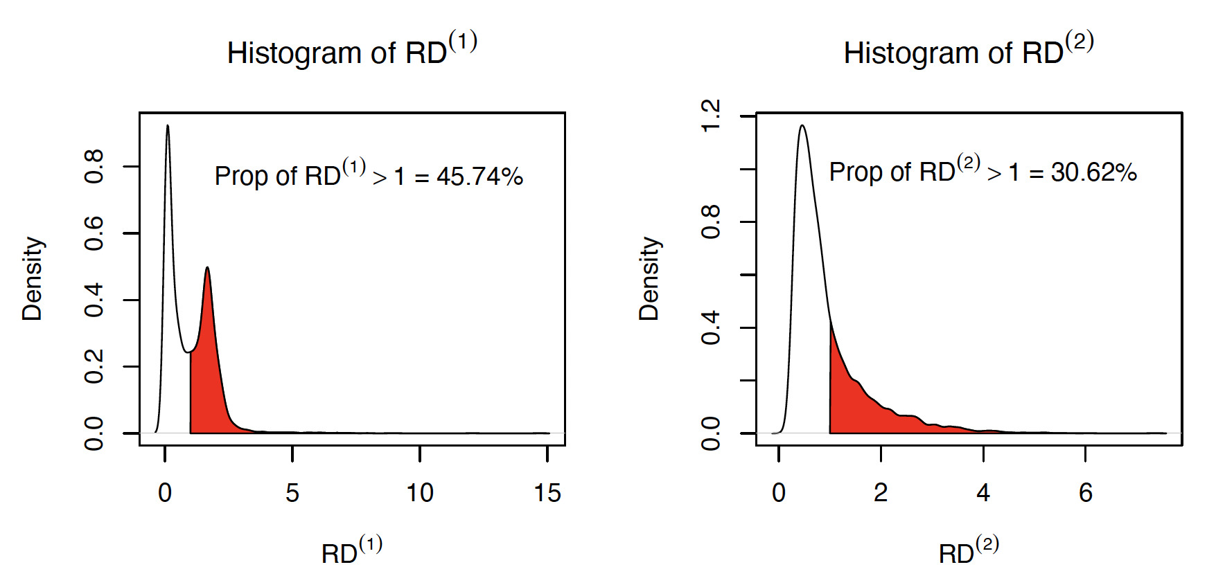
Lastly, we use the validation dataset to compare the premiums under Trad (Model 1) and TScore\(j\) (Model 3 with \(j=1\) and Model 4 with \(j=2\)). Recall that Trad (Model 1) does not use the telematics features. For that purpose, we define the relative difference of premiums between TScore\(j\) and Trad by

\[\begin{aligned} RD_i^{(j)} = \frac{\mu_i^{\text{TScore}j} } {\mu_i^{\text{Trad}}}, \quad j = 1, 2. \end{aligned}\]

Figure 3 displays the distributions of \(RD^{(1)}\) and \(RD^{(2)}\) under the validation dataset. We observe that about 46% (respectively, 31%) of policyholders will pay a higher premium if the insurer replaces Trad with TScore1 (respectively, TScore2) for ratemaking.

Figure 3.Distributions of the relative premium differences \(R D^{(1)}\) and \(R D^{(2)}\).

We conclude this section by remarking on the practical applicability of Models 3 and 4. Consider a new driver who wants to purchase a telematics insurance policy but has no “safety score” due to the lack of observed driving behavior. In this case, an insurer can accept her into its telematics portfolio by offering her an up-front discount (or treating her as in a safe group in terms of driving behavior) to attract new customers. The insurer then observes her actual driving via the telematics device or app over a certain period of time before it can determine her risk score (class). Upon renewal, the insurer uses the collected telematics information to decide whether the driver should continue to receive the premium discount. Such a practice is indeed followed by insurers in real markets, and one example is Progressive (see their telematics insurance website, https://www.progressive.com/auto/discounts/snapshot/, for full details).

4. Impact of Selection Bias on Base Premium

We show in Section 3 that both the in-sample and out-of-sample performance of the embedding models is promising. However, as already hinted in Remark 1, this might come at a cost—(favorable) selection bias; see, for instance, Cather (2020) for a recent treatment of this topic. In this section, we study the impact of favorable selection on the base premium.

To start, we partition the full dataset \(\mathcal{S}\) into two exclusive sub-datasets \(\mathcal{S}_0\) and \(\mathcal{S}_1\) as follows: for policyholders in \(\mathcal{S}_0\), both traditional and telematics features are observed, but for policyholders in \(\mathcal{S}_1\), only traditional features are recorded. We further assume that \(N_i\), the claim frequency of the policyholder \(i\), follows a Poisson distribution, \(N_i \sim \mathcal{P}(\mu_i)\), with \(\mu_i = \mathbb{E}[N_i]\). We first consider the traditional GLM in (4) with log-link function, \(\log \mu_i = \alpha + \gamma \cdot x_i\), for all policyholders \(i \in \mathcal{S}_0 \cup \mathcal{S}_1\). Denote \((\hat{\alpha}, \hat{\gamma})\) the estimates of the traditional GLM; that is, \((\hat{\alpha}, \hat{\gamma})\) solves the following optimization problem:

\[ (\hat{\alpha}, \hat{\gamma})=\underset{(\alpha, \gamma) \in \mathbb{R} \times \mathbb{R}^m}{\operatorname{argmin}} \sum_{i \in \mathcal{S}_0 \cup \mathcal{S}_1}\left(-\mu_i+\log N_i \cdot \log \mu_i\right) . \tag{9} \]

Given \(\hat{\alpha}\) from (9), we define base premium \(M\) by \(M = \exp(\hat{\alpha})\).

To better assess the impact of selection bias resulting from the embedding safety score, we group policyholders by their safety scores and consider a version of the discretized telematics score embedding model, under which the range \([0,1]\) of the safety scores \(R^{(1)}\) and \(R^{(2)}\) are divided into four groups as follows: Group 1 with \(R^{(j)}_i \in [0, q^{(j)}_{[1]})\), Group 2 with \(R^{(j)}_i \in [q^{(j)}_{[1]}, q^{(j)}_{[2]})\), Group 3 with \(R^{(j)}_i \in [q^{(j)}_{[2]}, q^{(j)}_{[3]})\), and Group 4 with \(R^{(j)}_i \in [q^{(j)}_{[3]}, 1]\), in which \(q^{(j)}_{[1]}\), \(q^{(j)}_{[2]}\), and \(q^{(j)}_{[3]}\) denote the first, second, and third quartiles, respectively, of the empirical safety scores \(R^{(j)}\) calculated using the training dataset for \(j = 1, 2\). (The empirical distributions of \(R^{(1)}\) and \(R^{(2)}\) are quite different, as seen from Figure 2, so their quartiles \(q^{(j)}_{[k]}\) are also different.) With the above grouping, we consider the discretized embedding safety score models

\[ \begin{aligned} \log \mu_i &= \hat{\alpha} + \hat{\gamma} \cdot x_i + \beta_1 \cdot \mathbb{1}_{\{R^{(j)}_i \in [0, q^{(j)}_{[1]}) \}} \\&\quad+ \beta_2 \cdot \mathbb{1}_{\{R^{(j)}_i \in [q^{(j)}_{[1]}, q^{(j)}_{[2]}) \}} \\ &\quad + \, \alpha^* + \beta_3 \cdot \mathbb{1}_{\{R^{(j)}_i \in [q^{(j)}_{[2]}, q^{(j)}_{[3]}) \}} \\&\quad+ \beta_4 \cdot \mathbb{1}_{\{R^{(j)}_i \in [q^{(j)}_{[3]}, 1] \}}, \end{aligned}\tag{10} \]

for \(i \in \mathcal{S}_0\) and \(j =1,2\), in which \(\hat{\alpha}\) and \(\hat{\gamma}\) are obtained from (9), and the parameters satisfy

\[\beta_4 \leq \beta_3 \leq \beta_2 \leq \beta_1=0.\]

The above constraint implies that if a policyholder belongs to a safer safety score band, she should expect a bigger discount on the premium. Because the larger the safety score, the lower the riskiness of a policy, Group 4 is the most preferred and Group 1 the least preferred to the insurer. As Group 1 is the least preferred, there shall be no discount applied to that group as implied in \(\beta_1=0\). Lastly, \(\alpha^*\) accounts for the different mean risk level between \(\mathcal{S}_0\) and the full dataset \(\mathcal{S}\), which is the so-called market segmentation effect. If we can observe the telematics features from all policyholders so that \(\mathcal{S}_0=\mathcal{S}\), then by definition \(\alpha^*=0\).

The models proposed in (10) allow us to easily analyze the realized relativities due to the (observed) safety score computed from the telematics features of a policyholder in \(\mathcal{S}_0\). Indeed, given the \(\beta\)s from (10), we define the relativity of policyholders in Group \(m\), compared to the base premium due to their safety score, by

\[\begin{aligned} RL_m = \exp \big(\beta_m + \, \alpha^*), \quad m = 1, 2, 3, 4. \end{aligned}\tag{11}\]

Since the degree of favorable selection can be modeled by the split of \(\mathcal{S}_0\) and \(\mathcal{S}_1\), we consider diverse selection schemes for traditional and telematics policies and study the corresponding changes in the implied relativities \(RL_1, RL_2, RL_3\), and \(RL_4\) due to the telematics safety score.

Assume that the sampling probability of a policy with claim frequency \(N_i\) in \(\mathcal{S}_0\) (the dataset with both the traditional and telematics features) is given by

\[\begin{aligned} p_i = \frac{1}{1+ \exp(k \cdot N_i / 6 )} , \end{aligned}\]

in which \(k\) is a parameter controlling the degree of favorable selection.^[2] The larger the value of \(k\), the stronger the favorable selection. To see this, consider \(N_i=0, k=7\) and \(N_i=3, k=7\); we compute \(p_i(N_i=0, k=7) = 0.5\) and \(p_i(N_i=3, k=7) = \frac{1}{1+\exp(3.5)} \simeq 0.029\), so policies with three claims are much less likely to appear in the telematics dataset \(\mathcal{S}_0\) than the policies with no claim. We consider various levels of \(k\), ranging from \(0\) to \(7\). Note that \(k = 0\) corresponds to the random selection scheme, since \(p_i = 0.5\) for all \(i\), while \(k=7\) represents an extreme scenario of favorable selection. We compute the relativities, defined by (11), for the four groups based on the telematics safety scores, and present the results in Figure 4. The key findings are summarized below.

Figure 4.Relativities \(R L\) in (11) for the four safety score groups under different \(k\).

• When there is no selection bias (\(k = 0\)), and thus \(\mathcal{S}_0\) is a random sample of the population (that is, \(\mathcal{S}_0\) has the same distribution as the population of all policyholders), the two proposed models, TScore1 (Model 3) and TScore2 (Model 4), can lead to higher relative premiums for some groups. For example, if the safety score is calculated by \(R^{(1)}\), both Groups 1 and 2 have relativities greater than 1, so policyholders in those groups experience premium surcharges. This result is not surprising because there is an implicit increase in the base premium for the telematics policies, implied by the difference in the estimated values of \(\alpha\) parameter between Trad (–0.4331) and the TScore1/TScore2 models (2.6114 and 1.0082, respectively) in Table 1.

• As the degree of favorable selection increases (\(k\) increases), the base premium for the telematics policies in Groups 1 and 2 decreases significantly but remains relatively stable for Groups 3 and 4; this observation applies to both \(R^{(1)}\) and \(R^{(2)}\). In the extreme case of \(k = 7\), the telematics policies in Groups 2 through 4 when \(R = R^{(1)}\) (respectively, all groups when \(R = R^{(2)}\)) in the telematics dataset \(\mathcal{S}_0\) receive a premium discount compared with those with only the traditional features. This result shows that the discount-only regulatory requirement could work as intended if there is a strong favorable selection (policyholders with good claim history are more attracted to the telematics policies).

5. Conclusion

The rapid growth of telematics insurance in recent years poses new challenges and concerns in the areas of policyholder privacy, use of telematics data, and fairness/discrimination in pricing, among others. Such concerns will necessarily compel regulators to implement new laws or policies regulating the insurance industry’s collection and use of telematics data. As a prime example, legislators in the state of New York introduced Assembly Bill 2023-A7614 in the 2023–2024 session, which contained a provision to prohibit the increase of premiums based on telematics data in the current policy year, which we term a “discount-only” regulatory requirement. The essential goal of this paper is to propose a ratemaking framework for claim frequency that, on the one hand, utilizes the available telematics features and, on the other hand, complies with such a discount-only regulatory requirement. To that end, we combine the powerful FFN with a standard GLM to build modified GLMs via a two-step approach. We first apply an FNN to transform the telematics features into a one-dimensional safety score, referred to as risk embedding, and next use it along with the traditional features in GLMs. In a second step, we impose appropriate constraints on the safety score and its regression coefficient in the GLMs to satisfy the discount-only regulatory requirement. We show that for a suitable choice of risk embedding, the proposed models can outperform standard GLMs (with or without the use of telematics features) in both in-sample goodness of fit and out-of-sample prediction. We also study the impact of selection bias (i.e., good drivers are more likely to enroll in telematics policies than bad drivers) on the base premium. Our results confirm that the discount-only constraint may force insurers to increase the base premium to compensate for the loss of revenue due to the relativity cap. However, this unwanted effect is largely alleviated in the presence of a sufficient level of favorable selection. Lastly, the safety scores we construct also have the potential to help reduce the industry’s reliance on some of the controversial traditional covariates (such as age and gender) in ratemaking practices, which aligns with recent findings in Ayuso, Guillen, and Pérez-Marín (2016) and Boucher and Pigeon (2024).

Acknowledgments

We thank two anonymous reviewers for their valuable comments on an earlier version of the paper. This project was funded by a Casualty Actuarial Society 2024 individual research grant. The first two authors were also partially supported by a Natural Sciences and Engineering Research Council of Canada grant (R832535).