Comparing Predictive Models for Dependent Risk Pricing

1. Introduction

Many common property and casualty (P&C) insurance policies, as well as health insurance policies, bundle diverse coverages in a single contract. For example, motor third-party liability (MTPL) insurance covers, in most jurisdictions, property damage to third-party vehicles and other property and bodily injuries. Similarly, health insurance may cover expenses for several medical costs and expenses, such as specialist visits, drugs, and hospitalizations. Thus, the pure (risk) premium charged by the insurer can be seen as the sum of the premiums relating to each distinct cover, where these premiums for the distinct coverages will differ by the rating structure of each coverage applied to the same policyholder.

In current actuarial practice, each cover is commonly rated on a totally separate basis, without considering any dependencies among risks. In other words, the pricing models for each cover are built with reference only to the experience on each distinct coverage. In practice, for those covers with fewer claims due, for example, to the rating profile, it is harder to build robust predictive models for rating purposes. From an academic perspective, improving this situation with new approaches has been considered by several authors. One approach, taken by Frees, Shi, and Valdez (2009), considered integrating copulas within a classical generalized linear model (GLM) framework (see Goldburd, Khare, and Tevet [2016] for a standard reference on GLMs). Meanwhile, the past decade has seen the rise of various machine learning (ML) techniques. The most notable of these from the perspective of P&C pricing are gradient-boosted trees (GBTs) and deep learning (DL), with which P&C pricing actuaries are becoming increasingly familiar. Successful actuarial applications of ML techniques range from mortality modeling to claims reserving, ratemaking, policyholder’s behavior, and telematics (Richman 2021a; Spedicato, Dutang, and Petrini 2018). Schelldorfer and Wüthrich (2019) shows an empirical application of DL architectures for actuarial pricing. DL architecture can naturally model multidimensional outcomes jointly, such as the frequency and the severity of distinct perils. A part of the network structure would be shared, ideally extracting hidden features that impact all outcomes, while the final branches would specialize on peril-specific modeling. Thus, DL models should—in theory—offer more robust estimates of the pure premium than those obtained by separately modeling each peril. Finally, since the last part of the 2010s, the transformer architecture has allowed DL models to reach state of the art (SOTA) performance in natural language processing (NLP) and computer vision (CV) tasks (Vaswani et al. 2023) and has been successfully applied in actuarial pricing as well (Richman, Scognamiglio, and Wüthrich 2024).

The main aim of this paper is to explore the potential of DL-based models in multiperil risk pricing, when not only the risk components (the frequency and the severity) but also the distinct covers bundled in the policy are modeled together. This approach, little explored at the time of writing this paper, will be compared with the “traditional” independent modeling approach to building models, whether for frequency and severity separately or for different covers independently. The rationale for our approach is that these models will likely be able to successfully capture the dependencies among the distinct covers, leading to better predictive performance and more robust estimates of the pure premium.

We will demonstrate our proposed framework on several real actuarial datasets. After a brief literature review on multiperil modeling, we will describe the proposed model. The empirical part of the paper will set out the general framework that we employ, explaining the modeling choices and comparing the predictive performance of GBT, multilayer perceptron deep learning (MLP), and transformer-based deep learning (TRF) models. Considerations regarding the interpretation of the models and computational issues will be considered as well.

The rest of this manuscript is organized as follows: Section 2 provides a comprehensive literature review, covering both the theoretical foundations of multiperil pricing and recent developments in ML applications within actuarial science. Section 3 presents an overview of the ML methods compared in this study, including GBT, MLP, and TRF architectures. Section 4 details our proposed modeling framework for joint multiperil pricing and describes the dataset used in our empirical study. Section 5 presents the results of our comparative analysis, including model performance metrics, interpretation of key findings, and computational considerations. Finally, Section 6 concludes with a discussion of the implications for actuarial practice and outlines promising directions for future research in this domain.

2. Literature review

2.1. Multiple outcomes pricing

Actuarial practitioners typically use separate predictive models when pricing insurance policies that cover multiple risks. These models are independently applied to estimate both claim frequency and average claim severity for each coverage type, operating under the assumption that frequency and severity are independent components, and that risks associated with different types of coverage are also independent of one another. However, the limitations of this approach have been widely recognized in literature. Over the past decade, several studies have explored alternative methodologies, addressing the assumption of independence between claim frequency and average claim severity within the same insurance coverage. Garrido, Genest, and Schulz (2016) proposed a methodology to relax the assumption of independence between frequency and severity within the GLM framework. Their approach incorporates the modeled number of claims as a covariate in the severity model, directly linking these two components. This concept is further extended in the work of K. Shi and Shi (2024), which, at the time of drafting this document, is the only study in the actuarial literature to apply DL to jointly model frequency and severity. Its framework uses a deep neural network to model frequency, with the predicted output subsequently serving as an input to model conditional severity. Additionally, the approach integrates LASSO regularization to manage parameter sparsity and enhance the interpretation of the proposed model. Another approach that has been explored is to model pure premium (in other words, the combination of frequency and severity) as a single outcome, using models with a Tweedie loss distribution. P. Shi and Zhao (2020) show that the Tweedie regression can be viewed as the independence limit of the more general copula-compound model, which, by contrast, enables explicit modeling and estimation of dependencies between claim frequency and severity. Conversely, Delong, Lindholm, and Wüthrich (2021) concludes that modeling pure premium with a Tweedie approach does not result in greater predictive accuracy.

The idea of joint modeling of multiple insurance covers simultaneously has not been explored in great depth in the actuarial literature; a brief review on the topic follows. Frees, Shi, and Valdez (2009), Frees, Meyers, and Cummings (2010), and L. Yang and Shi (2019) represent notable examples of the modeling approach that has been consolidated in the actuarial literature. In general, these studies use multivariate parametric regression models, often belonging to the GLM family, to relate the risk components to the ratemaking factors; copulas are used (except in one paper) to model the dependencies across perils. Some details about the papers reviewed follow.

Equation 1 expresses the likelihood of the model proposed by Frees, Shi, and Valdez (2009). The rightmost term in Equation 1 is the severity component, while the leftmost term relates to the frequency. The frequency component integrates individual-peril multivariate logistic regressions and pairwise-perils dependency ratios that represent the ratio of joint claim occurrence probability to the product of the individual claim occurrence probabilities (the independence assumption). The severity component is modeled using a multivariate gamma distribution, with the copula function modeling the dependencies across perils.

\[ \begin{align} l_{i}\mspace{6mu} &= \mspace{6mu}\sum_{j = 1}^{c}\ln f\left( y_{ij},\,\theta_{ij},\,\text{scale}_{j} \right)\mspace{6mu} \\&\quad+ \mspace{6mu}\ln\left\lbrack {cop}_{N}\left( F_{i1},\ldots,F_{ic} \right) \right\rbrack \end{align} \tag{1} \]

\[ \tau_{12}\mspace{6mu} = \mspace{6mu}\frac{\pi_{12}}{\pi_{1}\,\pi_{2}}\mspace{6mu} = \mspace{6mu}\frac{\Pr\left( r_{1} = r_{2} = 1 \right)}{\Pr\left( r_{1} = 1 \right)\,\Pr\left( r_{2} = 1 \right)} \tag{2} \]

The out-of-sample validation of the approach on a large homeowners insurance portfolio suggests superior predictive performance of the proposed model.

Frees, Meyers, and Cummings (2010) uses a hierarchical approach to model the loss cost of a Singapore MTPL portfolio that covers three kinds of perils. Equation 3 expresses the structure of its model: the joint distribution of the number of claims \(N\), the type of claims \(M\), and their loss cost \(y\) depends on a product of three terms, each of which is a function of the ratemaking factors \(f(N)\), \(f(M \mid N)\), and \(f(y \mid N,M)\). The first term models the frequency of claims (using a negative binomial regression), the second term models the type of claims (i.e., which combination of claims occurs) using a multinomial regression, and the third term models the severity given the number of claims (where a generalized beta of the second kind is used, GB2). A t-copula allows for marginal dependencies across the severities.

\[ f(N,M,y) = f(N)\, \times \, f(M \mid N)\, \times \, f(y \mid N,M) \tag{3} \]

The authors apply their parametric framework to simulate the predictive distribution of individual risk ratings and the impact of various policy forms (varying deductibles and policy limits) as well as to evaluate different risk metrics (such as value at risk and conditional tail expectation) and the impact of reinsurance.

Equation 4 is the key equation of the L. Yang and Shi (2019) approach that rates multiple perils on a longitudinal. The vector \(\eta_{j} = \left( \eta_{j}^{F},\eta_{j}^{S} \right)\) contains the parameters of the frequency and severity components, respectively, of the peril \(j\) at time \(t\) for the policyholder \(i\). The two-part models allow for the zero-mass distribution of the loss cost modeling the probability of no-claim occurrence in frequency term, while a GB2 regression models the cost component. Finally, a Gaussian copula is used to model the cross-sectional dependence among perils, the serial correlation among the longitudinal outcomes, and their interaction.

\[\begin{align} F_{it,j}(y) &= F_{j}\left( y;\, x_{it,j},\eta_{j} \right) = Pr\left( Y_{it,j} \leq y \mid x_{it,j} \right) \\&= p_{j}\left( x_{it,j},\eta_{j}^{F} \right) \\&\quad+ \left( 1 - p_{j}\left( x_{it,j},\eta_{j}^{F} \right) \right)\, G_{j}\left( y;\, x_{it,j},\eta_{j}^{S} \right) \end{align} \tag{4} \]

The model proposed in the L. Yang and Shi (2019) paper expresses superior fit in terms of log-likelihood-based metrics and out-of-sample predictive performance compared to the independent modeling approach.

2.2. ML in the insurance industry

A recent survey on the European market indicates that ML techniques other than GLMs are mostly applied in fraud prevention, claims management, and churn modeling in the insurance industry. Methods based on decision trees (e.g., GBT) are the most used approaches (Vergati, Rositano, and Laurenza 2023), followed by DL for specialty applications. A comprehensive review of scholarly applications of DL in actuarial science can be found in Richman (2021a, 2021b).

GLMs, introduced in the 1990s, are still the reference approach in actuarial pricing in practice (Goldburd, Khare, and Tevet 2016). Their current use within practical applications may leverage newer techniques, such as generalized additive models (GAMs) (Klein et al. 2014) for handling continuous covariates (as opposed to binning these, which is a practical alternative that has often been used). Beyond GLMs, the past decade has seen a dramatically rising interest in applying ML model applications within actuarial pricing. Henckaerts et al. (2021) presents a complete application of GBT models in actuarial pricing. ML models have not only been proposed as a standalone approach but also as a reinforcement of traditional GLM approaches. Henckaerts et al. (2018) shows how decision trees and clustering approaches can be used to group the GLM scores from high-cardinality categorical covariates and GAM marginal effects to obtain simple binning of variables entering a GLM, leading to a simpler and more interpretable tariff structure with improved predictive power. A review of the main ML models for modeling the number of claims (GLM, GBT, and MLP) is offered by Noll, Salzmann, and Wüthrich (2020). Another approach is the combined actuarial neural network (CANN), which combines the input of a traditional GLM with contributions by an MLP model into a final prediction; this has shown more competitive results than GLM, GBT, and MLP models used as standalone approaches (Schelldorfer and Wüthrich 2019). The recent TRF-based architectures, which have achieved tremendous success in NLP, have also recently been applied to actuarial contexts. Specifically, Brauer (2024) presents a review of the application of TRF models in actuarial pricing, producing improved results over more generic DL methods. Along these lines, recent work by Richman, Scognamiglio, and Wüthrich (2024) has introduced a novel credibility transformer that combines TRF architectures with principles from credibility theory, showing that even SOTA TRF models can be improved using classical actuarial credibility principles.

2.3. Our proposed contribution in the context of multiple risk pricing

The methodologies proposed in our paper leverage ML techniques, both when independently modeling frequencies and average severities for each individual coverage, and when jointly capturing dependencies across multiple covers. These approaches are inherently nonparametric and exhibit intrinsic nonlinear flexibility compared to traditional multivariate regression models. Both the MLP and the TRF architectures initially process inputs jointly through shared network layers, before branching into specialized output layers tailored to individual targets. As further detailed in the paper, the TRF architecture leverages the “attention mechanism” that dynamically weighs the importance of each covariate relative to the others in the context of multiple outcomes. This enables the network to extract and synthesize interactions among features, refining target-specific predictions by explicitly modeling cross-target relationships.

3. Overview of ML methods for non-life pricing

This section provides a brief theoretical review of the three methods—GBT, MLP, and TRF—that will be applied in our study. As a general remark, numerical outcomes in the form of claim counts will be assumed to be Poisson distributed, i.e., \(N_{i} \sim \text{Poi}\left( \lambda\left( x_{i} \right)v_{i} \right)\), where \(v_{i}\) is an exposure measure for the i-th observation. As in most non-life pricing applications, \(v_{i}\) is the insured’s exposure to the risk, that is, the number of policy years, for example. \(\lambda\left( x_{i} \right)\) is assumed to be a function of the input predictors, \(x_{i}\). Similarly, we assume that the cost outcomes, \(X_{i}\), follow a continuous distribution, usually the gamma distribution, which can be defined by a mean \(\mu_{i}\) and dispersion parameters. As we did for frequency, we assume that the mean parameter \(\mu_{i}\) of the risk component is a function of the input predictors, \(x_{i}\), such that \(\mu_{i} = g\left( x_{i} \right)\).

3.1. Boosting algorithms

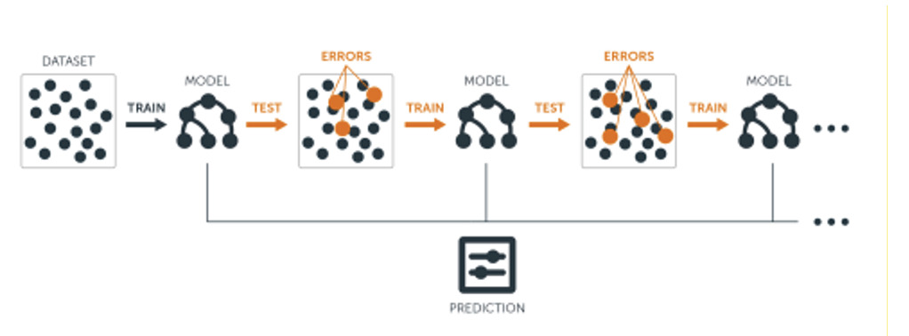
Boosting algorithms belong to the family of ensemble methods and have proven their effectiveness in a wide range of classification and regression problems. The core idea can be expressed by Equation 5:

\[ F_{t}\left( x_{i} \right) = F_{t - 1}\left( x_{i} \right) + \lambda\, f_{t}\left( x_{i} \right) \tag{5} \]

where the prediction at the \(t\)-th step is the prediction from the previous step plus the contribution of a “weak learner” \(f_{t}\), which attempts to correct the prediction errors from step \(t - 1\), weighted by a factor \(\lambda\) (often referred to as the learning rate or shrinkage factor). At each iteration, observations are re-weighted based on their prediction error from the previous step, giving more importance to poorly predicted samples. A common choice for \(f_{t}\) is a relatively simple example of classification and regression trees (CART), which, when combined into an ensemble, are highly effective at approximating functions.

Using the notations introduced by Ferrario and Hämmerli (2019), the boosting algorithm seeks to minimize the objective expressed by Equation 6:

\[ \mathcal{L}(F): = - \frac{1}{n}\sum_{i = 1}^{n}L\left( Y_{i},F\left( x_{i} \right) \right),\quad F\mathcal{\in F} \tag{6} \]

where \(L\) is the loss function that quantifies the error of predicting the target \(Y_{i}\) with \(F\left( x_{i} \right)\). Typical loss functions include quadratic loss, logistic loss, and exponential loss. The function \(F\) is optimized within the subspace of finite linear combinations of weak learners. Denoting each weak learner by \(f_{k}\), we have

\[F = \sum_{k = 1}^{M}\alpha_{k}f_{k}\mathcal{\in F,}\]

where \(M\) is the number of boosting iterations.

To construct this ensemble, various approaches can be used. The most successful one was proposed by Friedman in 2001 and is based on the gradient of the loss function. The basic idea is to approximate the gradient of the loss function at each iteration and to use this approximation to fit a new tree, which is then used to update the prediction. Equation 7 expresses how in gradient boosting the relationship between two consecutive iterations is determined by the additive contribution of the gradient of the loss function, weighted by the shrinkage factor (i.e., the learning rate) \(\lambda\).

\[ \mathbf{f}_{m} \rightarrow \mathbf{f}_{m + 1} = \mathbf{f}_{m} - \lambda\nabla\mathcal{L}\left( \mathbf{f}_{m} \right) \tag{7} \]

Significant implementations and advancements of boosting algorithms, listed chronologically, include AdaBoost and its variants (Freund and Schapire 1997; Hastie et al. 2009), gradient-boosting machines, and XGBoost (Chen and Guestrin 2016). The latter belongs to the GBT family, where CART are typically used as weak learners. This makes \(F_{t}\) an ensemble of trees grown by approximating a regularized objective:

\[ \mathcal{L =}\sum_{i = 1}^{n}L\left( {\widehat{y}}_{i},y_{i} \right) + \sum_{m = 1}^{M}\Omega\left( f_{m} \right), \tag{8} \]

where \(\Omega\left( f_{m} \right)\) is a regularization term that penalizes model complexity to avoid overfitting. Various regularization terms can be used, including the L1 and L2, which are commonly used in GLMs. We refer to the documentation of several different implementations of boosting algorithms for a comprehensive overview of the different regularization terms that can be used in these algorithms.

A CART partitions the portfolio into homogeneous groups of risk profiles based on specific characteristics, which are usually observable and understandable. In particular, the predictors’ space (given by the set of ratemaking factors) is partitioned into \(J\) nonoverlapping regions \(R_{1},R_{2},\ldots,R_{J}\) such that \(f_{\text{tree}}\left( \mathbf{x} \right) = \sum_{j = 1}^{J}{\widehat{y}}_{R_{j}}\mathbb{1}\left( \mathbf{x} \in R_{j} \right)\) where \({\widehat{y}}_{R_{j}}\) is the expected value of the risk indicator (i.e., the frequency or the severity) in the \(R_{j}\) partition. Ensembles of trees exhibit an interesting trade-off. The predictive performance of a single tree is generally quite low, but a single tree is usually quite interpretable. An ensemble of trees usually has excellent predictive performance, but, due to the aggregation of many trees, the ensemble itself becomes quite complex and hard to interpret.

Figure 1.An illustration of a GBT model structure.

As previously explained, in a GBT each weak CART improves the current fit contributed by the previous trees. At each iteration “pseudo-residuals,” calculated as the negative gradient of the loss function weighted by the shrinkage parameter—which are evaluated at the current predictions from the ensemble—are modeled to improve the fit in the direction of a better performance in regions where the current model performs poorly.

Boosting algorithms can be adapted to problems traditionally addressed by GLMs, such as logistic, Poisson, and gamma regressions. A key feature shared with GLMs in actuarial modeling is the ability to initialize predictions with a specified offset, as in rate modeling with Poisson regression, as discussed in Yan et al. (2009). Furthermore, boosting implementations also support monotonic constraints, another characteristic commonly employed in actuarial GLMs, allowing users to enforce monotonic relationships between predictors and the target variable, ensuring ease of interpretation and alignment with domain-specific knowledge. Moreover, they provide a measure of variable importance that generalizes the approach proposed by Breiman (2017). Finally, another significant advantage of GBT models is their ability to handle categorical variables and missing values with minimal preprocessing.

GBT models are defined by a set of hyperparameters that influence both the structure of the trees (i.e., maximum depth or minimum number of observations in each terminal node) and the learning process (i.e., the learning rate \(\rho\) , the fraction of predictor considered, or the fraction of observation considered). Optimal hyperparameter values can be identified through grid search or more advanced techniques like Bayesian optimization.

A comprehensive introduction and application of GBT in actuarial pricing can be found in Henckaerts et al. (2021) and Ferrario and Hämmerli (2019), while Y. Yang, Qian, and Zou (2018) presents an application of Tweedie GBT in insurance pricing.

3.2. MLP DL

A review of DL models for actuarial pricing is offered, for example, in Ferrario, Noll, and Wüthrich (2020) and Holvoet et al. (2023); here we provide a relatively brief overview of the main characteristics of these models.

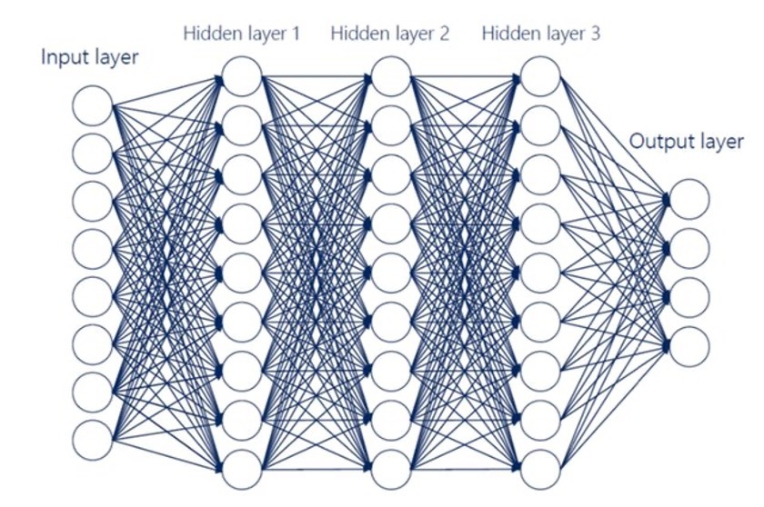
Feedforward networks (FFNs), also known as MLP neural networks, are ML models composed of a sequence of interconnected layers, \(z^{(m)}\), with \(m = 0,1,\ldots,M\). The input layer \(z^{0}\) processes the (potentially multivariate) input data, while the output layer \(z^{M}\) produces the (possibly multivariate) outputs. Between the input and output layers, one or more intermediate (hidden) layers may exist. When multiple hidden layers are present, the model is commonly referred to as an MLP DL model. The Universal Approximation Theorem (Hornik 1991) establishes that an FFN with at least one hidden layer and a nonlinear activation function can approximate any continuous function on a compact domain to an arbitrary degree of accuracy, making it a powerful tool for modeling complex relationships. The purpose of the hidden layers is to perform feature engineering, where the input data is nonlinearly transformed to extract hidden components, known as hidden features. In an actuarial context, these features can be interpreted both as latent components that best explain risk and as an automated application of the typical manual transformations (i.e., binning, crossing in interactions) that GLM practitioners perform on the inputs actually given to the GLM fitting process. The composition mechanism of the various layers within an MLP DL model allows different inputs to enter this process at different stages of computation.

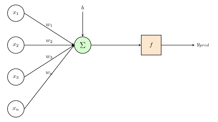
In detail, each \(k\)-th layer is composed of neurons, each one of which is connected to all the neurons of the previous layer. Each neuron applies a (non)linear transformation to the linear combination of their inputs, that Figure 2 and Equation 9 illustrate.

\[ z_{j}^{(k)}\left( \mathbf{z} \right) = \phi\left( w_{j,0}^{(k)} + \sum_{l = 1}^{q_{k - 1}}w_{j,l}^{(k)}z_{l} \right)\overset{\text{def.}}{=}\phi\left( \mathbf{w}_{j}^{(k)},\mathbf{z} \right) \tag{9} \]

Figure 2.An illustration of a neuron in a DL model.

The parameters \(w\)—which can be divided into weights, representing regression parameters, and biases, representing intercepts in the regression context—represent the factors governing the interactions among the layers. These parameters are estimated during training, and the complete parameter set of a given MLP DL model is typically organized into a single large parameter matrix \(W\).

Estimating \(W\) involves minimizing a loss function that quantifies the discrepancy between the fitted and actual data. This is achieved using the back-propagation algorithm (Rumelhart, Hinton, and Williams 1986) in combination with gradient decent methods (GDMs). The GDM begins with an initial random assignment of the \(W\) matrix and iteratively updates the parameters by taking small steps (determined by the “learning rate”) in the direction of the negative gradient of the loss, i.e., to minimize the loss function. Training proceeds over multiple passes through the dataset (epochs), during which the parameters are updated several times per epoch by processing smaller subsets of data (batches). The process continues until a predefined stopping criterion is met. Numerous variants of GDM exist, each employing different strategies to enhance convergence. Notable examples include Adam (Kingma and Ba 2017) and RMSprop (Hinton, Srivastava, and Swersky 2012). When the model has multiple outputs, the overall loss is computed as the sum of the individual losses associated with each output neuron.

The number of layers \(Q\) and the number of neurons within each layer are hyperparameters of the network, as well as the (nonlinear) activation function chosen—the hyperbolic tangent function \(\tanh(x)\) or the ReLu function \(\text{ReLU}(x) = max(0,x)\) being notable examples. Defining an MLP model thus implies making several decisions involving, for example: the loss function and performance measures, the number of hidden layers \(K\) and the neurons on the hidden layers \(q_{k}\), the activation function \(\phi\), and the optimization algorithm and its learning rate. Also, several choices to avoid overfitting exist, such as ridge and LASSO regularizers, which control the magnitudes within the weight estimation, as well as other options like normalization, dropout rates, and early stopping.

All data fed in the input layer must be numeric. To ensure that the optimization algorithm converges, numeric input needs to be preprocessed using transformations like normalization or standardization. For categorical data that commonly occur in actuarial pricing exercises, two main approaches can be used to transform these categorical covariates into numerical ones: hot encoding, which involves creating \(J\) binary variables, one for each level of a categorical variable, or so-called categorical entity embeddings—see Richman (2021a) for a detailed introduction to this approach. The variable embedding approach, which is a unique capability of MLP models, maps each level of the categorical variable into a low dimensional space (the target dimension can be chosen heuristically as the fourth root of the number of distinct categories), allowing the model to flexibly represent relations between the levels of the predictor.

Figure 3.An MLP multioutput DL model.

In recent years, DL has increasingly been applied to actuarial pricing topics. Table 1 in Holvoet, Antonio, and Henckaerts (2025) provides a comprehensive summary of the SOTA as of 2025, offering a comparative analysis of various studies that have employed DL models. This table highlights critical aspects such as the handling of categorical variables, the datasets utilized, and the alternative models benchmarked to assess predictive performance. Holvoet, Antonio, and Henckaerts (2025) applies DL models separately to claim frequency and average cost, providing detailed insights into hyperparameter selection, predictive performance comparison, and their managerial application. When evaluating the performance of DL models, it is very important to consider both the average predictive performance of several runs of these models and the predictive performance of ensembling the results of these models together; the latter is a characteristic that is not shared by traditional GLMs. For more details on this, see Richman and Wüthrich (2020). A nice feature of the DL approach to allowing inputs into the model at various levels is the explicit management of exposure in modeling claim counts when the exposure to risk varies across units. Exposure, after a log-transformation, can be introduced in a final layer that combines it with the preprocessed ratemaking factors; after exponentiating, this creates a multiplicative model on the right scale for prediction. Another similar approach has been proposed in the already mentioned CANN, where the prediction of a standard model, such as a GLM, is integrated via a “skip-connection” layer into the DL feature extraction process to produce a combined prediction, as Equation 10 displays. Holvoet, Antonio, and Henckaerts (2025) showed that, in many datasets, a CANN with GBT outperforms a standalone GBT, GLM, or MLP approach.

\[ \widehat{y} = exp\left( w_{\text{NN}} \cdot {\widehat{y}}^{\text{NN}} + w_{\text{IN}} \cdot ln\left( {\widehat{y}}^{\text{IN}} \right) + b \right) \tag{10} \]

Alternatively, as we will propose in this paper, a DL model can be designed to predict multiple outputs, such as frequency and severity, using a tree-like structure: a shared section extracts “deep features” common to both components, while separate branches perform fine-tuning for the specific outcomes.

3.2.1. Focus on categorical variables

As we have mentioned above, the management of categorical variables in neural networks for non-life pricing is a key concern, due to the significant importance of these in rating models. A categorical variable can have \(L\) distinct levels, known as its “vocabulary,” each associated with a specific frequency. A straightforward approach to bringing these into DL models is to apply one-hot encoding. However, unless the levels have relatively balanced frequencies and a low cardinality, this method results in a significant increase in dimensionality and produces very sparse vectors for each level. This can lead to instability in parameter estimation, particularly when \(L\) is large. P. Shi and Shi (2023) applies categorical auto-encoders in actuarial pricing to construct rating classes, to perform tail dependence risk analysis, and to apply transfer learning, while an extension of embedding modeling for hierarchical covariates can be found in Wilsens, Antonio, and Claeskens (2024).

An alternative approach is the use of categorical entity embeddings, introduced into the actuarial literature by Richman (2021a), which map the distinct levels of a categorical variable into a lower-dimensional metric space as shown in Equation 11:

\[ e_{t}^{\text{EE}}:\{ a_{1},\ldots,a_{n_{t}}\} \rightarrow \mathbb{R}^{b},\quad x_{t} \mapsto e_{t}^{\text{EE}}\left( x_{t} \right) \tag{11} \]

The dimension of this embedding space is typically orders of magnitude smaller than \(L\)—for example, the cube root or less of \(L\). This mapping allows the embeddings to represent categories in a way that captures their relationship to the target variable. Furthermore, the weights associated with the embeddings can be projected into the metric space, enabling the identification of similar relationships between categories with respect to the predicted outcome; for examples of this we refer to Richman (2021a).

Holvoet, Antonio, and Henckaerts (2025) proposes a different method that involves transforming categorical variables and their levels using an auto-encoder. Initially, categorical variables are one-hot encoded, and then an auto-encoder is applied. An auto-encoder is a type of neural network designed to reconstruct its input data after processing it through a series of latent layers with significantly reduced dimensionality, following an encoder-decoder structure. The encoding phase maps the input space into a lower-dimensional latent space, capturing nonlinear relationships among the features, while the decoding phase reconstructs the original input from the latent representations. This process effectively compresses the input data into a smaller latent space, making the auto-encoder a nonlinear extension of principal component analysis (PCA). This is based on work by Delong and Kozak (2023), who propose this strategy and test it in a non-life pricing context.

3.3. TRF DL

3.3.1. TRF models

The TRF model architecture was introduced in the seminal paper “Attention Is All You Need” (Vaswani et al. 2023). It builds on the earlier idea of alignment-based attention proposed by Bahdanau (2016) for seq2seq models but generalizes it to self-attention, where each input element (token, feature, etc.) can attend to the entire input sequence, including itself. The introduction of self-attention revolutionized DL in NLP, enabling breakthroughs such as the GPT models, and it has since been applied successfully in computer vision and tabular data.

The core idea of the TRF approach is that the model learns to focus on the most relevant parts of the input—often called “context” in NLP—through a learned weighting mechanism. Within the actuarial literature, Kuo and Richman (2021) gives an introduction to TRF in actuarial predictive modeling, demonstrating an early implementation of TRF models for tabular data. This paragraph draws inspiration from that work.

3.3.2. Embeddings for tabular data

Applying the TRF approach to tabular problems generally involves creating embeddings for all covariates (features). We have already discussed embeddings for categorical covariates above. For continuous (numerical) covariates, piecewise linear encoding has been shown to be highly successful (Gorishniy, Rubachev, and Babenko 2022). The idea is to transform each numerical column into a (d)-dimensional embedded vector. For an actuarial context, see the discussion in Richman, Scognamiglio, and Wüthrich (2024).

3.3.3. Self-attention mechanism

The self-attention mechanism is the core of the transformer. It updates each embedding based on the values of other covariates in the sequence, allowing the model to capture contextual information holistically. Mathematically, using the standard notation \((Q,K,V)\) for queries, keys, and values, the self-attention function is:

\[\begin{align} X^{*} &= \text{Attention}(Q,K,V) \\&= \text{softmax}\left( \frac{QK^{T}}{\sqrt{d}} \right)V. \end{align} \tag{12}\]

• \(Q \in \mathbb{R}^{q \times d}\) is the matrix of query vectors (transformed from the original input or embedding).
• \(K \in \mathbb{R}^{q \times d}\) is the matrix of key vectors.
• \(V \in \mathbb{R}^{q \times d}\) (sometimes written as \(X'\)) is the matrix of value vectors—these are projected from the original covariates.

The dimension \(d\) is usually the embedding size. Dividing by \(\sqrt{d}\) in the attention score \(\frac{QK^{T}}{\sqrt{d}}\) helps stabilize gradients. Then a row-wise soft-max is applied so that each row sums to 1, producing the attention weight matrix. Intuitively, each query row “attends” to all rows in \(V\) (the values), re-weighting them according to relevance.

The attention mechanism thus assigns a weight between 0 and 1 to each feature relative to the others for each query. The reweighted embeddings are then summed (or averaged), providing a context-sensitive representation, \(X^{*}\). In practical terms, each covariate “asks” for relevant information from other covariates (via its query), which “respond” through their keys, yielding a weighted combination of the values.

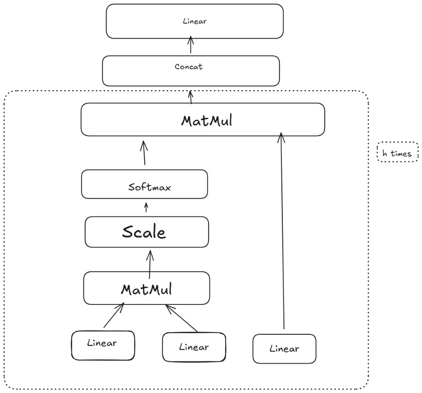
3.3.4. Multi-head attention and feedforward layers

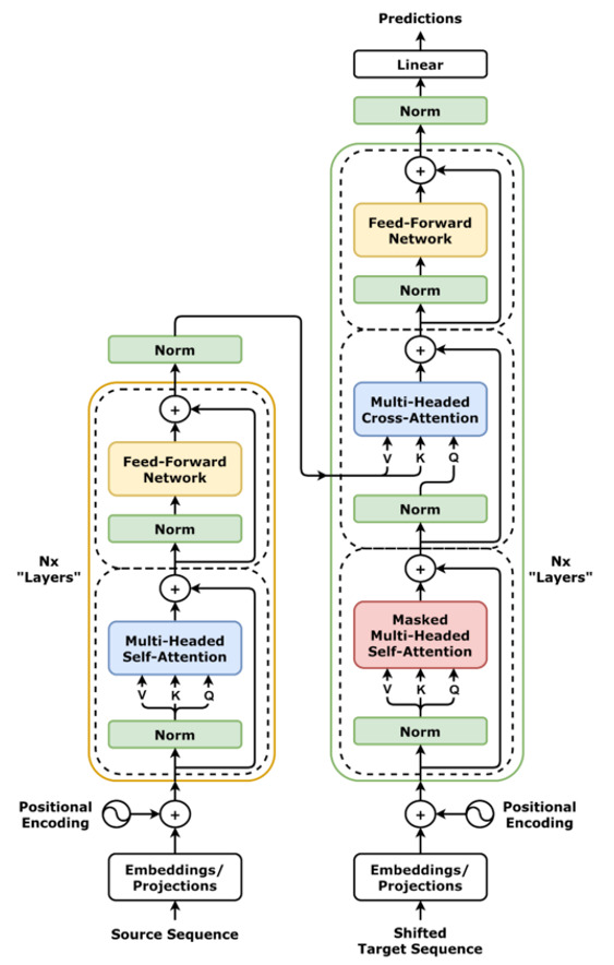
In a standard transformer, the self-attention block is followed by a feedforward sublayer, as shown in Figure 4. Additionally, multi-head attention repeats the above self-attention process \(h\) times in parallel, each with its own learnable \((Q,K,V)\) projections (with smaller dimensions). The outputs of the \(h\) heads are concatenated and linearly transformed, allowing the model to capture diverse patterns simultaneously. Multi-head attention is a key part of the TRF’s success, as it lets the model attend to multiple interaction types (or positions) at once.

Figure 4 is a conceptual illustration of multi-head self-attention.

Figure 4.Multi-head self-attention mechanism.

After multi-head attention, a feedforward layer is applied pointwise to each position (or covariate embedding) to capture nonlinear transformations. Skip (residual) connections around each sublayer allow gradients to flow more directly from outputs to inputs and reduce vanishing gradient problems. Normalization layers are also applied, ensuring stable training.

3.3.5. Positional (or feature) embeddings for tabular data

In NLP, transformer models incorporate positional embeddings (i.e., sinusoidal or learned) to indicate the order of tokens in a sequence. Tabular data, however, may not have a natural order. Accordingly:

• some approaches skip positional embeddings altogether, if feature order is irrelevant;
• others learn an embedding for each feature index (or feature name) so that the transformer “knows” which embedded vector corresponds to which original covariate.

This embedding strategy ensures that the model can distinguish between different tabular features in the self-attention layers.

3.3.6. Residual connections and final outputs

In a basic TRF model, both the original embedded covariates \((X)\) and the attention-transformed covariates \(\left( X^{*} \right)\) are combined (often by addition) to form a residual or skip connection. This technique eases optimization because the network primarily learns how to modify or refine the original inputs (learning the “delta”), rather than having to learn the full transformation from scratch. The network also includes normalization steps and a feedforward sublayer. For details in an actuarial context, see Richman, Scognamiglio, and Wüthrich (2024).

3.4. Adapting transformer models to tabular data

The original transformer architecture used in NLP tasks consists of two main modules: encoder and decoder, each typically stacked in multiple layers—six, in the original paper by Vaswani et al. (2023). In machine translation, the encoder processes the source-language tokens, and the decoder generates the target-language tokens auto-regressively. The masked self-attention in the decoder ensures the model cannot “see” future tokens.

Figure 5.A classic TRF architecture exemplified.

Since tabular applications generally involve regression or classification—where you do not need to generate a sequence of outputs one token at a time—the encoder-only variant is often sufficient. That is, the features (covariates) are embedded and processed by one or more transformer encoder layers, which produce a learned representation of each feature. A special embedding token—often called a classification (CLS) token—may be introduced to summarize all feature information into a single embedding vector for final prediction (Huang et al. 2020). In actuarial research, Richman, Scognamiglio, and Wüthrich (2024) shows how to incorporate prior information into this CLS token and combine it with the covariate information via a credibility approach.

The encoder-only approach tends to be more computationally efficient for supervised learning tasks on tabular data because there is no need for an auto-regressive (decoder) stage. Moreover, it aligns naturally with how we typically feed features into a model and obtain an output (like a single regression value or classification label).

4. Empirical application

4.1. The framework

In this study, we evaluate the predictive performance of three modeling approaches on actuarial datasets characterized by multiple coverages, where data is available for both the frequency and severity of outcomes. The models considered are GBT, MLP, and TRF. Among these, MLP and TRF belong to the broader family of DL techniques.

The GBT approach involves training separate models independently for the frequency and severity components of outcomes, with one pair of models for each coverage. This modularity allows GBT to tailor predictions specifically to each outcome type and coverage.

In contrast, the DL-based approaches, MLP and TRF, inherently model the joint distribution of frequency and severity outcomes within their architectures. These models leverage their deep structures to capture complex interactions and shared patterns across outcomes and coverages, providing a unified framework for prediction. Additionally, the study aims to investigate whether capturing potential interdependencies among risks, as well as between frequency and severity components, can improve predictive performance and to what extent this improvement is achievable. This potential improvement in the modeling of non-life and health insurance products represents a potential advantage of DL-based approaches over GBTs, which are harder to adapt to multivariate outcomes. Nonetheless, we point to the interesting work of Delong, Lindholm, and Zakrisson (2024) that provides a novel approach to doing this.

To compare the predictive capabilities of these methodologies, the three approaches will be ranked using appropriate performance metrics, separately for the frequency and severity components. In particular, given an outcome \(y_{i}\) (either the frequency or the severity), a covariate of ratemaking factors \(x_{i}\), and an exposure value \(e_{i}\) we are using the Poisson deviance Equation 13 for modeling the frequency,

\[\small{\begin{align} &D_{\text{Poisson}}\left( f\left( \mathbf{x} \right),\mathbf{y} \right) \\&= \frac{2}{n_{f}}\sum_{i = 1}^{n_{f}}\left( y_{i}\ln\frac{y_{i}}{f\left( x_{i} \right)*e_{i}} - \left( y_{i} - e_{i}*f\left( x_{i} \right) \right) \right), \end{align}} \tag{13} \]

and the gamma deviance Equation 14 for modeling the severity,

\[\begin{align} &D_{\text{gamma}}\left( f\left( \mathbf{x} \right),\mathbf{y} \right) \\&= \frac{2}{n_{s}}\sum_{i = 1}^{n_{s}}\alpha_{i}\left( \frac{y_{i} - f\left( x_{i} \right)}{f\left( x_{i} \right)} - ln\frac{y_{i}}{f\left( x_{i} \right)} \right). \end{align}\tag{14}\]

Finally, it is worth remarking that our study focuses only on modeling the expected value of the outcome, not considering the variability of such outcomes (which could be assessed by ensembling model runs together, as mentioned above) nor the uncertainty around the predicted values.

4.2. Description of the datasets

Three datasets are used in this study: a dataset of health insurance policies (HID), another representing motor third-party liability insurance policies (MTPL), and a third concerning telematic events (TLM). All three datasets include exposure, categorical and numerical covariates, and two or more outcomes representing either coverage losses or telematic events. Each outcome is described by a count variable (i.e., number of claims or events) and a corresponding column indicating the total amount or severity.

Additionally, each dataset contains a “group” column, which indicates the random assignment of each row to one of three groups: training, validation, or testing, with proportions of 70%, 10%, and 20%, respectively.

A brief descriptive summary of each dataset is provided as well as the actuarial key performance indicators (KPIs; total exposures, frequency, and severity by each outcome), while the Appendix reports the detailed tabulations of the covariates’ descriptive statistics.

4.2.1. The health insurance dataset

The HID contains data on exposures, claim counts, and their aggregate costs for a group health insurance policy that covers the following guarantees: analysis, dentistry, diagnostics, endoscopy, hospitalization, mammography, operations, and visits. Also, the following covariates are available: gender and relationship to the policyholder (categorical covariates); age at inception (numerical covariate).

Table 1 displays actuarial KPIs, while Table 10 reports descriptive statistics for its covariates.

4.2.2. The MTPL dataset

The MTPL dataset comprises data on exposures and claims for the MTPL perils covered within the Italian insurance market. In particular, “NoCard” (NC, which represents severe losses), “Card Gestionario” (CG, which represents no-fault ordinary claims) and “Card Debitore” (CD, which represents faulty ordinary claims) are reported. The interested reader may find details on the Italian MTPL statutory insurance system in IVASS (2014). NC, CG, and CD can be seen as three distinct covers that are compulsory when an Italian MTPL insurance policy is written.

Table 2 displays actuarial KPI summaries, and Table 11 reports descriptive statistics of the essential ratemaking factors provided within the dataset: vehicle and policyholder’s ages, vehicle and fuel type, calendar year, and province.

4.2.3. The telematics dataset

The TLM dataset is a table with 1,999,028 rows, providing anonymized data derived from telematics devices for automobile insurance purposes. The unique identifier of the table is the tuple “identifier_id” and “period.”

The target outcomes, “target_1” and “target_2,” represent physical phenomena recorded by the devices, in terms of both frequency and severity. Two exposure measures are available: “exposure_1” and “exposure_2.” However, our study utilized only the “exposure_1” measure.

The dataset includes covariates named with specific prefixes that indicate their domain level: “dt_” (telematic device covariates), “vhl_” (vehicle covariates), “phl_” (policyholder covariates), and “trt_” (territory covariates). Table 3 and Table 12 tabulate actuarial KPIs and descriptive statistics, respectively.

4.3. The structure of the proposed models

This section outlines the notable commonalities and specific implementation details of the three proposed approaches.

The test set, comprising 20% of each provided dataset, is used to compare the performance of the three modeling approaches using predefined metrics. A validation set, accounting for 10% of the data, is employed to prevent overfitting through an early stopping strategy. The remaining 70% of the data is allocated for training the models.

The analyses are conducted using open-source software libraries within a Python framework. The CatBoost library (Dorogush, Ershov, and Gulin 2018) is used for the GBT models, while the Keras-TensorFlow (KTF) library (Chollet et al. 2015) is employed for the MLP and TRF models. The Optuna hyperparameter optimization framework (Akiba et al. 2019) is used to tune the hyperparameters, when appropriate.

4.3.1. Gradient-boosted trees

The absolute number of claims and the average severity were modeled separately. For the models predicting the number of claims, the logarithm of the exposure was used as a base margin, serving as the starting point for the fitting process. When modeling severity, the number of claims was set as the weight. These setups closely resemble those traditionally employed when modeling such outcomes with GLMs as detailed by Yan et al. (2009).

The maximum number of trees was set relatively high (up to 5,000 for the TLM dataset and 2,000 for the MTLP and HID datasets). The final number of trees used in the fitting process was controlled by an early-stopping parameter, which monitored performance over a 50-round observation window.

The GBT implementation in CatBoost allows some hyperparameters to be set and tuned. The following list of CatBoost hyperparameters was configured and tested during the optimization process:

• learning_rate: Controls the step size at each iteration while moving toward a minimum of the loss function. Values between 0.01 and 0.1 were tested.

• depth: Specifies the depth of the tree, which impacts the model’s complexity and ability to capture patterns. Values ranged from 2 to 11.

• random_strength: Determines the strength of randomness in score calculation, which can help reduce overfitting. This varied on a logarithmic scale between 0.001 and 10.

• l2_leaf_reg: Regularization coefficient for the L2 regularization applied to leaf weights, tested over a range from 0.001 to 1 on a logarithmic scale.

• min_data_in_leaf: Specifies the minimum number of training samples required in a leaf, with values ranging from 2 to 20.

• boosting_type: Specifies the boosting strategy, either “Ordered” or “Plain.”

• bootstrap_type: Determines the method for sampling observations, with “Bayesian,” “Bernoulli,” and “MVS” options being explored.

From empirical analyses, it was observed that the final performance of the model was not particularly sensitive to the exact configuration of these hyperparameters, suggesting a degree of robustness in the model’s behavior. The Poisson loss was used to fit models for the number of claims, while root mean square error (RMSE) loss was used to fit the ones on the severity, as no native gamma loss was available within the CatBoost package at the time this paper was written.

4.3.2. MLP DL

We employed the KTF framework to design and train the MLP DL models. KTF is widely recognized in literature as the benchmark for DL models in actuarial pricing, and our model draws partial inspiration from these references (Noll, Salzmann, and Wüthrich 2020; Ferrario, Noll, and Wüthrich 2020). Several key principles guided the development of our MLP models.

DL inherently allows for the natural handling of multiple outputs, even of different types, such as claim counts and costs. This flexibility enables the hidden layers to extract both outcome-specific aspects and shared components of risk across all outcomes, thus integrating multiple perils or response variables within a single model and enhancing its applicability in actuarial contexts. As for the GBT approach, claim count outcomes were modeled by minimizing the Poisson loss, while severity outcomes minimized the RMSE.

Recent versions of KTF introduced preprocessing layers that greatly simplified the handling of numerical and categorical variables. For numerical variables, standardization was performed by the model itself. Categorical variables were either one-hot encoded or transformed into low-dimensional embeddings (using the fourth root of the cardinality of the variable) for high-cardinality features (six was judgmentally chosen as the threshold to identify high-cardinality features). The exposure measure (policy year) was handled through a dedicated input branch. The raw exposure values were retained in their original scale and subsequently log-transformed. This transformed value was added to the outcome values prior to exponentiation, ensuring the outcomes remained proportional to the exposure. These arrangements allowed us to preprocess data directly from the original dataset, improving integration and reducing the need for external preprocessing steps.

The network architecture was designed to leverage the flexibility of DL in balancing shared and outcome-specific feature extraction:

• Two or three hidden layers were shared among all outcomes to extract common “deep” hidden features.

• The network then branched into “terminal branches,” corresponding to the number of peril-specific outcomes. Each branch contained one or two additional hidden layers to extract outcome-specific features.

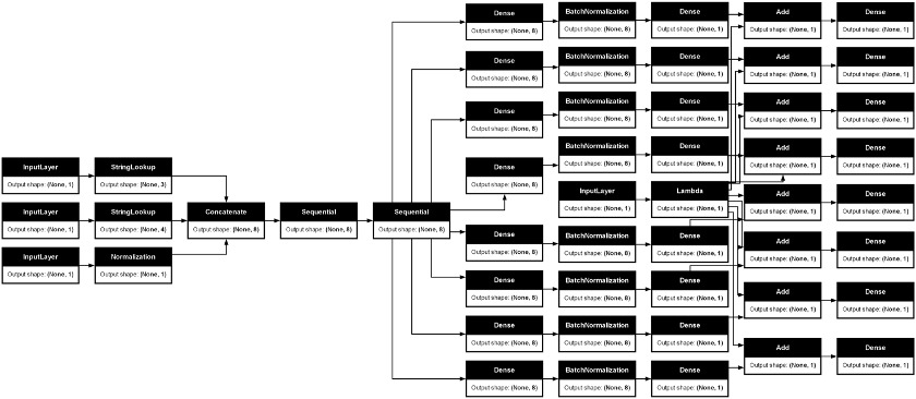
The exact configuration of hidden layers and their dimensions, as well as the application of regularization techniques (i.e., \(L2\) loss, Dropout, and BatchNormalization layers), was determined based on a combination of expert judgment and references from the literature—i.e., the work in Holvoet et al. (2023). Given the inherent difficulty in determining an optimal network structure a priori, we explored variations, with the number of shared hidden layers ranging from one to three, and similarly for the outcome-specific layers. We consistently employed the “gelu” activation function (a more recent and flexible variant of the ReLu activation) in the hidden layers (Hendrycks and Gimpel 2023), as it is well suited for modeling complex nonlinearities. Hyperparameter tuning—including layer configurations, \(L1\) and \(L2\) regularization for intermediate layers, and other parameters—was performed using the Optuna framework. The Adam optimization algorithm was used for training.

The vast combination possibilities of DL architectures, combined with the computational time required for training, means that the tested solutions represent only a small fraction of the potential configurations. It is possible that the optimal solution lies far from the tested architectures, underscoring the inherent trade-offs between practical feasibility and exhaustive exploration in DL model design.

Figure 6 displays an example of the proposed MLP DL model.

Figure 6.The MLP model exemplified.

4.3.3. Multi-target transformer architecture

This architecture addresses the problem of predicting multiple insurance targets—such as distinct perils or separate frequency-severity models—within a single framework. The principal innovation is to learn target-specific embeddings for all covariates and then incorporate a transformer layer that creates a shared representation across the multiple targets. In doing so, the model achieves a balance between allowing each target to capture its unique patterns and leveraging cross-target information that can be beneficial when different perils or coverage types share underlying risk factors.

Rational and conceptual flow

The first step is to produce target-specific embeddings of both categorical and continuous features. In many insurance applications, a given rating variable (i.e., driver age, vehicle type) can influence different lines of business or different claim components (frequency vs. severity) in distinct ways. Therefore, each target learns its own embeddings for every covariate, ensuring that the representation is specialized for that particular outcome. Mathematically, if we denote each input covariate by \(x_{j}\) and we have \(k\) target variables, we can write the embedding for target \(t\) and covariate \(j\) as

\[\mathbf{e}_{t,j} = {Emb}^{(t,j)}\left( x_{j} \right),\]

where \({Emb}^{(t,j)}\) is an embedding function (or small network) trained specifically for target \(t\). For categorical features, \({Emb}^{(t,j)}\) corresponds to a standard embedding lookup, while for continuous features a piecewise-linear transformation plus a small FFN are used to achieve the same dimensionality. This design lets each target “see” the covariates in a way that optimally suits its own predictive task—addressing, for instance, the often-different shapes of frequency vs. severity distributions.

Afterward, these target-specific embeddings are concatenated to form a single vector \(\mathbf{h}_{t}\) per target:

\[\mathbf{h}_{t} = \left\lbrack \mathbf{e}_{t,1},\mathbf{e}_{t,2},\ldots,\mathbf{e}_{t,m} \right\rbrack,\]

where \(m\) is the total number of features (both categorical and continuous). The architecture then applies a small FFN to each \(\mathbf{h}_{t}\) for an initial prediction of that target. Intuitively, this FFN captures straightforward, target-specific relationships between features and outputs. Let us define the output of the FFN for target \(t\) as

\[{\widehat{y}}_{t}^{(FFN)} = f^{(t)}\left( \mathbf{h}_{t} \right),\]

where \(f^{(t)}\) is a shallow neural module consisting of a dense layer, normalization, and dropout. The result is a preliminary estimate of the target risk metric (i.e., frequency or severity).

4.3.4. Transformer-based augmentation

While independent FFNs capture target-specific relationships, there is value in discovering cross-target interactions—the idea that certain signals in the covariates might simultaneously affect frequency and severity, or multiple lines of business. This is achieved by treating each target’s embedding vector \(\mathbf{h}_{t}\) as a token in a transformer sequence, alongside a CLS token. We can stack the target embeddings to form a matrix

\[\mathbf{H} = \begin{bmatrix} \mathbf{h}_{1} \\ \mathbf{h}_{2} \\ \vdots \\ \mathbf{h}_{k} \end{bmatrix} \in \mathbb{R}^{k \times d},\]

where \(d\) is the dimension of each concatenated embedding. In classic NLP usage, the transformer applies positional encodings to indicate the order of tokens in a sentence. Here, the model learns a positional or target-level embedding to mark which row of \(\mathbf{H}\) corresponds to which peril. A special CLS embedding vector \(\mathbf{h}_{CLS}\) is then appended:

\[\mathbf{H}' = \begin{bmatrix} \mathbf{h}_{1} \\ \mathbf{h}_{2} \\ \vdots \\ \mathbf{h}_{k} \\ \mathbf{h}_{CLS} \end{bmatrix}.\]

A multi-head self-attention module is applied to \(\mathbf{H}'\). Let us denote the resulting output sequence by

\[\mathbf{Z}' = transformer\left( \mathbf{H}' \right),\]

which has the same shape as \(\mathbf{H}'\). Because self-attention computes pairwise relevance scores among all rows, the CLS token “aggregates” cross-target information, effectively capturing which covariate signals apply similarly or differently across the various perils or lines.

CLS token for cross-target summary

Following the transformer layer, the updated CLS token \(\mathbf{z}_{CLS}\) (the last row of \(\mathbf{Z}'\)) acts as a learned summary of the entire multi-target sequence. Because attention weights allow \(\mathbf{z}_{CLS}\) to pick up signals from each target, it encodes valuable cross-target dependencies. A small FFN then transforms \(\mathbf{z}_{CLS}\) into a compact vector \(\mathbf{a}\), which is used to augment the target-specific FFN predictions. We can write:

\[\mathbf{a} = f_{CLS}\left( \mathbf{z}_{CLS} \right),\]

where \(f_{CLS}\) includes dense layers, batch normalization, and dropout. Once we obtain \(\mathbf{a}\), it is added to the concatenated FFN predictions:

\[\mathbf{p}_{aug} = \sigma\left( \mathbf{a} + \left\lbrack {\widehat{y}}_{1}^{(FFN)},\ldots,{\widehat{y}}_{k}^{(FFN)} \right\rbrack \right),\]

where \(\sigma\) is a pointwise sigmoid activation used to keep outputs in \((0,1)\). This choice of activation, while uncommon for count models, is an alternative way of ensuring a bounded “rate” parameter that can later be rescaled or multiplied by exposure for Poisson tasks. For the severity targets, we have scaled the targets to lie in \((0,1)\); we use the sigmoid here to ensure that the output of the networks is also in \((0,1)\). In some insurance contexts, this is analogous to a logit transformation but implemented via the bounded output of a sigmoid.

Final outputs for Poisson and gamma targets

Since multiple targets may have different deviance types (i.e., Poisson for frequency and gamma for severity), the final step adapts each \(\mathbf{p}_{aug,t}\) according to the target’s distribution. For a Poisson target, the model multiplies the rate \(\mathbf{p}_{aug,t}\) by the exposure \(E\), yielding predicted counts:

\[{\widehat{y}}_{t} = \mathbf{p}_{aug,t} \times E.\]

For a gamma target, which might represent severity, the output remains \(\mathbf{p}_{aug,t}\), or it can be rescaled as needed. All final outputs are concatenated into a single vector, producing a multi-output architecture that simultaneously predicts multiple perils or frequency–severity components.

We show the TRF model in Figure 7.

Figure 7.Transformer architecture for multi-target insurance modeling. The model processes each target separately through embeddings, then uses self-attention to capture cross-target dependencies via a CLS token. The final prediction combines target-specific FFNs with the learned cross-target information.

Why this works

By separating the embeddings per target, the model allows each line of business or each distribution family (frequency vs. severity) to process the same covariates in a customized manner. The transformer then introduces the crucial step of aggregating these representations so that each target can learn from shared structure in the data. This is especially relevant when numerous lines of business are correlated or when frequency and severity signals overlap in subtle ways. The CLS token distills these cross-target interactions into a single embedding that can then refine the initial predictions.

Mathematically, this approach balances “specialization” and “collaboration.” Specialization occurs as each target gets its own embedding \(\mathbf{e}_{t,j}\), while collaboration arises through self-attention across the entire matrix \(\mathbf{H}\). The final additive step combines the two worlds: localized predictions (via the FFN) plus cross-target knowledge (via the transformer’s CLS). In insurance pricing or loss-cost modeling, such synergy can lead to more robust estimates, particularly in the presence of limited data for certain coverages or subpopulations.

Practical implementation details

In practice, the architecture can be trained end-to-end using standard back-propagation. The piecewise-linear encodings for continuous variables were chosen heuristically, indicating that even without extensive hyperparameter tuning, the model can flexibly capture nonlinear relationships in numeric features. The embedding dimensions for categorical variables and the network widths for the transformer can be adjusted based on data size, number of features, and computational constraints.

Throughout, dropout and batch normalization mitigate overfitting and stabilize training. The final outputs for each target are kept separate (and can be reassembled) to handle different link functions: Poisson predictions require multiplication by exposure for a rate-based forecast, while a gamma target might simply interpret the raw output as severity.

Overall, this multi-target TRF architecture offers a unified approach to predictive modeling in insurance, accounting for both target-specific embeddings and cross-target shared representations, all driven by attention mechanisms that learn context at scale.

5. Performance assessment and models’ interpretation

5.1. General criteria

The following metrics were used to evaluate and rank the performance of the proposed models: The mean Poisson deviance was used when the outcome is a number of claims (see Equation 13), while the RMSE was used when the outcome is the severity, as shown in Equation 15. Clearly, only observations with a corresponding number of claims greater than zero were considered when assessing severity. RMSE was chosen as the comparison metric instead of gamma deviance, as it is more commonly used by practitioners when evaluating predictive models on continuous data—even though there is no difference in model ranking between the two approaches in our application.

\[ \text{RMSE} = \sqrt{\frac{1}{n}\sum_{i = 1}^{n}\left( y_{i} - {\widehat{y}}_{i} \right)^{2}} \tag{15} \]

In Equation 16, \(F(y)\) represents the cumulative population proportion, while \(L\left( F(y) \right)\) stands for the cumulative event proportion. The latter ranking metrics, popular for comparing competing model among actuarial practitioners (Frees, Meyers, and Cummings 2014; Lorentzen, Mayer, and Wüthrich 2022), can be used for all types of outcomes as they are nonnegative.

\[ G = 1 - 2 \times \int_{0}^{1}L\left( F(y) \right)dy \tag{16} \]

5.2. Summary of performance metrics across perils

Table 4 displays the performance metrics of the three models (CatBoost GBT, MLP, and TRF) across perils for the three datasets (ds) on the test portion. The table also shows the gamma loss, the actual/predicted ratio, and the Gini index that Equation 16 expressed. The actual/predicted ratios (ap_ratio) are in general close to 1 (with the sole exception of the NC component of the MTPL dataset), thus indicating that there is no distortion in the models—i.e., these are well calibrated. Similarly, the Gini scores are consistently distant from zero, thus indicating that the proposed models differentiate risk profiles.

When ranking the modeled performances for severity (using the gamma loss, gammaDev) and for the number of claims (using the Poisson log-loss, poiDev), we observe that the TRF approach shows the highest rank, followed by GBT, as Table 5 shows. In general, however, the loss differences between the three models are very close.

5.3. Comparison of models’ results

In this section, we perform a deeper analysis of the models, focusing on how we can interpret and compare these. We choose the TLM dataset for this purpose, as the number of output variables is relatively limited (two outcomes) and the number of data points is the greatest—i.e, the models’ fit on this dataset should be among the more stable ones in this study. Table 6 and Table 7 display the correlation of the models’ scores for the frequencies and the severities, respectively. The Spearman rank correlation measure was used to correlate score, as this metric is considered more appropriate for ranking tasks and when the variables under analysis are markedly skewed (Spearman 1987).

The tables suggest that, generally, the scores express a high level of consistency within different modeling approaches, as indicated by the positive sign and the magnitude of the correlation coefficients. Notably, the magnitude of the correlations is stronger for frequency models than for severity models. One possible explanation for this pattern is the higher relative variability inherent in average costs, which has been widely observed in many empirical studies in actuarial contexts. This intrinsic variability, coupled with the same amount of data available for the models, leaves a larger portion of unexplained variability in severity models. Furthermore, it appears that DL-based models (MLP and TRF) are more correlated with each other compared to the GBT model. Additionally, the TRF model seems to correlate more strongly with both the GBT and MLP models than the GBT and MLP models correlate with each other. One hypothesis is that the TRF model may synthesize distinct aspects that are captured separately by the GBT and MLP models, though this is speculative and warrants further investigation in future studies.

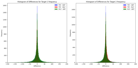
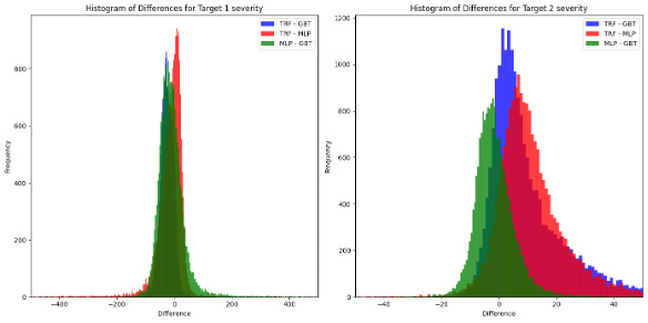
On the other hand, Figure 8 and Figure 9 display the difference between models’ pairs for the number and the claim severities, respectively.

Figure 8.Analysis of the difference within the frequency models.

Figure 9.Analysis of the difference within the severity models.

From Table 5, it was observed that all models, across all outcomes, are generally unbiased, as indicated by actual/predicted ratios being centered around 1. Among the tested models, the TRF consistently demonstrated superior performance, particularly in terms of risk discrimination ability, as evidenced by higher Gini coefficients.

When analyzing the differences between model predictions, the following patterns emerge:

1. Frequency models: The differences are well centered around zero, with no significant deviations. This indicates that the predictive behaviors of the models are highly aligned for frequency-related outcomes.

2. Severity models: Greater absolute differences are observed, particularly for Target 2 severity. However, when normalized by the average value of the outcome, these differences are reduced to approximately 1%. Notably, the TRF appears to diverge more significantly from the other models (GBT and MLP), while the difference between GBT and MLP remains symmetrically centered around zero.

3. Distribution shape and kurtosis: The distributions of differences exhibit high kurtosis, characterized by pronounced tails. This suggests a higher-than-normal presence of extreme values, which could stem from:

   • model-specific behaviors on distinct subsets of the dataset, and/or

   • the intrinsic variability of actuarial data, where outliers are expected due to the stochastic nature of claims.

These findings should be considered a preliminary hypothesis, and we cannot rule out that the observed discrepancies are merely a peculiarity of the specific dataset analyzed.

5.4. Analysis of feature importance

Both the CatBoost implementation of GBT and the novel TRF approach can be analyzed to provide measures of the variables’ importance, as Table 8 shows. Specifically, the “PredictionValuesChange” approach has been used for the GBT model (Team 2025). In the context of the TLM dataset, device-related variables appear to have a significant impact on frequency outcomes, whereas the relative importance weights are more evenly distributed among predictors for severity outcomes.

The TRF model consists of both FFNs and a transformer; we have not yet developed a method to produce variable importance measures directly from this hybrid model. Instead, we apply a surrogate model in the form of fitting CatBoost models between the variables entering the TRF model, and we use the importance metrics from the surrogate CatBoost models to help interpret the TRF model. We show this evaluation of variable importance in Table 9.

We observe that the device-related variables are by far the dominant ones in the TRF model for both frequency and severity, suggesting that the TRF model learns a relatively different set of relationships especially for the severity models, in the context of comparing these results to those for the CatBoost model just presented.

6. Conclusion and further research

Our study compared three distinct approaches for modeling the risk component of multiperil policies: the common-practice peril-independence framework using GBTs and two DL-based approaches that inherently incorporate dependencies across perils and risk components: a plain MLP and a TRF-based model. The GBT approach demonstrated strong performance, generally outperforming the MLP. However, the TRF approach consistently surpassed both the MLP and GBT approaches, even without hyperparameter tuning. This suggests that the TRF approach that has been explored in actuarial modeling—i.e., in Richman, Scognamiglio, and Wüthrich (2024)—holds significant promise not only in NLP tasks but also in multivariate risk modeling. However, the improved predictive performance comes at the cost of requiring greater expertise and higher computational resources than the other approaches. Moreover, although not applied in this study, explainable artificial intelligence (xAI) techniques are considerably more mature and well established for GBT models—e.g., the Shapley values (Lundberg and Lee 2017)—compared to DL models, which require more customized implementations that are not as widely popular as those for GBT models.

The study of interdependencies between covers and between risk components can be approached from multiple perspectives, and the models presented in this paper represent only specific implementations of these concepts, where we have tried to learn useful representations across risks and perils. These same models could be further explored, for example, through hyperparameter optimization or by investigating more innovative modeling strategies. For instance, exploring approaches based on Tweedie regression (Dunn and Smyth 2001) could be valuable, as it allows for modeling dependencies within each cover directly, i.e., without separately analyzing frequency and average cost, thereby bypassing the need to model these components individually. Another interesting direction would be to address the uncertainty of predictions from a probabilistic perspective, as was done in earlier approaches using copulas to capture joint dependencies.

In fact, future research could focus on refining these methodologies, optimizing their parameters, and exploring novel probabilistic frameworks to enhance both predictive accuracy and interpretability in multiperil risk modeling. Whereas our approach focuses on modeling the dependencies among losses in terms of expected values, correlation between residuals of predictions has not been considered in our study. While probabilistic DL has been briefly explored (Dürr, Sick, and Murina 2020), its current implementations remain computationally immature for integration into the developed framework.

Acknowledgments and disclaimers

This research was funded by the Casualty Actuarial Society (CAS), the Actuarial Foundation’s Research Committee, and the Committee on Knowledge Extension Research of the Society of Actuaries (SOA). The authors gratefully acknowledge the invaluable assistance of the CAS and SOA staff who supported this project, as well as the anonymous reviewers whose insightful feedback substantially improved the quality of the paper.

The views, analyses, and conclusions presented in this study are solely those of the authors and do not necessarily reflect the positions or policies of their employers or of the sponsoring organizations.

Repositories

To provide reproducible results, the paper materials are available in the following repositories:

1. Google Drive for dataset Google Drive folder
2. GitHub repository for code, paper, and supporting materials GitHub repo