Embeddings and Attention in Predictive Modeling

undefined

1. Introduction

Actuaries model categorical data in many different contexts, from pricing of insurance products to reserving for the liabilities generated by those products. Sometimes, these data are modeled in an explicit manner. For example, when building models that apply across multiple categories, a form of dummy coding is usually used. When building models to price the frequency of motor insurance claims, for example, the actuary will often model claim experience relating to different types of motor vehicle by including a (single) factor within models that modifies the relative frequency predicted for each type of vehicle. In other cases, modeling is performed for each category separately—thus the categorical data are used within the modeling in an implicit manner. For example, it is common practice to estimate reserves for different lines of business separately, that is to say, with no parameters being shared across each of the reserving models.

Recently, several studies of insurance problems have applied an alternative approach, originally from the natural known as categorical embeddings. Instead of trying to capture the differences between categories using a single factor, the categorical embedding approach maps each category to a low-dimensional numeric vector, which is then used in the model as a new predictor variable.

Such an approach to modeling categorical data has several advantages over more traditional treatments. Using categorical embeddings instead of traditional techniques has been shown to increase predictive accuracy of models, for example, see Richman (2018) in the context of pricing. Models incorporating categorical embeddings can be precalibrated to traditional actuarial models, increasing the speed with which these models can be calibrated and leading to models with better explainability (Wüthrich and Merz 2019). Finally, the similarity between the vectors learned for different categories can be inspected, sometimes leading to insights into the workings of models (see, for example, Kuo (2019)).

However, several open questions about the use of embeddings within actuarial work remain, which we aim to address in this study. First, hyperparameter settings for embeddings, such as the dimensions of the embedding layer and the use of regularization techniques such as dropout or normalization, that achieve optimal predictive performance have not yet been studied in detail in the actuarial literature. In this work, we aim to study how embeddings using different settings perform in the context of a large-scale predictive modeling problem and give guidance on the process that can be followed to determine this in other problems. Although neural networks have been shown to achieve excellent predictive accuracy on actuarial tasks, many actuaries still prefer to use generalized linear models (GLMs) for pricing tasks. Thus, in this paper we consider whether transferring embeddings to GLM models can achieve better performance. Finally, in the past several years a new type of neural network architecture based on attention (Vaswani et al. 2017) has been successfully used on embeddings in the field of natural language processing, and we incorporate attention-based models into our predictive modeling example to demonstrate their use for actuarial purposes.

In this work, we make use of a National Flood Insurance Program (NFIP) dataset (Federal Emergency Management Agency 2019) that provides exposure information for policies written under the NFIP, as well as the claims data relating to those exposures.

The rest of the manuscript is organized as follows. Section 2 reviews recent applications of embeddings in the actuarial literature. Section 3 provides the notation used in the paper and defines GLMs, neural networks, and related modeling concepts, including embeddings and attention. In Section 4, we provide initial models for the NFIP dataset and consider how successfully the embeddings used in the neural network model can be transferred to a GLM model of the same data and how learned embeddings can be interpreted. We focus on attention-based models in Section 5. Finally, Section 6 provides a discussion of the results of this study and considers avenues for future research.

2. Literature review

Categorical data are usually modeled within GLMs and other predictive models using indicator variables that capture the effect of each level of the category (see, for example, Section 2 in Goldburd et al. (2020)) using one of two main encoding schemes: dummy coding or one-hot encoding. Dummy coding, used in the popular R statistical software, assigns one level of the category as a baseline, for which an indicator variable is not calibrated, and assigns the rest of the levels indicator variables, thus producing estimates within the model of how the effects of each level differ from the baselines. One-hot encoding, often used in machine learning, is similar to dummy coding but assigns indicator variables to each level—in other words, it calibrates an extra indicator variable compared with dummy coding.

A different approach to modeling categorical data is credibility theory (see Bühlmann and Gisler (2005) for an overview), which, in the context of rating, can be applied to derive premiums that reflect the experience of a particular policyholder by estimating premiums as a weighted average between the premium produced using the collective experience (i.e., of all policyholders) and the premium produced using the experience of the particular policyholder. The weight used in this average is called a credibility factor and is calculated with reference to the variability of the policyholder experience relative to the variability of the group experience. In this context, the implicit categorical variable is the policyholder under consideration.

Generalized linear mixed models (GLMMs) are an extension of GLMs that are designed for modeling categorical data using a principle very similar to that of credibility theory (Klinker 2011). Instead of calibrating indicator variables for each level of the category, GLMMs estimate effects for each of these levels as a combination of the overall group mean and the experience in each level of the category.

A different approach to the problem of modeling categorical data known as embedding layers has been introduced in an actuarial context. Note that in the next section, we reflect on similarities between the conventional approaches discussed above and embedding layers. Richman (2018) reviewed the concept of embedding layers and connected the sharing of information across categories to the familiar concept of credibility theory. In that work, two applications of embedding layers were demonstrated. The first was in a property and casualty (P&C) pricing context, and it was shown that the out-of-sample accuracy of a neural network trained to predict claims frequencies on motor third-party liability was enhanced by modeling the categorical variables within this dataset using embedding layers. Second, a neural network with embedding layers was used to model all of the mortality rates in the Human Mortality Database, where the differences in population mortality across countries and the differences in mortality at different ages were modeled with embedding layers, again producing more accurate out-of-sample performance than the other models tested.

Contemporaneous with that work was the DeepTriangle model of Kuo (2019), which applied recurrent neural networks to the problem of incurred but not reported (IBNR) loss reserving to model jointly the paid and incurred losses in the NAIC Schedule P dataset. Kuo used embedding layers to capture the effect of differences in reserving delays and loss ratios for each company in the Schedule P dataset.

Many other applications of embeddings have subsequently appeared in the actuarial literature. Within mortality forecasting, Richman and Wüthrich (2019) and Perla et al. (2020) both apply embedding layers to model and forecast mortality rates on a large scale. Wüthrich and Merz (2019) discuss how embeddings can be calibrated using GLM techniques and then incorporated into a combined actuarial neural network, with subsequent contributions in P&C pricing by Schelldorfer and Wüthrich (2019) and in IBNR reserving by Gabrielli (2019) and Gabrielli et al. (2019). Other applications in IBNR reserving are found in Kuo (2020) and Delong et al. (2020), who use embedding layers to model individual claims development.

3. Theoretical overview

In this study, we are concerned with regression modeling, which is the task of predicting an unknown outcome \(y\) on the basis of information about that outcome contained in predictor variables, or features, stored in a matrix \(X\). For simplicity, we consider only the case of univariate outcomes, i.e., \(y \in \mathbb{R}^1\). The outcomes and the rows of the predictor variable matrix are indexed by \(i \in \{1 \dots I\}\), where \(i\) represents a particular observation of \((y_i, \mathbf{x}_i)\), where bold indicates that we are now dealing with a vector. The columns of the predictor variables are indexed by \(j \in \{1 \dots J\}\), where \(j\) represents a particular predictor variable, of which \(J\) have been observed; thus, we use the notation \(X_j\) to represent the \(j\)th predictor variable and \(X \in \mathbb{R}^J\). Formally, we look to build regression models that map from the predictor variables \(\mathbf{x}_i\) to the outcome \(y\) using a function \(f\) of the form

\[\mathbf{f} : \mathbb{R}^J \mapsto \mathbb{R}^1, \quad \quad \mathbf{x_i} \mapsto \mathbf f{(\mathbf{x_i})} = y.\]

In this study, we will use mainly GLMs and neural networks to approximate the function \(f(.)\).

The predictor variables that we consider here are of two types: continuous variables, taking on numerical values and represented by the matrix \(X_{num}\) with \(|J^{num}|\) columns, and categorical variables, which take on discrete values indicating one of several possible categories, represented by the matrix \(X_{cat}\) with \(|J^{cat}|\) columns, such that \(|J^{num}| + |J^{cat}| = J\).

3.1. Categorical data modeling

A categorical variable \(X_j, j \in J^{cat}\) takes as its value only one of a finite number of labels. Let the set of labels be \(\mathcal{P}^j = \{p^j_1, p^j_2,\dots, p^j_{n_{\mathcal{P}^j}} \}\), where \(n_\mathcal{P}^j = |\mathcal{P}^j|\) is the cardinality, or number of levels, in \(\mathcal{P}^j\). One-hot encoding maps each value \(x_{i,j}\) of \(X_j\) to \(n_\mathcal{P}^j\) indicator variables, which take a value of \(1\) if the label of \(x_{i,j}\) corresponds to the level of the indicator variable, and \(0\) otherwise. An example of one-hot encoding is shown in Table 1.

One-hot encoding is often used in the machine learning community, whereas the statistical community often favors dummy coding, which, instead of assigning \(n_p^j\) indicator variables, assigns one of the levels of the categories as a baseline and maps all of the other \(n_p^j -1\) variables to indicator variables. An example of dummy encoding is shown in Table 2.

After encoding the categorical data in this manner, most regression models such as GLMs will then fit coefficients for each level of the category in the table (if a tree-based model is used, such as decision tree, then splits in the tree may occur depending on the presence, or not, of the categorical variable for the data). If one-hot encoding has been used, \(n_\mathcal{P}^j\) coefficients will be fit, compared with \(n_\mathcal{P}^j - 1\) coefficients in the case of dummy coding.

These coefficients represent the effect that each level of the categorical variable will have on the outcome. If it is the case that there are no other variables available in the dataset, then the coefficients will reflect the average value of the outcomes for that level of the categorical variable. For example, suppose that the categorical variable is a policyholder identifier and the outcomes are the value of claims in different years. Then the coefficients will reflect the average annual claims for each policyholder based on the experience. In other words, both of these encoding schemes give full credibility to the data available for each category; thus, even if a relatively small amount of data is available for a specific policyholder, the coefficient that is calibrated will only reflect that data. Conversely, a foundational technique in actuarial work is the application of credibility methods, which are used for experience rating and other applications. These techniques provide an estimate that reflects not only the experience of the individual policyholder but also that of the collective, based on an estimate of how credible the data for each individual is. While we have described the application of credibility in a simple univariate context, it is also possible to apply credibility considerations within GLMs using GLMMs (we refer to Klinker (2011) for more details).

Having described traditional approaches for modeling categorical data, we now turn to neural networks and discuss embedding layers for categorical data modeling, which we define in more detail in the next section.

3.2. Neural networks

Neural networks are flexible machine learning models that have been applied to a number of problems with P&C insurance. Here we provide a brief overview of these models, and we refer the reader to Richman (2018) for a more detailed overview. Neural networks are characterized by multiple layers of nonlinear regression functions that are used to learn a new representation of the data input to the network that is then used to make predictions. Here we focus on the most common type of neural networks, fully connected networks (FCNs), which provide as the output of each set of nonlinear functions to the subsequent layer of functions. Formally, a \(K\)-layer neural network is as follows:

\[ \begin{split} z^1 &= \sigma(a_1.X+ b_1) \\ z^2 &= \sigma(a_2.z^1+ b_2) \\ \vdots \\ z^K &= \sigma(a_{K}.z^{K-1}+ b_{K}) \\ \hat{y} &= \sigma(a_{K+1}.z^{K}+ b_{K+1}), \end{split}\tag{1}\]

where the regression parameters (weights) for each layer \(k \in 1;K+1\), for example, the mean squared error (\((y - \hat{y})^2\)). Then, the parameters of the network are changed such that the loss decreases (formally, this is done using the technique of backpropagation). Finally, training is stopped once the predictive performance of the network on unseen data is suitably good.

If \(K\) is set equal to \(1\), then Equation (1) reduces to a form similar to the GLM, where \(\sigma\) is analogous to the link function and \(a_1X+b_1\) the linear predictor. A neural network with \(K=2\) is called a shallow neural network, and one with \(K \geq 2\) is called a deep neural network. The matrix \(X\) of data input to the network can be composed of both continuous variables and categorical variables, which can be preprocessed using one-hot or dummy encoding. As mentioned above, a different option is to use encodings, which we discuss in more detail next.

3.2.1. Embeddings

Common issues with the traditional encoding schemes for categorical data occur when the number of levels for each variable is very large. Often, in these cases, models do not converge quickly, and the very large matrices that result from applying these schemes often cause computational difficulties. Besides these practical issues, a deeper issue is that one-hot or dummy encoded data assumes that each category is entirely independent of the rest of the categories; in other words, there are no similarities between categories that could enable more robust estimation of models. In technical terms, this is because the columns of the matrices created by one-hot encoding are all orthogonal to each other. (These arguments appear in a similar form in Guo and Berkhahn (2016).) Solutions to these problems are provided by embedding layers.

An embedding layer is a neural network component that maps each level of the categorical data to a low-dimensional vector of parameters that is learned together with the rest of the GLM or neural network that is used for the modeling problem. Formally, an embedding is as follows:

\[ z_\mathcal{P}^j : \mathcal{P}^j \to \mathbb{R}^{q_\mathcal{P}^j }, \quad \quad p^j \mapsto z_\mathcal{P}^j(p),\tag{2}\]

where \(q_\mathcal{P}^j\) is the dimension of the embedding for the \(j\)th categorical variable and \(z_\mathcal{P}^j(.)\) is an implicit function that maps from the particular element of the labels \(p\) to the embedding space. Equation (2) states that an embedding maps a level of a categorical variable to a numerical vector. This function is left implicit—that is to say, we allow the embeddings to be derived during the process of fitting the model and do not attempt to specify exactly how the embeddings can be derived from the input data. In Table 3 we show an example of two-dimensional embeddings for the state variables, where these have been generated randomly.

When applying embeddings in a data modeling context using neural networks, the values of the embeddings will be calibrated during the same fitting process that calibrates the parameters of the neural network. The following equation shows how the first layer of a neural network incorporating embeddings might be written:

\[z^1 = \sigma(a_1.X'+ b_1), \tag{3}\]

where we represent the output of embedding layers concatenated together with any numerical inputs as \(X'\).

3.2.2. Attention

Attention mechanisms have been widely applied in the deep learning literature to give more flexibility to RNNs (Bahdanau et al. 2015) and subsequently as a replacement for FCNs in the so-called transformer architecture, which is now widely used in natural language processing (Vaswani et al. 2017); more recently, such mechanisms have been applied to computer vision and tabular modeling tasks. Attention mechanisms allow deep neural nets to weight the covariates entering the model in a flexible manner; these types of applications in natural language processing are demonstrated in, for example, Vaswani et al. (2017). In an actuarial context, attention mechanisms can be understood as giving greater weight to covariates that are important for the modeling task. In this section we provide a theoretical introduction to attention mechanisms and then discuss applications of attention to modeling tabular data. In the following sections of this paper, we then consider whether adding attention to a model that uses embeddings can provide better predictive accuracy. The following is intended as a high-level review of some of the relevant theory behind attention-based approaches; for more technical details the sources quoted in this section can be consulted.

At a high level, attention mechanisms reweight the covariates \(X\) within a predictive model to give greater weight to covariates that are more predictive for a particular problem. The attention weights can be derived in several different manners. Earlier works, such as Bahdanau, Cho, and Bengio (2015), used so-called “additive” attention scores derived as the output of a neural network taking the covariates as inputs. Currently, the most popular form of attention is the “scaled dot-product” attention of Vaswani et al. (2017), which we describe in what follows. We also mention that usually, so-called “self-attention” is applied, which is to say that the importance scores for the covariates are derived using the covariates themselves (i.e., in what follows, the attention scores are derived in Equation (5) using the transformed covariates). Other options, such as using a different source of data to derive the attention scores, are also possible.

An attention mechanism is a mapping:

\[\begin{align} &X^*: \mathbb{R}^{(q \times d) \times (q \times d) \times (q \times d)} \to \mathbb{R}^{(q \times d)},\\ & ~~ (Q, K, X') ~\mapsto ~ X^* = Attn(Q, K, X'),\end{align} \tag{4}\]

where \(Q \in \mathbb{R}^{q \times d}\) is a matrix of query vectors, \(K \in \mathbb{R}^{q \times d}\) is a matrix of key vectors, \(X' \in \mathbb{R}^{q \times d}\) is a matrix of value vectors, and \(X^* \in \mathbb{R}^{q \times d}\), the output of the attention mechanism, is a new matrix of values that have been reweighted according to their importance for the modeling problem. As noted above, several different options for the mapping in Equation (4) exist in the literature; here we describe the scaled dot-product self-attention mechanism used in Vaswani et al. (2017). In more detail, consider that \(X'\) is a matrix of covariates relating to a regression problem, which, in the case of tabular data, will usually be composed of embeddings of the same dimension for several different categorical or numerical variables. In the case discussed here we have \(q\) covariates mapped to embeddings of dimension \(d\). For clarity, note that in Equation (3) we have used the symbol \(X'\) to denote the vector of embeddings and numerical inputs that is passed into the neural network. We slightly overload this notation, and, in what follows, we now use the symbol \(X'\) to refer to the matrix of embeddings of dimension \(q \times d\).

We wish to apply the attention mechanism to \(X'\) to assign weights to the most important embeddings for the regression problem; this is done from the “perspective” of each covariate represented by the \(q\) rows of \(X'\). To do this, we formulate a so-called query matrix \(Q\) that contains information about the regression problem at hand; this is usually done by passing \(X'\) through a neural network trained to derive queries from the covariates. Similarly, the matrix \(K\) contains the relevance of each row of \(X'\) for the regression problem and is also usually derived by passing each row of \(X'\) through another neural network. Finally, the matrix \(X'\) can be left as is or processed through another neural network. The first step of the attention mechanism is to derive a matrix \(A \in \mathbb{R}^{q \times q}\) of attention scores:

\[A: \mathbb{R}^{(q \times d) \times (q \times d)} \to \mathbb{R}^{q \times q}, ~~ (Q, K) ~\mapsto ~ A = \frac{Q~K^T}{\sqrt{d}}, \tag{5}\]

and where the division by \(\sqrt{d}\) is done elementwise. The attention scores \(A\) are then normalized, or made to sum to unity, across the columns of \(A\) using a so-called softmax function, i.e.,

\[A^*_{i,j} = \frac{e^{(A_{i,j})}}{\sum_{n=1}^{q} e^{(A_{i,n})}}. \tag{6}\]

Finally, a linear combination of \(X'\) is formed to give the new matrix of covariates \(X^*\):

\[\small X^*: \mathbb{R}^{(q \times q) \times (q \times d)} \to \mathbb{R}^{q \times d}, ~~ (A^*, X') ~\mapsto ~ X^* = A^*~X'. \tag{7}\]

An intuitive explanation of the attention formula is as follows: We start by considering the importance of all of the covariates that we have for our modeling problem in the context of each individual covariate. This is done by assigning a score between 0 and 1 to each covariate in the modeling problem, and we repeat this process for each of the covariates. Then, we replace each of the original covariates with a new covariate that has been formed by taking a weighted average of the covariates and the scores.

3.2.3. Transformer models

Self-attention is the main building block of the current state-of-the-art model for natural language processing, i.e., the transformer model (Vaswani et al. 2017). A basic transformer model applies self-attention to the covariate matrix \(X'\), which is fed into the model to produce a new matrix of covariates \(X^*\). These two matrices, the input matrix \(X'\) and the output matrix \(X^*\), are added (in an elementwise manner) together and then normalized. This matrix is then further processed through a neural network and, subsequently, these processed covariates are used in the machine learning task. The stages of the transformer model help to make the optimization of the network easier than if we were to apply scaled self-attention directly to the matrix of covariates \(X'\).

Multiple transformer network “blocks” can be added to a network to create a deep transformer network.

The transformer model is much more accurate on natural language processing tasks than using the raw covariates before processing with a transformer, to the extent that this model now underlies most natural language processing applications that use deep learning.

3.2.4. Attention modeling for tabular data

The literature reveals several different approaches to applying attention within the modeling of tabular data. Perhaps the simplest way of doing so is to insert an attention layer between the embeddings and the rest of the neural network. Mathematically, we can modify Equation (3) as follows:

\[\begin{split} X^* &= A(X') \\ z^1 &= \sigma(a_1.X^* + b_1), \end{split} \tag{8}\]

where \(X' \in \mathbb{R}^{q \times d}\) is the matrix of embeddings after concatenating \(q\) embeddings of dimension \(d\) together, \(X^*\) represents the matrix of embeddings \(X'\) after processing with attention, and \(A\) is the attention function defined in Equations 4 to 7. Below, we demonstrate the effect of adding this simple application of attention to a tabular model.

Huang et al. (2020) refine this approach in a model they call the TabTransformer, which implements two main changes to the approach shown in Equation (8). In the first of these changes, instead of using the matrix of embeddings after processing with self-attention (\(X'\)) directly in the model, the output of a transformer model is used. In the second refinement, for each of the \(q\) covariates with an embedding in the matrix \(X'\), we include a new row embedding that denotes which covariate each embedding relates to. Thus, in the TabTransformer model, we augment the embedding matrix with extra columns, so that the dimension of this matrix is \(q \times (d + d_{col})\), where \(d_{col}\) is the dimension of the row embedding. Huang et al. (2020) find that including this identifier improves the performance of the model. We compare the results of the TabTransformer model to the other models tested below. We refer the reader to Section 5, where the TabTransformer model is shown diagramatically.

Finally, Arık and Pfister (2019) propose yet another way of incorporating attention into the modeling of tabular data. They refer to their model as TabNet, the main idea of which is to try to emulate the excellent performance of decision trees on tabular data modeling using deep neural networks. This is done by structuring the neural networks to emulate a key aspect of decision tree modeling, which is the efficient selection of relevant covariates for the model task. In TabNet, an attention-based model is used to select features by estimating attention scores for each covariate within \(X\). The covariates are multiplied by the attention scores to down-weight less relevant features for the prediction problem. Other less important details of the TabNet model are given in Arık and Pfister (2019).

4. Predictive modeling with embeddings

In this section, we walk through a simple predictive modeling exercise to illustrate the application of embeddings. First, we pose a supervised regression problem based on flood insurance claim severity. We then develop GLMs and neural networks utilizing embeddings for this problem and inspect the trained parameters. Finally, we provide details of model optimization, inference, and performance.

4.1. Problem description and experiment setup

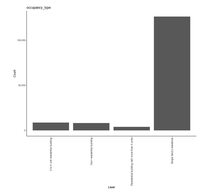
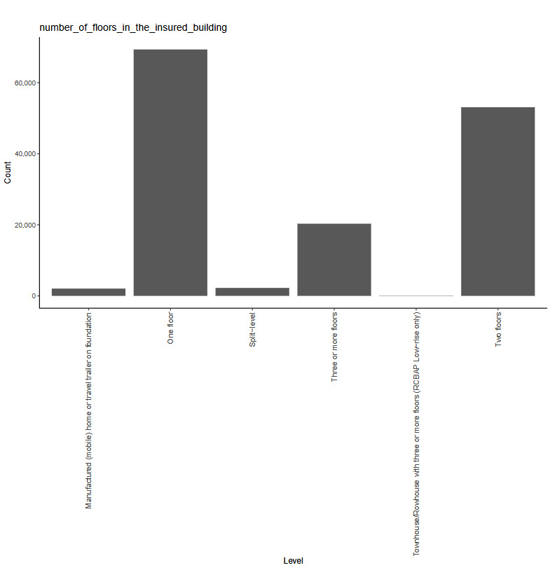
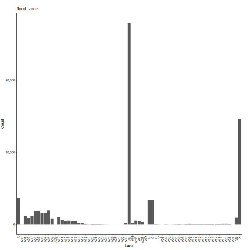
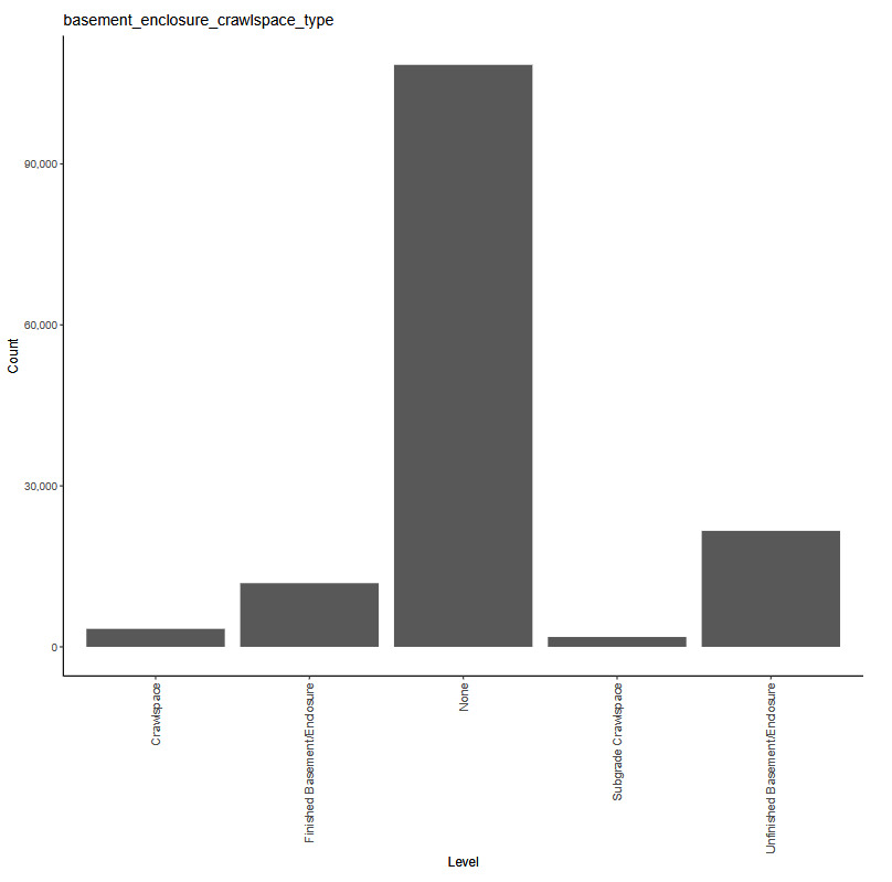
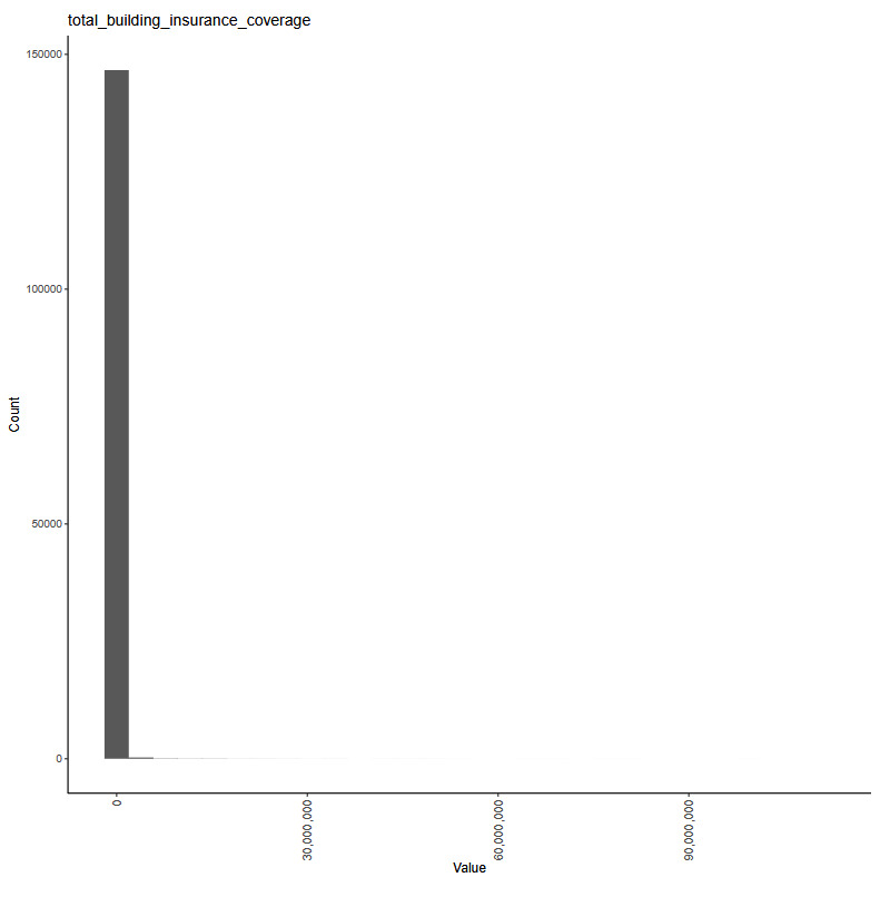
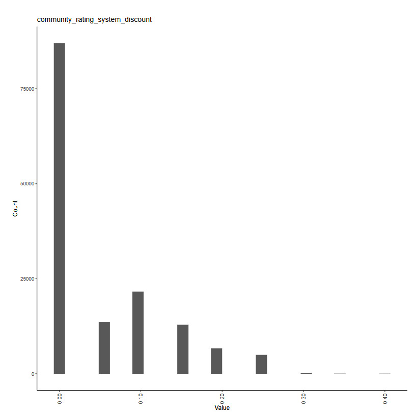
The working example for our experiments is as follows: Given a set of claim characteristics, we predict the losses paid on the property coverage of the policy. The data we use comes from the NFIP and is made available by the OpenFEMA initiative of the Federal Emergency Management Agency (FEMA).^[1] Two datasets are made available by OpenFEMA: a policies dataset with exposure information and a claims dataset with claims transactions, including paid amounts. Because there is no way to associate records of the two datasets, we are limited to fitting severity models on the claims dataset. While the complete dataset contains more than 2 million transactions, for the purposes of our experiments, we limit ourselves to data from 2000 to 2019 and further subsample 100,000 data points to make experiments feasible on a CPU. The dataset includes a rich variety of variables, from occupancy type to flood zone, and a brief exploratory data analysis can be found in Appendix 7. For our models, we work with a few selected variables that represent continuous and discrete variables of low and high cardinalities, which we list in Table 4.

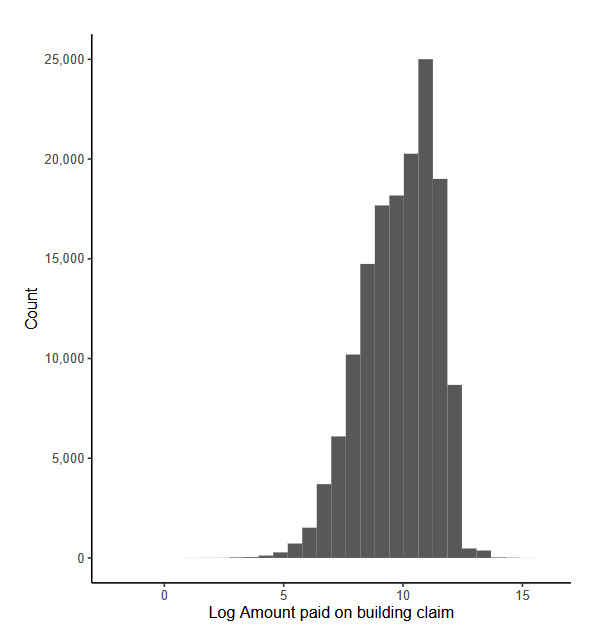
The response variable we take from the dataset is “Amount paid on building claim,” which is a numeric variable.

For our experiments, we set up a fivefold cross-validation scheme and apply it to each of the models we introduce. In Sections 4.2 and 4.3, the tables and figures are based on a single fold of the cross-validation split. In Section 4.4, we provide the cross-validated performance metrics of each of the models.

Whereas the main focus of our contribution is on applications of categorical embeddings in predictive modeling, we have fine-tuned the neural network models in this (and the next) sections using the same fivefold cross-validation scheme described above, but applied to a separate 100,000 data point subsample of the NFIP data. The results of this fine-tuning are reported in detail in the appendix, and this separate subsample of the NFIP data is not used for any other purpose in this study. The performance metrics in this, and the next, section are based on the optimal models found through this process. Our aim is to show that one can quite easily develop performant predictive models using categorical embeddings and that one can enhance those models using suitable architectures utilizing attention mechanisms. As we describe the modeling procedure and results, we provide further commentary on recommended practices in practical applications, especially with respect to the neural network models.

4.2. Models

In this subsection, we develop the following models:

1. A GLM with gamma distribution and log-link function

2. A neural network with one-dimensional categorical embeddings

3. A GLM with the categorical predictors replaced by the learned embeddings from Model 2

4. A neural network with multidimensional categorical embeddings

These model architectures are relatively uncomplicated by today’s standards, and they are so chosen to better highlight the embedding components. Later, in Section 5, we investigate more involved architectures using embeddings that represent the state of the art for modeling tabular data.

4.2.1. Model 1: GLM

While this paper focuses on embeddings in neural networks, we begin with a GLM to provide a common frame of reference, since most actuaries are familiar with the technique. Although GLMs are commonplace and well studied in the actuarial literature, there are still plenty of decisions to be made in the modeling process—see, for example, Goldburd et al. (2020) for an in-depth discussion. For our purpose of establishing a baseline, we proceed with what we perceive as reasonable decisions with regard to feature engineering and model structure, outlined thus:

• Target variable: Amount paid on building claim

• Predictors:

  • \(\log\) building_insurance_coverage

  • basement_enclosure_type,

  • number_of_floors_in_the_insured_building

  • prefix of flood_zone

  • primary_residence

• Link function: \(\log\)

• Distribution: gamma

We take the log of the continuous predictor building_insurance_coverage, which allows the scale of the predictor to match that of the target variable. Because the flood_zone variable in the original data contains 60 levels, we take the prefix of the zone code, which corresponds to the level of risk as determined by FEMA.^[2] For example, "A01", "A02", and so on are recoded as simply "A". A log link together with the gamma distribution is a standard choice for severity modeling, which provides a multiplicative structure where the response is positive. Following the notation in 3.1, the number of parameters in the GLM is

\[1 + |J^{\text{num}}| + \left(\sum_{j \in J^{\text{cat}}} n_{\mathcal{P}}^j\right) - |J^{\text{cat}}|: \tag{9}\]

one for the intercept, one for each numeric variable, and the numbers of levels minus one (due to dummy coding) for each categorical variable.

In Table 5, we exhibit an excerpt of the relativities, or exponentiated fitted coefficients, of a couple of the categorical variables. Recall that the choice of the log link gives a multiplicative structure, so the interpretation of 1.35 for occupancy_type = "Non-residential building" is that, all else equal, the expected loss for a policy for a nonresidential building is 1.35 times that of a policy for a single-family home, which is the base, or reference, level for the factor.

4.2.2. Model 2: Neural network with unidimensional embeddings

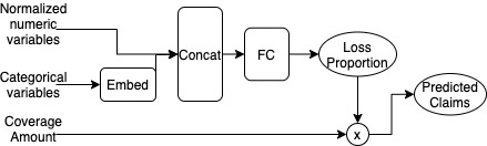
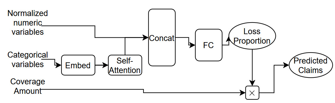
For Model 2, we build a feedforward neural network whose architecture is shown in Figure 1. The categorical inputs go through one-dimensional embedding layers where they are each mapped to a scalar. The embeddings are then concatenated with the numeric predictors, which have been normalized in data preprocessing, before being passed through a feedforward layer (with eight hidden units and ReLU activation) to finally obtain a scalar value between 0 and 1, as constrained by a sigmoid output activation. Some regularization is applied within this network using the dropout technique of Srivastava et al. (2014) with a dropout rate of 2.5% and by early-stopping the fitting of the network by selecting the model weights that relate to the lowest estimated mean squared error (MSE) score on a 5% validation sample. Dropout functions by setting some components of the network randomly to 0 during each epoch of training. This forces each component of the network to learn a somewhat independent representation of the data, thus helping to avoid overfitting by preventing components of the network from becoming too specialized. This scalar output represents the proportion of coverage amount that is paid out, which we then multiply by the dollar amount of the coverage amount to obtain our prediction of the claims paid. For optimization, we use the MSE loss function.

With a single hidden layer, this architecture is relatively simple; without the hidden layer and corresponding ReLU activation, we would actually recover a type of logistic regression structure. The choice of one for the embedding dimension is also due to simplicity: It is easily interpretable as the representation of each factor level as a point on the real number line; also, the trained embeddings are easily incorporated into a GLM, which we will see in Model 3. In practice, the embedding dimension is a hyperparameter one can tune, for example via cross-validation, and can vary for each variable. However, we also note that the choice of one for the embedding output dimension is not an unreasonable one, especially when the cardinalities of the categorical variables are not large (i.e., when they are in the 10s).

In Tables 6 and 7, we show the learned embeddings for occupancy_type and an excerpt of them for flood_zone. While it may be tempting to compare these values to those in Table 5, they represent fundamentally different concepts. It is helpful to think of the embedding values for each variable as a continuous representation of the variable itself, rather than a “coefficient” associated with the variable. Note that it is not straightforward to inspect the embeddings from a table and infer relationships to the response variable, even in a shallow network such as ours, due to nonlinearities within the model. Also note that we now have a way to incorporate the full granularity of the flood_zone variable, which is why more levels are shown in Table 7 than in Table 5. In Section 4.3, we discuss techniques to visualize these embeddings.

4.2.3. Model 3: GLM with neural network embeddings

For Model 3, we return to the GLM, but now we replace the categorical variables with the trained embeddings from Model 2. In other words, our model now contains only continuous variables, and each categorical factor is represented as a scalar value and obtains its own coefficient. In contrast with the number of parameters computed in Equation (9), we have fewer parameters for this model:

\[1 + |J^{\text{num}}| + |J^{\text{cat}}|. \tag{10}\] Hence, the model can be written as

\[\mu_i = \beta_0 + \sum_{j \in J^{\text{num}}}\beta_{j} x_{i,j} + \sum_{j \in J^{\text{cat}}} \beta_{j} z_{i,j},\tag{11}\]

where \(z_{i,j}\) represents the embedding value for the \(i\)th instance of the categorical column \(X_j\).

Although, in this particular example, we incorporate one-dimensional embeddings, one can easily include multidimensional embeddings, which would increase the model’s flexibility. The modeler would need to balance the potential additional lift with overfitting and some loss of interpretability, since, with one-dimensional embeddings, our GLM structure dictates that there is a monotonic relationship between the predicted response and the input embedding, which could be desirable in certain use cases (and undesirable in others).

Regardless of the hyperparameters chosen, care needs to be taken in ensuring the integrity of the model validation process, since when we train the embeddings, we utilize the information from the response variables. Therefore, the holdout data must not be seen by the neural network training process or the GLM fitting process.

Since we only have a few parameters in this model, we exhibit the full list of fitted coefficients in Table 8. For each categorical variable, there is only one coefficient estimate. This is because each categorical variable has been replaced by a single scalar value, so we treat it as if it were any other continuous predictor.

An interesting ramification of our choice of embedding dimension of 1 in this example is that we can compute the “implied relativities” of the factor levels in the new GLM. Since each level corresponds to a unique scalar value, we can obtain its contribution to the linear predictor by multiplying by the coefficient estimate of the variable. For example, multiplying the estimate of 2 for occupancy_type in Table 8 by each value in Table 7, we obtain the unnormalized contributions of each level, which can then be exponentiated and normalized with respect to the base level Single-family residence in order to obtain the implied relativities, which could then be compared with the first GLM’s output in Table 5.

4.2.4. Model 4: Neural network with multidimensional embeddings

Model 4 is architecturally identical to Model 2, with the only difference being the number of embedding dimensions. Instead of mapping factor levels to real numbers, we map them to points in Euclidean space, where the dimension of the space is the ceiling of the factor’s cardinality divided by 2. Formally, in the notation of Section 3.1, \(q_{\mathcal{P}^j}=\lceil{n^j_{\mathcal{P}}/2}\rceil\) for variable \(X_j\). Following the discussion thus far, we list the learned embeddings for a couple of variables in Tables 9 and 10. Note that for flood_zone, we are displaying the embedding for only one level.

4.3. Visualization techniques for interpretation

With artificial intelligence and machine learning coming into the mainstream across industries and use cases, the topic of model explainability has received increasing attention. In insurance pricing, Kuo and Lupton (2020) propose a framework for model interpretability in the context of regulation and actuarial standards of practice, while Henckaerts et al. (2020) investigate algorithm-specific techniques to inspect tree-based models. Kuo and Lupton (2020) and references therein also discuss commonly used model-agnostic explanation techniques, such as permutation variable importance and partial dependence plots, that can be applied to the neural networks we consider in this paper.

In this section, we focus on ways to visualize the learned embeddings. In the authors’ experiences, oftentimes the formats of the visualizations—basic line and scatterplots—even more so than the content of the data, are helpful in explaining the concept to stakeholders.

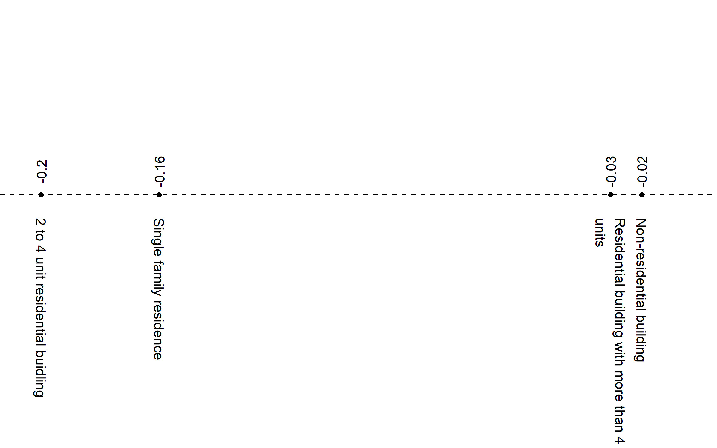
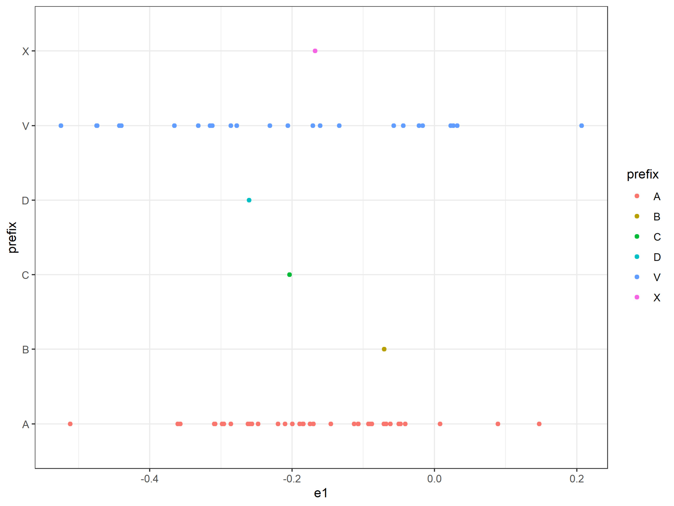
For Model 2, the neural network with one-dimensional embeddings, the task is simple: We can plot the levels on a line, as in Figure 2. In the case of flood_zone, where we happen to have the luxury of knowing a priori the meaning of the prefixes, we can plot them separately, as in Figure 3, to see how the model mapped them.

For Model 4, the neural network with multidimensional embeddings, we would need to treat the learned values before we can plot them. Specifically, we need to reduce the dimension of the data to 2D for embeddings with more than two dimensions. The standard approaches for this are principal component analysis (PCA; Shlens (2014)) and t-distributed stochastic neighbor embedding (t-SNE; Maaten and Hinton (2008)), both of which we illustrate. For a technical review of these methods, refer to Appendix 9.

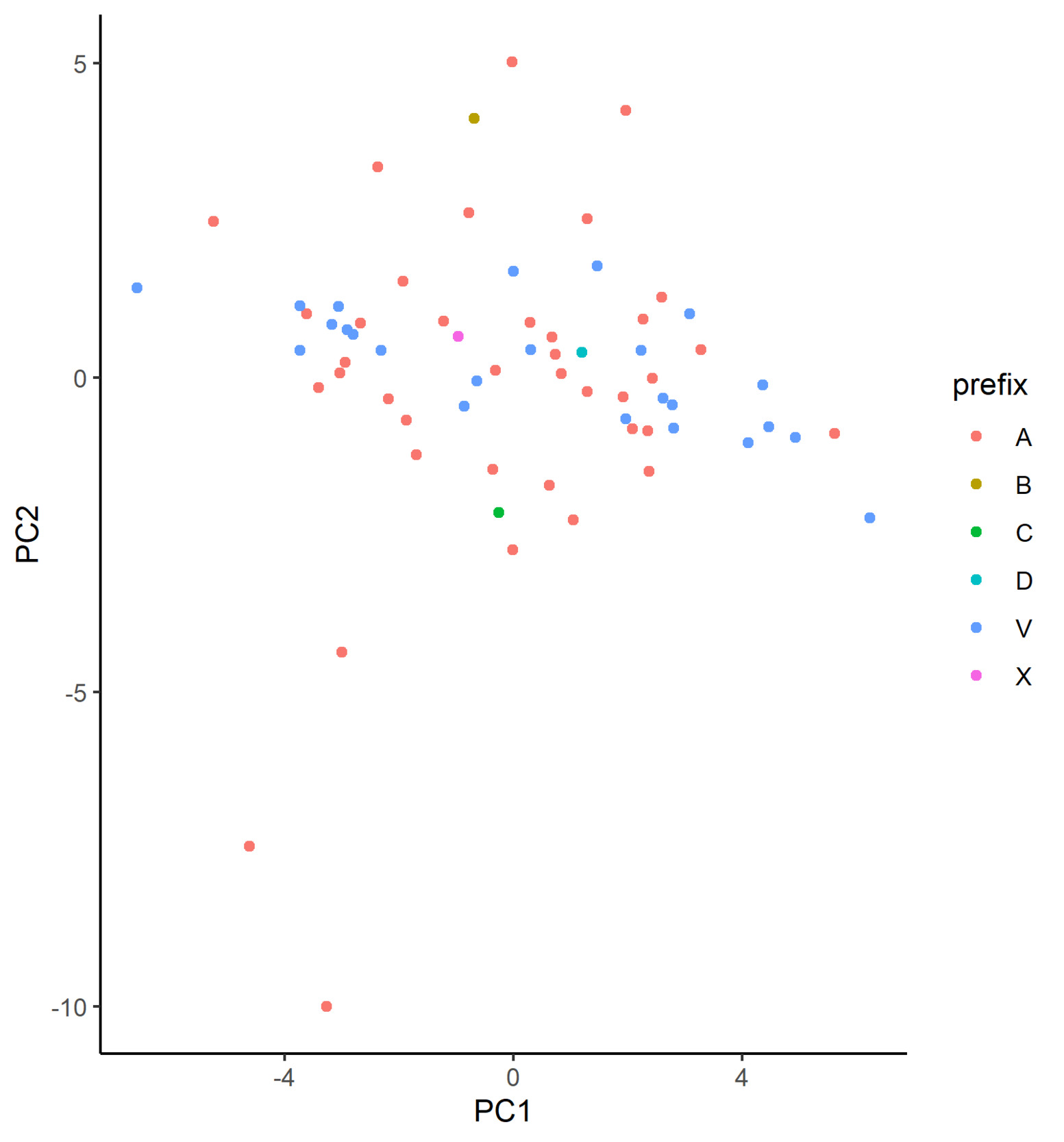
In Figure 4, we plot the learned embeddings for flood_zone in Model 3 on the coordinate system defined by the first two principle components. In our case, however, we are not able to identify discernible clusters in the plot. From inspecting the matrix decomposition results, we see that the cumulative proportion of variance for the first two principal components is just 0.38, which is a relatively low proportion, suggesting that perhaps PCA is not the most appropriate dimensionality reduction technique in this case. Additionally, this indicates that each of the dimensions of the calibrated embeddings is important, implying that the embedding has been well calibrated.

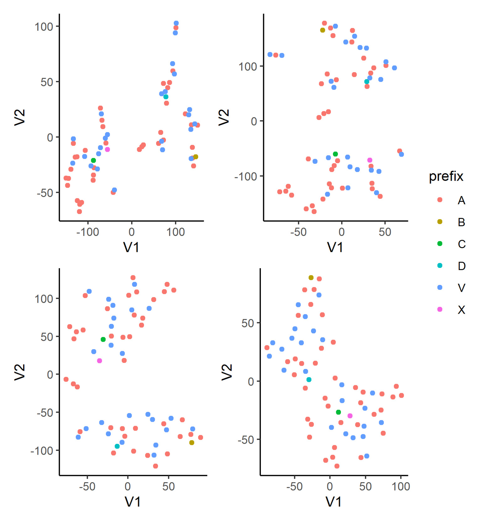
In Figure 5, we display the t-SNE of the learned embeddings for flood_zone in Model 3 with various perplexity settings: 2, 3, 5, and 10; the learning rate and the number of steps are fixed at 100 and 10,000, respectively, for all plots. In the first three plots, we can see the semblance of clusters forming. In particular, flood zone B appears at the extreme of the plot, which implies it is relatively far away from other levels in the embedding space, as seen by the model. We also observe that flood zones C and X lie close to each other, regardless of the perplexity parameter, and a similar observation can be made for flood zones B and D. Using those two sets of points as anchors within these plots, we can finally observe that the learned embeddings for flood zones A and V appear to be divided into two main groups. While t-SNE is a powerful visualization technique, there are a few points the modeler should be mindful of in practice. We refer the reader to Wattenberg et al. (2016) for a more thorough discussion but stress here that the resulting plot can be very sensitive to the perplexity hyperparameter. In addition, for our use case, which is to explore the learned embeddings, we have fewer data points than most other applications in the literature. Accordingly, our reasonable range of hyperparameter values is adjusted down.

4.4. Training and inference

For the GLMs, Models 1 and 3, we follow the standard optimization procedure using iteratively reweighted least squares without regularization. For the neural networks, Models 2 and 4, we utilize the Adam optimizer (Kingma and Ba 2014) with a learning rate of 0.001 and a minibatch size of 1,024. Using a fivefold cross-validation approach, we split the dateset into analysis and assessment sets, containing 80% and 20% of the rows, respectively, and further select a 5% sample of the analysis set as a validation set to estimate the out-of-sample performance of each model. This is repeated five times on non-overlapping subsets of the dataset. For each of the five splits of the data, we train on the analysis set for a maximum of 150 epochs and select the best model from the 150 epochs as measured by the validation set. Finally, as mentioned above, in addition to this form of early stopping, we also apply the dropout technique with a rate of dropout of 2.5%.

During inference, or scoring, care must be taken to accommodate the categorical levels that are unseen during training. While we allow for an extra key in the embedding dictionary, the initial weights are not updated during training, which could lead to nonsensical predictions in the validation or test sets. To circumvent this issue, before applying the trained model but after the final optimization epoch, we update the weights for the unseen levels manually. In practice, a common approach is to take an average value of some sort of the weights of the other levels. In our case, we take the median (if there are multiple, the lower of the two), but a mean, a mean weighted by frequency of observations, or a trimmed mean could be used.

In Table 11, we exhibit the cross-validated performance metrics of each of the models. We report both the root mean squared error (RMSE) and the mean absolute error (MAE); we note that these are just two of many potential metrics we could use, and they are so chosen for their interpretability and prevalence in the literature for comparing different types of models. Recall that, between the two metrics, RMSE penalizes large mispredictions than MAE. Also, in the optimization process, a GLM with a gamma distribution optimizes the deviance, rather than MSE directly.

We see that the neural networks outperform the GLMs in all cases, as would be expected. What is more interesting is that using learned embeddings in place of categorical levels improves the GLM, at least from the RMSE perspective. This indicates that using neural networks to derive embeddings for categorical variables for subsequent use in GLMs is a strategy that modelers should consider when building GLM models for ratemaking.

While linear regression (i.e., the specific case of a GLM with a Gaussian distribution and identity link function) is not commonly used for severity modeling, we add it into the mix as a benchmark, a practice we recommend in order to check the reasonableness of other models’ results. Because it is possible for a linear regression to output negative values, we cap the predictions below by 0.01 during scoring. Somewhat surprisingly, in the problem we are considering, the linear model performs slightly worse than the more complex neural network models in the RMSE metric but significantly better than the other GLM models. This may be because this model optimizes for the RMSE metric, as the unit deviance of the normal distribution corresponds to MSE. Conversely, the linear model’s performance is quite significantly worse on the MAE metric. Another observation is that Model 4 performs slightly worse than Model 2, perhaps as a result of some overfitting resulting from the multidimensional embeddings in Model 4. If further tuning were to be applied, it would be sensible to apply extra regularization to Model 4; however, we refrain from doing so here.

5. Attention-based modeling

In this section, we investigate whether we can improve the predictive performance of the models applied to the NFIP dataset by applying the attention-based models defined in Section 3.2.2. We discuss the implementation of each of the simple attention, TabTransformer, and TabNet models in the following subsection. We then discuss how the modifications made to the embeddings through the application of attention can be visualized in the following subsection. We conclude with a discussion of the model results.

5.1. Models

In this subsection, we develop the following models:

1. A neural network based on the design of Model 4, with an attention component

2. Similar to Model 5, a neural network implementing the TabTransformer architecture

3. A neural network implementing the TabNet architecture

Compared with the models presented in the previous section, the models presented here are closer to state-of-the-art models that might be used for tabular data modeling problems. To the best of our knowledge, this is the first analysis of these architectures in the actuarial literature.

5.1.1. Model 5: Simple attention network

Model 5 is conceptually similar to Model 4, except for the following two aspects. First, we standardize the dimension of the embedding layers to eight dimensions for each categorical covariate. This is done to allow for the application of the attention component, which requires the embeddings for each covariate to have the same dimension. Second, we apply a self-attention mechanism within the network, as shown in Equation (8). We illustrate this architecture in Figure 6.

5.1.2. Model 6: TabTransformer

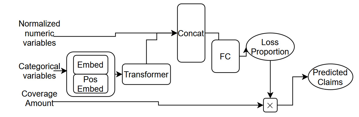
Whereas Model 5 makes a simple modification to the structure of Model 4, the TabTransformer model is slightly more complex. With respect to similarities between Models 5 and 6, both use embeddings with a standard eight dimensions for each categorical covariate. In terms of differences, Model 6 uses a transformer layer in place of self-attention and a positional encoding of a single dimension, i.e., \(d_{col} = 1\). The TabTransformer architecture is shown in Figure 7.

5.1.3. Model 7: TabNet

The final model we consider in this subsection is the TabNet architecture. In TabNet, similar to decision trees, by which it is inspired, the input features are processed sequentially in a number of decision steps. In each decision step, a different subset of features are weighted more than the rest based on masks defined by attention modules applied to information from the previous step. The output of each step consists of information for the next decision step and also an output representation that is set aside and then aggregated at the end, along with other decision step outputs, in order to produce the final model output. Due to the complexity, we refer the reader to Arık and Pfister (2019) for the full architectural details.

5.2. Training and inference

We follow a training setup for the three attention-based models similar to that used for the neural networks discussed in the previous section. For Models 5 and 6, we use the Adam optimizer as before, and similar to the models in the previous section, we use a learning rate of 0.001. Similarly, we train on the analysis set for a maximum of 150 epochs and select the best model based on the lowest loss achieved on the assessment. Moreover, because these models are significantly more complex than those tested in the previous section, we also add extra regularization using dropout to the attention layers, to prevent overfitting. In this section, we drop out components with a probability of 2.5%. A final detail is that, for both of these models, we use an embedding dimension of size 16 for each of the categorical covariates, since the attention mechanism requires that the embeddings be of a common length. For the TabTransformer model, we use a row embedding of dimension 4.

For Model 7, we use the suggested training setup that utilizes the Adam optimizer with a learning rate of 0.02 and train for 15 epochs (since longer training times did not lead to improved performance).

In Table 12, we show the cross-validated performance metrics of each of the models, as well as the two best-performing models from the previous section. As before, we report both the RMSE and the MAE. The results show that Model 5, which simply adds attention to Model 4, outperforms Model 4 on both the RMSE and MAE metrics. Thus, there is some room to argue that for tabular data modeling that uses embeddings for categorical data, the use of attention within models should be considered. The TabNet architecture performs poorly, perhaps due to insufficient hyperparameter tuning, but indicating that out of the box, TabNet does not appear to work well for this modeling task. Finally, the TabTransformer model shows the best performance of all models considered in this research, beating the other models by a significant margin on both the RMSE and MAE metrics. We conclude that the more complex transformer-style attention applied in the TabTransformer model appears to lead to a relatively significant improvement in performance over all other models considered here.

In what follows, we focus on understanding the TabTransformer model in more detail.

5.3. Exploring the TabTransformer model

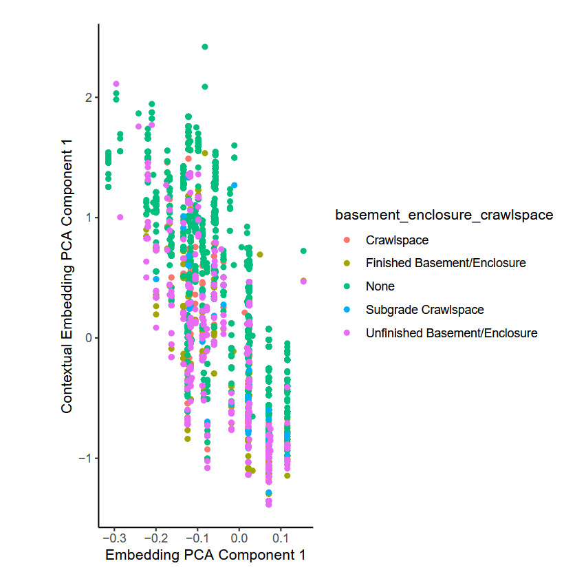
Here, we explore what the TabTransformer model has learned from the data via the attention process that forms the core of the model. We focus on the difference between the flood embedding learned by the model, compared with the output of the transformer layer that processes the embeddings before they enter the model. Huang et al. (2020) call the latter contextual embeddings because the attention mechanism in the TabTransformer model augments the embeddings based on the other covariates that appear for each observation \(i\).

To illustrate this, we selected a single TabTransformer fit on one fold of the training data and selected at random 10,000 individual observations. For each observation, the embedding relating to the flood zone of the observation was extracted from the model, as well as the contextual embedding that was produced for that observation by the TabTransformer model. We found that a PCA and t-SNE analysis of the embeddings produced very similar results to those shown in the previous section, so we do not show those plots here. To investigate the difference between the embeddings and contextual embeddings for the flood_zone variable, we show the first component from a PCA analysis of each of these in Figure 8.

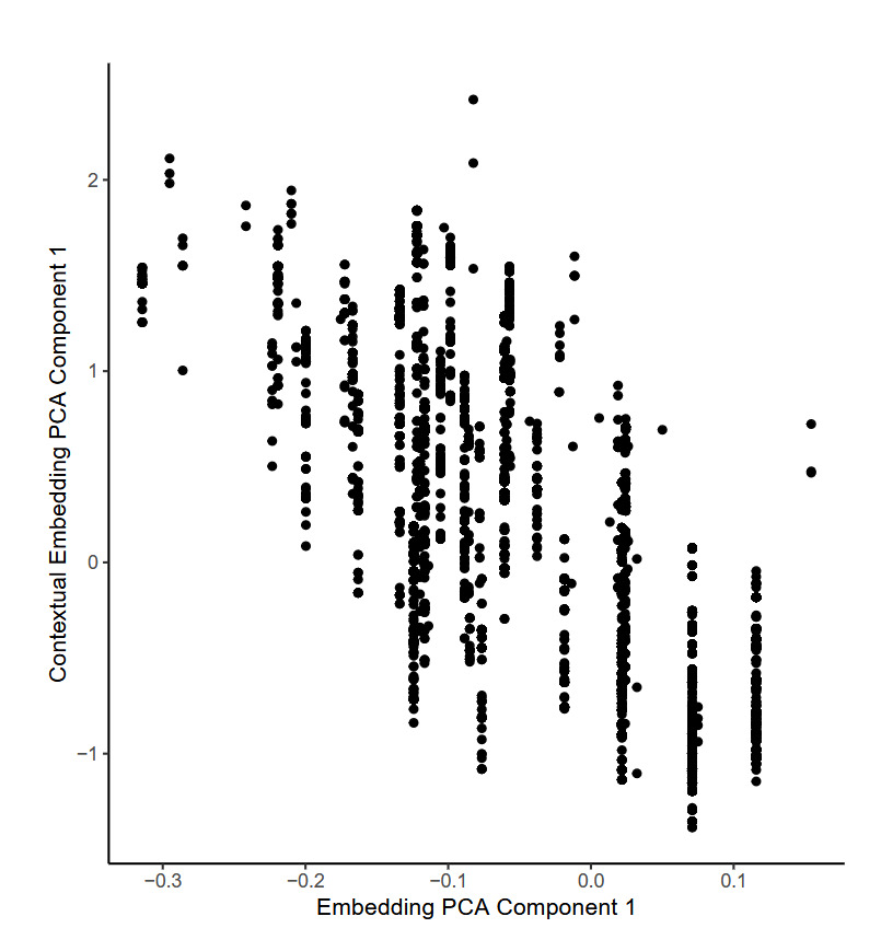
The figure shows that whereas the first principal component of the embeddings occupies discrete points only (shown on the \(x\)-axis), the first principal component of the contextual embeddings is continuous (shown on the \(y\)-axis), meaning that the model has modified the values of the embedding in a smooth manner. Since the inputs to the attention mechanism that is responsible for this are the embeddings for the other categorical variables for each observation, those other variables have influenced the final embedding used within the model for the flood_zone variable. By considering each of the other categorical variables entering the model, it was found that the basement enclosure crawl space variable explains most of the variation observed within the flood zone embeddings, as Figure 9 shows. The attention mechanism produces the lowest values for those observations with an unfinished basement, whereas the model produces the highest values for buildings without a crawl space.

To investigate the predictive value added by the contextual embeddings, we fit a simple gamma GLM to these 10,000 observations, with the goal of predicting the claim amount based only on either the embeddings or the contextual embeddings. As Table 13 shows, the performance of the latter model, as indicated by the RMSE and MAE metrics, is better—in other words, the contextual embeddings that incorporate information across all of the categorical variables are better predictors of claim severity compared with the embeddings.

6. Conclusions

This study focuses on how embeddings can be applied in the context of actuarial modeling by illustrating a range of approaches. First, we define relatively simple neural networks. We reuse the embeddings from those models in traditional GLM models. Lastly, we study more advanced attention-based models. These models were demonstrated within the context of a claims severity modeling problem based on data from the NFIP. Whereas we consider only severity in this study, it is likely that our findings will replicate for the modeling of claim frequency, which is usually an easier problem. Our key findings are that processing categorical variables with multidimensional embeddings leads to enhanced performance within simple neural networks and that including these within traditional GLM models can enhance those models’ predictive performance, compared with the usual encoding scheme for categorical variables. Some of the attention-based models we looked at performed well; in particular, the TabTransformer model of Huang et al. (2020) appears quite promising for use in actuarial modeling. The study also illustrates how embeddings can be visualized using the PCA and t-SNE techniques. We find that in the case of the NFIP data, it is possible to explain which variables modify the embeddings based on the context of each observation.

We posit several avenues for future research. One surprising finding is that the TabNet model performed quite poorly, leading us to conclude that it is not particularly suitable for actuarial modeling. Understanding that finding in more detail would be a valuable contribution to the literature. Another helpful contribution would be to investigate the optimal hyperparameters for the TabTransformer model in the context of actuarial modeling. Lastly, extending our findings to a claims frequency example could be considered.

---

Acknowledgments

We thank the two anonymous reviewers for their helpful comments, which significantly improved the manuscript.