Graph-Based Embedding for Categorical Features in Actuarial Applications

1. Introduction

Categorical variables play a crucial role in non-life actuarial applications, particularly in risk classification and predictive modeling. First, many variables widely used in insurance domains are qualitative, such as vehicle model and make in automobile insurance or construction and roof type in property insurance. Second, categorical variables are also key to creating risk classes, which are integral to pricing and underwriting processes. Third, in practice, actuaries often discretize continuous numeric variables into categories to account for potential nonlinear effects of rating variables.

The focus of our research lies in the treatment of categorical variables with latent patterns and structures—an area of significant complexity but one that has received less attention in the literature. While categorical variables are typically used to denote group labels or classifications, in many actuarial contexts, they exhibit intricate structures. Examples include postal codes, which capture geographical proximity and spatial relationships, vehicle models and makes, which involve hierarchical associations, and fire rating classes, which naturally embody a form of ordering. These inherent patterns and structures often remain unexploited in traditional methods of modeling categorical variables. In this paper, we introduce a knowledge-driven embedding method, formulated as an unsupervised learning approach, to derive numerical representations of categorical variables. The aim is to capture not only the individual characteristics of each categorical level but also the nuanced relationships and latent structures embedded within such variables. This approach stands in contrast to conventional methods, which may overlook such complexities, leading to suboptimal representations in predictive models.

The most widely used technique for handling categorical features in predictive models is one-hot encoding. That method converts a categorical variable into a set of binary indicators, each representing a unique category. For instance, a categorical variable with three levels is represented by \((1,0,0)\), \((0,1,0)\), and \((0,0,1)\). While one-hot encoding is suitable when the number of categories is small, it becomes problematic when applied to variables with a large number of levels, a common occurrence in actuarial applications. High cardinality can lead to several issues: First, it results in high-dimensional input data, increasing computational demands; second, it may cause small sample sizes for certain categories, leading to greater uncertainty in parameter estimates; and third, one-hot encoding fails to capture the inherent relationships between categories, such as latent subgroups or hierarchies. To address these limitations, alternative methods have been proposed in the literature. Notable contributions include Antonio and Beirlant (2007), Guiahi (2017), Richman (2021), Blier-Wong et al. (2022), and Avanzi et al. (2024), among others. One particularly promising approach is categorical embedding, a neural network–based method that seeks numerical representations for categorical variables. The approach generates low-dimensional embeddings where categories that are closer in distance exhibit similar behavior, thus improving the ability to model latent relationships (see Shi and Shi (2023); Delong and Kozak (2023); Shi and Shi (2024)).

Building on that body of work, our research focuses on high-cardinality categorical variables with complex latent structures. While existing methods have proven effective in traditional scenarios, they often fail to fully exploit the wealth of information contained within categorical variables, leading to information loss and suboptimal model performance. For instance, geographical data such as counties or census tracts involve spatial relationships, and variables such as vehicle models or medical diagnosis codes contain hierarchical associations. Such structures are not adequately captured by existing embedding techniques, which is where our proposed method aims to make a significant contribution.

Our approach addresses these shortcomings by constructing numerical representations that preserve the latent patterns and structures of categorical variables. The method, which is inherently unsupervised, consists of two key steps: First, we construct a graph to represent the complex relationships and domain-specific insights associated with the categorical variables; second, we apply state-of-the-art graph neural embedding techniques to transform the graph structures into meaningful numerical representations. As a result, our method generates embeddings that not only capture generic information but also encapsulate the distinct nuances, correlations, and hierarchies inherent in each categorical variable. This leads to substantial improvements in the numerical representation of categorical variables in insurance analytics. Compared to existing embedding methods, our approach offers several advantages. First, we offer a fresh perspective on representing categorical variables, focusing on preserving the intrinsic information within complex structures. This enhances the accuracy and relevance of the variables when used in predictive models. Second, whereas many embedding methods rely on complex machine learning models such as deep neural networks, our approach is more interpretable. It does not require an output variable, allowing it to easily incorporate domain knowledge and making it applicable in a broader range of downstream tasks.

In the empirical analysis, we showcase the effectiveness of our proposed method using a real-world dataset from the automobile insurance industry. Our focus is on the categorical variable “geographical region,” which serves as a critical factor in risk assessment and pricing in non-life insurance applications. We explore two distinct scenarios to highlight the versatility and practical value of our approach. In the first, we address risk classification, showing how our method captures latent relationships between regions, generating risk clusters that enhance premium pricing and risk management. In the second, we focus on pricing new risks, demonstrating that our method produces reliable estimates based on the spatial structure of the data, offering a robust solution for pricing risks in new territories.

Our research makes several important contributions to the literature. First, the widespread use of categorical variables in actuarial practice highlights the practical relevance of our method. By generating precise numerical representations of these features, insurers can improve decision-making processes and maintain a competitive advantage in the ever-evolving insurance landscape. Second, this study serves as a pioneering project, laying the groundwork for feature construction methods applicable to nontraditional data that extend beyond categorical variables. This expands the potential applications of our method across a broader range of insurance analytics. Third, we contribute to the wider body of predictive modeling literature in actuarial science. Predictive modeling has become a cornerstone of modern actuarial practices, particularly in areas such as ratemaking, claims reserving, and claims management (see Frees et al. (2014) and Blier-Wong et al. (2021)). Insurers constantly seek ways to integrate more comprehensive information into their models to gain a competitive edge. One of the major challenges in this process is minimizing information loss during feature construction, as the complex details inherent in the original data may not always be fully captured in modern statistical and machine learning models. This issue has become even more pressing in the big data era, where data complexity and diversity continue to grow. Our work addresses this challenge by providing a method for embedding categorical variables with latent and complex structures, preserving the richness of the original data.

The rest of this paper is organized as follows: Section 2 presents the knowledge-based embedding method. Section 3 provides the data analysis and case studies. Section 4 concludes the paper.

2. Method

This section outlines the methodology employed to effectively handle high-cardinality categorical variables with latent patterns and structures in actuarial applications. We introduce a knowledge-driven embedding approach that leverages graph-based representations and graph neural embedding techniques to capture intricate relationships within categorical data. The methodology is divided into two primary components: graph construction and graph node embedding.

2.1. Graph construction

Graphs are a versatile and powerful data structure for representing complex systems, capable of capturing intricate relationships through nodes and edges. In this framework, nodes represent objects or entities, while edges signify interactions, connections, or dependencies between those entities. Formally, a graph \(G(V;E)\) consists of a set of vertices denoted by \(V = \left\{ v_{1},\ldots,v_{n} \right\}\) and a set of edges denoted by \(E = \left\{ e_{ij} \right\}_{i,j = 1}^{n}\), where each edge \(e_{ij}\) connects a pair of vertices \(v_{i}\) and \(v_{j}\).

One commonly used mathematical representation of a graph is the adjacency matrix, denoted by \(A \in \mathbb{R}^{|V| \times |V|}\), which captures the connections between nodes. In this matrix, an element \(a_{ij}( \geq 0)\) indicates the weight or strength of the edge \(e_{ij}\), representing the intensity or significance of the relationship between nodes \(v_{i}\) and \(v_{j}\). For undirected graphs, the adjacency matrix \(A\) is symmetric, reflecting that connections are bidirectional. In contrast, directed graphs may have asymmetrical adjacency matrices to represent directional relationships. This structure is widely applicable across various domains, such as social networks, biological systems, transportation networks, and communication systems, providing a rigorous mathematical framework to analyze and model both individual entities and the connections linking them.

In the context of our study, the goal is to construct a graph to represent categorical variables, facilitating the creation of numerical representations for different categorical levels. Categorical variables are types of variables that represent data in distinct categories or groups, are often used to categorize or label data points, and are particularly useful for representing qualitative or descriptive information. While generic categorical variables (e.g., blood type, education level) may lack explicit intercategory relationships, those with latent structures—such as geographical regions, vehicle models, or hierarchical classifications—can benefit significantly from graph representations. This approach allows us to capture spatial proximity, hierarchical dependencies, and other complex intercategory relationships that traditional encoding methods often miss, making these structured categorical variables the focus of our study.

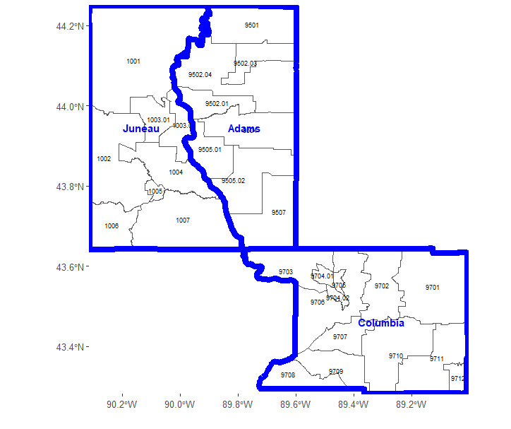
Graphs, as abstract data structures, provide a versatile framework for representing complex relationships and offer considerable flexibility in their construction. The specific way in which a graph is built depends on the problem context and the relationships among the categories being modeled. For a categorical variable with \(L\) levels, each level can be represented by a node, denoted \(v_{i}\) for \(i = 1,\ldots,L\). However, the construction of edges between these nodes is not fixed and can vary depending on how the categories are interrelated. The edges, which connect the nodes, reflect the relationships between the categories, and their construction is shaped by the underlying data structure and dependencies. Here, we outline guidelines and methods for building graphs, illustrated through practical examples. We use geographical region variables—census tracts and county names within Wisconsin—to demonstrate the construction of a graph that captures the inherent relationships among categorical levels. Census tracts and counties are statistical geographical entities, where a county serves as a larger administrative division within a state, and census tracts represent smaller, more granular statistical subdivisions within each county. Figure 1 shows three counties in Wisconsin—Juneau, Adams, and Columbia—and their corresponding census tracts, each labeled with a unique identifier. These counties contain a total of 29 census tracts, with eight in Juneau, eight in Adams, and 13 in Columbia. Thus, the census tract variable comprises 29 distinct levels, and our goal is to construct a graph to represent these census tracts and the relationships between them, enabling a structured numerical encoding for subsequent analysis. In the following, we present two alternative approaches to construct graph edges: one based on geographical adjacency and the other based on geographical proximity.

Figure 1.Map of Juneau, Adams, and Columbia counties in Wisconsin.

2.1.1. Geographical adjacency

This method establishes connections between nodes (census tracts) that are geographically adjacent. Formally, the edge set is defined as

\(E = \left\{ e_{ij} = \left( v_{i},\ v_{j} \right)\ |\ v_{j}\mathcal{\in \ A}\left( v_{i} \right) \right\}\),

where \(\mathcal{A}\left( v_{i} \right)\) represents a set of nodes adjacent to \(v_{i}\), i.e.,

\(\mathcal{A}\left( v_{i} \right) = \left\{ v_{j} \in V\ |\ v_{i}\ and\ v_{j}\ are\ geographically\ adjacent \right\}\).

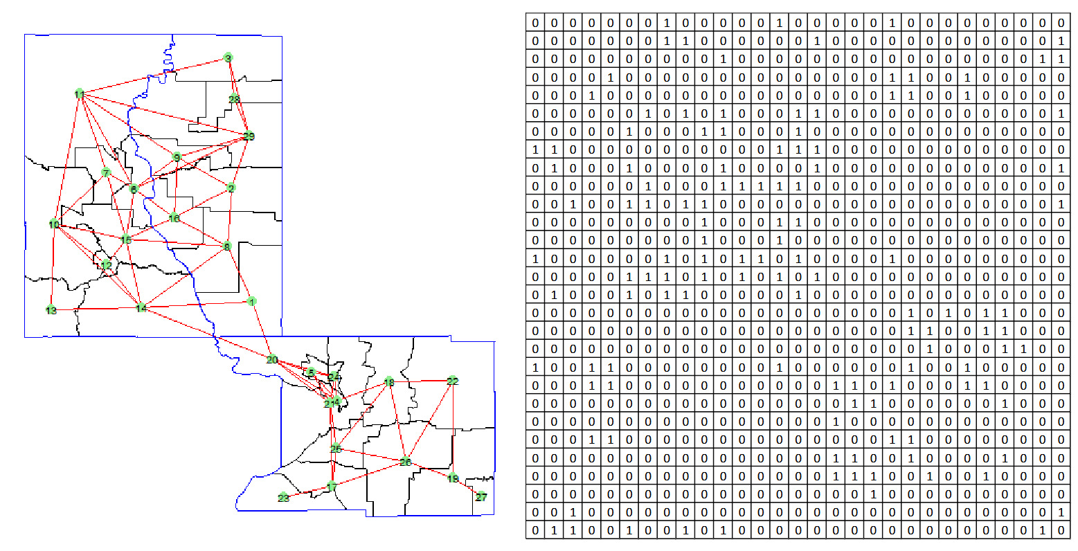
The adjacency matrix \(A\) captures these connections with \(a_{ij} = 1\) if tracts \(v_{i}\ and\ v_{j}\) are adjacent, and \(a_{ij} = 0\) otherwise. Notably, this adjacency matrix is symmetric, as adjacency between tracts is mutual; if \(v_{i}\) is adjacent to \(v_{j}\), then \(v_{j}\) is also adjacent to \(v_{i}\). The rationale behind this approach is that census tracts in close geographical proximity are likely to share similar characteristics, such as socioeconomic factors, infrastructure, and environmental conditions, which could result in comparable risk measures. Figure 2 demonstrates the graph constructed using this method, where each node (census tract) is connected to its adjacent nodes. The adjacency matrix corresponding to this graph clearly indicates whether two nodes are geographically adjacent. The main advantage of this method lies in its simplicity: The only required information is whether two census tracts are geographically adjacent. However, this simplicity can also become a limitation. When the number of adjacent nodes is large, the graph can become highly complex, with numerous connections. Additionally, this method does not account for the size of each census tract; adjacency alone determines proximity, which may not always reflect the true geographical influence between tracts.

Figure 2.Left: Graph based on geographical adjacency. Right: Corresponding adjacency matrix.

2.1.2. Geographical proximity

To better measure geographical proximity while controlling the complexity of the graph, we introduce a more refined approach using the K-nearest neighbors (KNN) method. This approach allows for a controlled and scalable construction of the graph, focusing on local proximity while managing the overall number of edges. The process of creating such a graph is described below.

• Calculate the distance matrix: Compute the pairwise distances between all nodes, resulting in a distance matrix \(D = \left\lbrack d\left( v_{i},\ v_{j} \right) \right\rbrack_{i,j}\), where \(d\left( v_{i},\ v_{j} \right)\) represents the distance between nodes \(v_{i}\) and \(v_{j}\). For geographical data, nodes are defined by geographic centroids, and the haversine distance is commonly used to calculate the distance between two points on the Earth’s surface, given their latitudes and longitudes:

  \(\scriptsize d\left( v_{i},\ v_{j} \right) = 2r \times \arcsin\left( \sqrt{\sin^{2}{\left( \frac{\phi_{j} - \phi_{i}}{2} \right) + \cos{\left( \phi_{i} \right)\cos\left( \phi_{j} \right)\sin^{2}{\left( \frac{\lambda_{j} - \lambda_{i}}{2} \right)}}}} \right)\),

  where \(\phi\) is latitude, \(\lambda\) is longitude, and \(r\) is the Earth’s radius.

• Identify K-nearest neighbors and construct graph: For each node \(v_{i}\), identify its K-nearest neighbors based on the distance matrix D. Then, form an edge \(e_{ij}\) between node \(v_{i}\) and each of its K-nearest neighbors \(v_{j}\), such as

  \(E = \left\{ e_{ij} = \left( v_{i},\ v_{j} \right)\ |\ v_{j} \in \ \mathcal{N}_{K}\left( v_{i} \right) \right\}\),

  where \(\mathcal{N}_{K}\left( v_{i} \right)\) denotes the set of K-nearest neighbors of node \(v_{i}\).

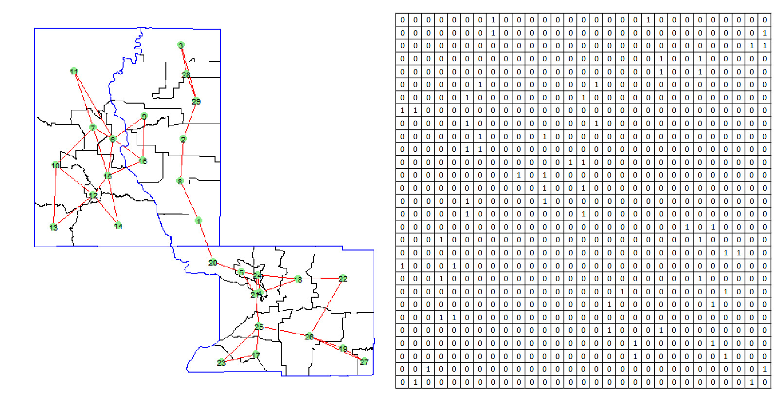
Figure 3 illustrates the graph generated with \(K = 2\) and the corresponding adjacency matrix. Unlike the previous adjacency approach, the adjacency matrix \(A\) in this method reflects only the K-nearest neighbors rather than immediate geographical adjacency. Specifically, \(a_{ij} = 1\) if tract \(v_{j}\) is among the K-nearest neighbors of tract \(v_{j}\), and \(a_{ij} = 0\) otherwise. Consequently, the adjacency matrix in this case is generally asymmetric, as proximity is not necessarily mutual: \(v_{j}\) may be a nearest neighbor to \(v_{i}\), while \(v_{i}\) may not be among the K-nearest neighbors of \(v_{j}\). The KNN method provides an effective means of constructing a graph that emphasizes local spatial relationships among census tracts. By controlling the number of neighbors, this approach strikes a balance between capturing meaningful spatial dependencies and limiting graph complexity, which can be particularly useful when dealing with large datasets.

Figure 3.Left: Graph based on geographical proximity. Right: Corresponding adjacency matrix.

2.2. Graph node embedding

To effectively learn the representation of each node in the previously constructed graph, we employ a graph embedding technique. Given a graph \(G(V;E)\), the goal of graph embedding is to develop a mapping function \(f:v_{i} \mapsto \mathbf{y}_{v_{i}} \in \mathbb{R}^{d},\) where \(d \ll |V|\), that maps each node \(v_{i}\) to a vector \(\mathbf{y}_{v_{i}}\) in a lower-dimensional space, aiming to preserve the similarity between the embeddings of nodes based on their proximity in the graph. This preservation includes both first-order proximity (direct connections between nodes) and second-order proximity (similar nodes being connected to the same neighbors), as outlined in studies by Wang et al. (2016) and Makarov et al. (2021).

To generate vector representations of nodes, we use the Node2Vec approach (Grover and Leskovec 2016). Inspired by the skip-gram model (Mikolov et al. 2013), Node2Vec treats a graph similarly to a “document,” where nodes sampled in sequences from the graph resemble words in an ordered sequence. Formulated as a maximum likelihood optimization problem, Node2Vec seeks to learn an embedding function \(f:V \mapsto \mathbb{R}^{d}\), where d represents the dimensionality of the embeddings. This function can be viewed as a matrix of size |\(V| \times d\). For every source node \(v \in V\), we define \(\mathcal{N}_{S}(v) \subset V\) as a neighborhood of node \(v\), generated through a specific neighborhood sampling strategy S.

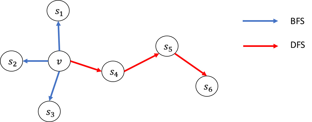
Node2Vec leverages a unique biased random walk mechanism to achieve a flexible neighborhood search strategy and include parameters that allow for tuning the explored search space. Consequently, for a given source node \(v\), the neighborhoods \(\mathcal{N}_{S}(v)\) are not limited to direct neighbors but can include nodes from more varied structures. Searching neighborhoods can be seen as a form of local search. Figure 4 illustrates a source node v where different search strategies generate different neighborhoods \(\mathcal{N}_{S}(v)\). For comparative purposes, the size of the neighborhood \(\mathcal{N}_{S}(v)\) is constrained to \(M\) nodes, and multiple sets can be sampled for a single node \(v\). There are two primary search strategies for generating neighborhood sets \(\mathcal{N}_{S}\) of size \(M\):

• Breadth-first search (BFS). This strategy restricts the neighborhood \(\mathcal{N}_{S}\) to the immediate neighbors of the source node. For example, in a scenario where \(M = 3\), BFS might sample nodes \(s_{1},s_{2},s_{3}\) directly connected to \(v\).

• Depth-first search (DFS). In contrast, this strategy samples nodes sequentially at increasing distances from the source node. For instance, DFS could yield nodes \(s_{4},s_{5},s_{6}\) that are further away from \(v\).

These two search methods represent extreme ends of the search space they explore, which can significantly influence the resulting node representations.

Figure 4.BFS and DFS search strategies from node \(v\) for \(M = 3\).

Node2Vec employs a biased random walk to facilitate transitions between the BFS and DFS strategies. For each node \(v \in V\), we generate a random walk \(U_{v} = (u_{1},u_{2},\ldots,u_{l})\) of length \(l\) with \(u_{1} = v\), and \(u_{i} \in V\), for \(i = 2,\ldots,\ l\). The unnormalized transition probability from node \(u_{i}\) to node \(u_{j}\) is given by

\(\pi_{u_{i}u_{j}} = \alpha \cdot w_{u_{i}u_{j}}\),

where \(w_{u_{i}u_{j}}\) is the edge weight, and \(\alpha\) is defined as

\(\alpha= \begin{cases}\frac{1}{p} & \text { if } d_{u_{i-1} u_j}=0 \\ 1 & \text { if } d_{u_{i-1} u_j}=1 \\ \frac{1}{q} & \text { if } d_{u_{i-1} u_j}=2\end{cases}.\)

Here, \(d_{u_{i - 1}u_{j}}\) denotes the shortest path distance between nodes \(u_{i - 1}\) and \(u_{j}\). The transition probability is controlled by two hyperparameters: the return parameter \(p\) and the in-out parameter \(q\). The parameter 𝑝 controls the likelihood of revisiting nodes, enabling the walk to remain close to the starting point; a smaller \(p\) favors depth-first exploration. Conversely, parameter \(q\) governs the probability of venturing outward, with a smaller \(q\) promoting broader exploration akin to BFS. By adjusting \(p\) and \(q\), Node2Vec can effectively balance exploration and exploitation, adapting the random walk to fit the specific structural nuances required by the application. This adaptability allows Node2Vec to effectively capture both homophily—where similar nodes are connected—and structural equivalence, which refers to the interconnection of nodes performing similar roles.

To compute embeddings \(\mathbf{y}_{v_{i}}\), for, \(i \in \{ 1,\ldots,\ |V|\}\), Node2Vec extends the skip-gram architecture to graphs (see Perozzi et al. 2014; Mikolov et al. 2013) by maximizing the probability of observing a neighborhood node given a source node. The objective function is expressed as follows:

\[\max\sum_{v \in V}{\sum_{u_{i} \in U_{v}}{\sum_{u_{j} \in \mathcal{N}_{S}(u_{i})}{\log{P\left( u_{j} \right|u_{i})}}}}\ .\]

The probability \(P\left( u_{j} \right|u_{i})\) is defined following the skip-gram model:

\[P\left( u_{j} \right|u_{i}) = \frac{exp(\mathbf{y}_{u_{j}}^{T}\mathbf{y}_{u_{i}})}{\sum_{v \in V}{exp(\mathbf{y}_{v}^{T}\mathbf{y}_{u_{i}})}}\ .\]

The optimization problem is solved using stochastic gradient descent along with negative sampling, which approximates the softmax function by considering only a limited number of negative samples for each positive example.

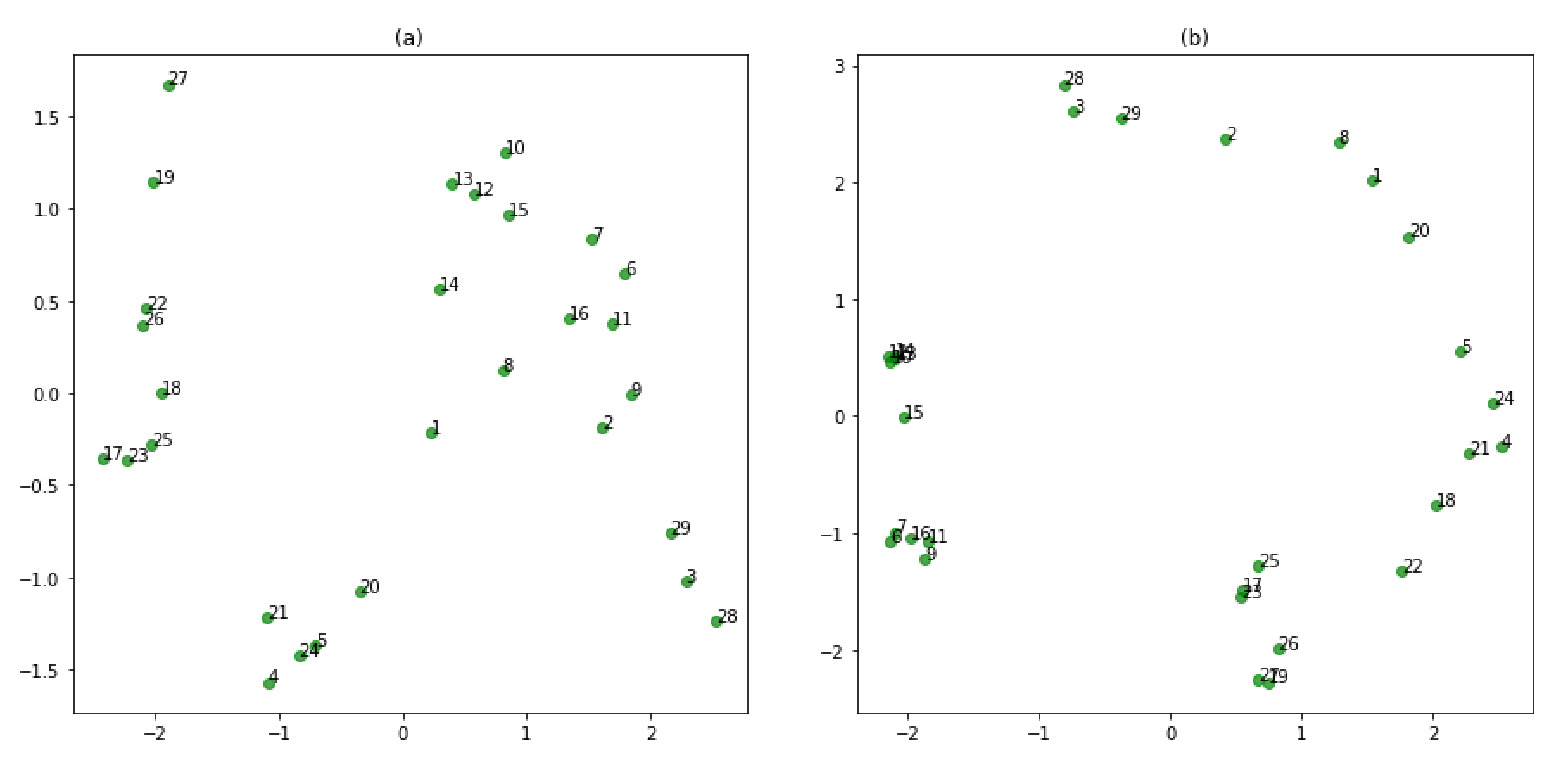
For the graphs illustrated in Figure 2 and Figure 3, we employ Node2Vec to generate node embeddings of size 3 for each census tract by conducting random walks of length \(l = 20\). To visualize the embeddings, we apply principal component analysis (PCA) to reduce dimensionality and plot the embeddings along the first two principal components, as illustrated in Figure 5. The results demonstrate the effectiveness of these embeddings in capturing geographical relationships, leading to the following key observations:

• Geographical adjacency: The embeddings show minimal clustering effects. In the PCA plot, the points representing geographically adjacent census tracts are positioned closer together, accurately reflecting the local neighborhood structures. This indicates that the embeddings successfully encode adjacency information, allowing tracts near each other in space to remain near each other in the embedding space, but without forming distinct clusters.

• Geographical proximity: The embeddings display stronger clustering. This method incorporates a KNN approach, imposing additional structure by limiting node connections to their closest neighbors. This results in the formation of subgraphs, which are apparent in the PCA plot. For example, nodes 6, 7, 9, 11, and 16 are isolated from other nodes, forming distinct clusters separated from the rest. This method highlights how embeddings can capture local but constrained proximity, producing separate clusters that represent smaller, isolated groups within the larger geography.

These observations demonstrate that Node2Vec embeddings effectively preserve and reflect underlying geographical and hierarchical relationships among census tracts. Each method emphasizes different spatial or structural aspects of the data, from local adjacency to broader hierarchical boundaries, allowing for flexible exploration of geographical information within the embeddings.

Figure 5.PCA visualization of the graph node embeddings with graph constructed using (a) geographical adjacency and (b) geographical proximity.

2.3. Discussion

Scalability. Our method leverages the Node2Vec framework for node embedding, which is well suited for large-scale graphs due to its efficient and scalable design (Grover and Leskovec 2016). Node2Vec uses biased second-order random walks with precomputed alias sampling, allowing each step in the walk to be performed in constant time after preprocessing. The overall time complexity for walk generation is \(O(|V| \cdot r \cdot l)\), where \(|V|\) is the number of nodes in the graph, \(r\) is the number of walks per node, and \(l\) is the length of each walk. In practice, both \(r\) and \(l\) are treated as fixed hyperparameters, ensuring that the walk generation process scales linearly with the number of nodes. The subsequent embedding optimization relies on the skip-gram model with negative sampling (Mikolov et al. 2013), which also exhibits linear time complexity with respect to the number of training pairs. These design choices allow our method to scale effectively to graphs with millions of nodes and edges, while maintaining computational efficiency and manageable memory requirements.

Hyperparameter tuning. Node2Vec introduces four main hyperparameters that influence the quality and behavior of the learned node embeddings: the number of walks per node (\(r\)), the length of each walk (\(l\)), and the walk bias parameters \(p\) and \(q\). Based on empirical studies and our experience, we suggest the following practical guidelines. First, setting \(r = 200\) and \(l = 5\) provides a strong baseline and works well across a wide range of graph sizes and domains. Increasing these values may improve embedding quality but comes with higher computation cost. Second, the parameters \(p\) and \(q\) control the walk’s bias between BFS and DFS exploration. To capture homophily (nodes connected to similar nodes), a lower \(q\) (e.g., \(q < 1\)) encourages BFS-like behavior and is typically effective. To capture structural roles (nodes playing similar functions regardless of connection), a higher \(q\) (e.g., \(q > 1\)) induces DFS-like behavior and tends to perform better. The parameter \(p\) can usually be set to 1 unless there is a specific need to encourage or discourage walk backtracking. In practice, we recommend grid searching over a small set of values (e.g., \(p \in \{ 0.25,1,2\},\ q \in \{ 0.25,1,2\}\)) using downstream validation performance as a guide.

3. Applications of knowledge-based embedding

In this section we demonstrate the application of our proposed embedding method in two key use cases. Section 3.1 describes the dataset used for the analysis, Section 3.2 visualizes the embedding results, and Sections 3.3 and 3.4 present the method’s effectiveness in addressing two critical challenges: (1) generating robust risk classifications for high-cardinality categorical variables, and (2) deriving reliable embeddings for new categories with no prior historical data.

3.1. Data description

The dataset used for our analysis is obtained from Commonwealth Automobile Reinsurers (CAR) in Massachusetts, United States. CAR serves as both the residual market and the statistical agent for motor vehicle insurance in the state, tasked with collecting, editing, and processing premium and claims data for private passenger and commercial automobile insurance policies. For a more detailed discussion on the dataset, see Shi and Shi (2017).

Our analysis focuses on claims data from personal automobile insurance policies in the year 2006. For simplicity, we limit our analysis to policyholders with full-year exposure. For each policyholder, the dataset records whether a claim was filed during the year. In addition to the claims data, the dataset provides several key pricing variables insurers typically use, offering insights into the characteristics of both the driver and the insured vehicle. Specifically, policyholder information is limited to the primary driver’s age group, which is categorized into three groups: young, adult, and senior. Vehicle characteristics include vehicle age, vehicle type (categorized as passenger car, van, pickup truck, or utility vehicle), whether the vehicle is classified as luxury, and whether it has all-wheel drive. Furthermore, the dataset contains geographic information related to the vehicle’s garage location, represented by the town where the vehicle is garaged, which is a crucial variable in risk assessment and pricing.

Table 1 presents detailed descriptions and summary statistics for these variables. The data show that approximately 5% of policyholders experienced at least one accident during the year, indicating a relatively low frequency of claim events within the dataset. Additionally, young drivers make up 10% of the sample, adult drivers 75%, and senior drivers 15%. The average vehicle age is around five years, with 5% classified as luxury cars. Most vehicles are passenger cars, and 35% have all-wheel drive.

The analysis focuses on claim frequency. In this dataset, only about 0.19% of policyholders had more than one accident during the year. Given the low proportion of multiple claims, we use logistic regression to model the likelihood of claim occurrence.

3.2. Categorical embedding

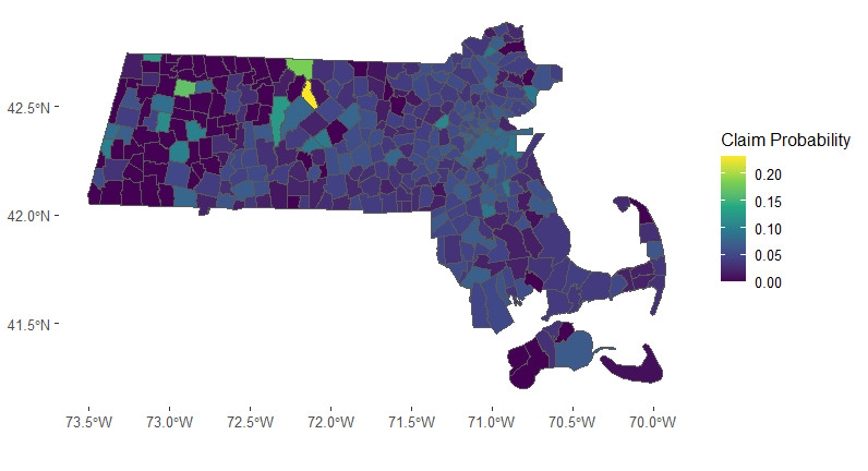
The state of Massachusetts comprises a total of 351 towns. In Figure 6, we present a heatmap illustrating the town-level probability of insurance claims. The map reveals distinct spatial clusters in claims frequency, particularly evident in the Boston area and the far southeastern region of the state. The spatial clusters suggest potential groupings of towns for more effective risk assessment and management.

Figure 6.Heatmap of auto claim probabilities across towns in Massachusetts.

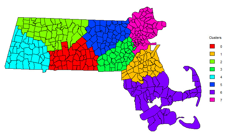
To generate embedding vectors for the town variable, we employed the knowledge-based embedding approach described in Section 2. For illustration, we constructed a graph using the geographical proximity method, establishing connections between each town and its two nearest neighbors. Subsequently, we generated embeddings of size 10 for each town. Using the resulting categorical embeddings, we conduct a cluster analysis with the K-means algorithm. The elbow method is employed to identify the optimal number of clusters. We determine that eight town clusters provide the best representation of the data, which are further visualized in Figure 7. This clustering allows us to group towns with similar risk characteristics, facilitating targeted strategies for insurance pricing and claims management.

Figure 7.Graphical representation of town clusters generated from the learned embeddings.

3.3. Risk classification

In the first application, we explore the role of our knowledge-based embedding method in risk classification, a core actuarial function essential to underwriting and ratemaking. In this process, insurers identify rating factors that can effectively segment policyholders into homogeneous classes based on similar risk characteristics. Within these classes, policyholders exhibiting similar risk profiles are charged comparable premiums for equivalent coverage, ensuring equitable and consistent pricing.

Our focus is on classifying risk for policyholders across diverse geographic regions in Massachusetts, in addition to other relevant predictors. Given that there are 351 towns in Massachusetts, it’s reasonable to assume that not all towns present distinct risk profiles. Additionally, risks may exhibit spatial dependence, meaning that drivers in adjacent towns may have correlated latent risk factors, while drivers in towns further apart may not. Therefore, our analysis aims to segment policyholders into meaningful risk clusters, leveraging geographical location as a crucial input in identifying these nuanced clusters.

To illustrate the application of our generated geographical clusters, we conduct both in-sample and out-of-sample analyses. The dataset is split randomly into a training set and a test set, with stratified sampling based on town names, 80% of observations allocated to the training set, and the remaining 20% to the test set. Using the training data, we fit two logistic regression models. The first model incorporates only policy-related information from Table 1, while the second model builds on that information by including the geographical clusters as an additional categorical predictor. Estimated parameters for both models are reported in Table 2. Two significant insights emerge from this comparison. First, the geographical clusters derived from our embedding method display statistically significant effects in the second model, underscoring the predictive value of location-based information. Second, comparing the regression coefficients for shared rating variables across the two models, we observe that incorporating geographical clusters influences the estimates for these variables, indicating that rating variables are partially town-dependent.

To further validate the effectiveness of our knowledge-based embedding method in synthesizing information within the town categorical variable, we assess the model performance in both goodness of fit for the training data and prediction accuracy for the test data across four different modeling approaches. The baseline model is a logistic regression without town-specific information. The remaining models incorporate town data in three different ways: (1) one-hot encoding for each town, (2) direct embeddings for each town generated by our proposed method, and (3) town clusters derived from the learned embeddings. The results are summarized in Table 3 for the training data and Table 4 for the test data.

Table 3 presents the goodness-of-fit metrics—area under the curve (AUC), log-likelihood score, Akaike information criterion (AIC), and Bayesian information criterion (BIC)—for the training data across the four models. Models incorporating geographical information, especially one-hot encoding, demonstrate higher AUC and log-likelihood scores, indicating an improved fit when town information is considered. However, when model complexity is factored in, the models with geographical data, particularly one-hot encoding, show less favorable AIC and BIC values due to the higher number of parameters. Thus, while one-hot encoding may enhance fit, it also introduces a risk of overfitting due to its high dimensionality.

Table 4 compares prediction accuracy on the test data across the four models, reporting AUC, Gini index, and Pearson and Spearman correlation coefficients. Two key findings emerge from this analysis. First, across all accuracy metrics, models with geographical data outperform the baseline model, reaffirming the relevance of geographic information in risk classification. Second, while one-hot encoding shows better goodness of fit in the training data, it performs comparably to or even worse than our embedding-based models on test data metrics. This suggests potential overfitting in the one-hot encoding approach, likely due to the high number of parameters compared to the more parsimonious and structured embedding approach we propose.

To summarize, our method successfully captures the latent relationships among regions, generating risk clusters that are both interpretable and aligned with industry expectations. These clusters allow insurers to categorize policyholders more precisely, enabling more accurate premium pricing and improving risk management decisions. The method’s ability to identify nuanced risk patterns that may not be immediately apparent in the raw data demonstrates its practical utility in underwriting and actuarial modeling.

3.4. Pricing new risks

In the second application, we address the challenge of pricing risks in a newly entered geographical region where historical insurance data may be unavailable. This scenario is especially relevant for insurers seeking to expand into unfamiliar markets or regions with limited prior data. To demonstrate the applicability of the proposed method, we split the dataset into two parts based on geographic location rather than a random assignment of observations. Specifically, we randomly select 300 towns and use all observations within those towns as the training data, while observations from the remaining towns constitute the test set. This setup ensures that the test data include towns previously unseen in the training data, simulating the scenario of an insurer developing rating strategies for newly expanded areas using historical data from a set of familiar regions.

To initiate the analysis, we fit two logistic regression models to predict the binary claim outcome. The first model incorporates only basic rating variables, while the second model includes both basic rating variables and additional predictors derived from the town clusters generated through our knowledge-based embedding approach. We present the estimated parameters for both models in Table 5, where we observe that the town clusters exhibit statistically significant effects on claim frequency. Moreover, incorporating the town clusters also affects the relativities of other rating variables, highlighting the interdependencies among rating factors. However, in contrast to the first application, some towns in this setup are entirely new to the insurer, lacking any historical claim data. This means that relativities for town-based risk classifications cannot be directly inferred from past data, making traditional approaches, such as one-hot encoding for town categories, unsuitable.

To validate the predictive power of the learned town embeddings, we compare models with and without those embeddings in terms of both goodness of fit for the training data and prediction accuracy for the test data. Tables 6 and 7 summarize the results, using the same metrics as in the first application. Here, we evaluate both the direct use of learned embeddings and the indirect use of town clusters within logistic regression. Notably, one-hot encoding for towns, as used in the first application, is not feasible because the test data include towns unobserved in the training data.

The results reveal that models incorporating town information—either through direct embeddings or through clusters—demonstrate comparable, if not superior, goodness of fit compared to the baseline model without town information. In the test data, which contains previously unseen towns, models with embedded town information show improved risk classification and prediction accuracy, underscoring the value of incorporating geographic data for forecasting risk in unfamiliar regions. Interestingly, the town clusters appear to capture the essential information from the direct embeddings without significant loss, as indicated by favorable out-of-sample prediction metrics. Additionally, town clusters offer enhanced interpretability, providing insights into the spatial structure of risk that can be particularly useful for practical decision-making.

In summary, by leveraging the inherent relationships between geographical regions, our method provides a reliable framework for estimating risk for previously unseen areas. Specifically, the graph-based embedding technique allows us to infer risk characteristics for the new region by drawing on its connections to existing regions with known risk profiles. As a result, our method produces risk estimates that are both interpretable and grounded in the spatial structure of the data, offering a robust solution for pricing risks in uncharted territories.

4. Conclusion

In this paper, we introduced a knowledge-driven embedding approach tailored for high-cardinality categorical variables in actuarial applications. By constructing graph representations that encode domain-specific relationships and applying graph neural embedding techniques, we demonstrated how complex categorical structures, such as geographical or hierarchical data, can be captured and leveraged in insurance models. Our proposed method enhances the representation of categorical variables, encapsulating latent patterns and relationships that traditional methods—such as one-hot encoding or existing embeddings—often overlook.

Through empirical studies using a real-world automobile insurance dataset, we illustrated the practical impact of this approach in two critical scenarios: risk classification for high-cardinality variables and risk pricing in new, unseen geographical areas. In both cases, our approach not only improved predictive accuracy but also added interpretability to the results, making it a powerful tool for actuaries in modeling nuanced risk factors. The method’s ability to generalize to new regions based on spatial and relational patterns also highlights its relevance for insurers entering new markets with limited historical data, addressing a common challenge in expanding insurance operations.

The results of this study underscore several key advantages of our knowledge-based embedding approach. First, it provides a robust alternative to conventional embeddings by retaining intricate domain-specific insights, thereby yielding richer and more relevant representations. Second, the graph-based nature of the method allows for interpretable risk clusters, helping insurers not only predict risk but understand the relationships between categories—an added benefit in regulatory and operational contexts. Finally, our work contributes to the broader field of predictive modeling in actuarial science by introducing a scalable method that aligns with the industry’s growing reliance on data complexity and diversity.

Looking ahead, our method offers a promising foundation for extending categorical feature construction to other domains within actuarial science, such as claims reserving and fraud detection. Future research could explore its adaptability to other categorical types, such as policyholder demographics or coverage options, potentially leading to comprehensive risk assessment frameworks that further enhance the precision of insurance pricing strategies. By integrating complex, unstructured categorical data into actuarial models, we believe this approach paves the way for more robust, insightful, and adaptable predictive modeling in the insurance industry.