Using Large Language Models to Generate New Features from Text Data for Loss Prediction

1. Introduction

Text data are unstructured data that are stored and written in text format. Insurance companies collect an enormous amount of text data from multiple sources such as customer feedback, claims adjuster notes, underwriter notes, accident descriptions, etc. Text data provide more context than numerical data and can be analyzed to extract valuable insights.

Several methods are available for analyzing text data. One method applies pretrained language models, which can be used for a number of traditional natural language tasks, including summarization, sentiment analysis, etc. Table 1 shows a timeline of language model development over the past three decades as they progressed through four major stages, from the initial statistical language models to the current stage of large language models (LLMs). Statistical language models use probability distributions to model word sequences. Neural language models use neural networks to capture complex patterns and representations of language. Pretrained language models use large corpora and self-supervised learning to capture general linguistic knowledge. LLMs extend pretrained language models by processing massive amounts of data.

LLMs are language models (LMs) with massive parameter sizes that have exceptional capabilities to understand and generate human language (Chang et al. 2024). LLMs are built using deep learning techniques, are trained on vast amounts of text data, and can perform a variety of natural language processing tasks, such as text generation, translation, summarization, and question answering. LLMs have been applied in various fields, such as software engineering, computational biology, medicine, law, and education, to name just a few. Well-known LLMs include OpenAI’s GPT-3 and GPT-4, Google’s BERT, and Meta’s Llama 1 and Llama 2. Wang et al. (2024) and Raiaan et al. (2024) have conducted comprehensive surveys of LLMs.

Two paradigms are used to apply pretrained LMs (Liu et al. 2023), (1) the pretrain and fine-tune paradigm, and (2) the pretrain, prompt, and predict paradigm. In the first, a pretrained LM is fine-tuned for downstream tasks with objective functions including additional parameters. This paradigm focuses on objective engineering that consists of designing the training objectives used at both the pretraining and fine-tuning stages. In the second paradigm, a pretrained LM is used for downstream tasks directly with the help of textual prompts. This paradigm focuses on prompt engineering that reformulates downstream tasks to look like those solved during the original LM training.

Our research investigated the use of pretrained LLMs to create features from text data with the help of textual prompts and studied the effectiveness of incorporating such features for predicting insurance losses. Our method has the following advantages: first, using pretrained LMMs circumvents a supervised learning condition, which requires large sets of labeled text data; second, the features produced by pretrained LLMs have lower dimensions than those produced by traditional text analysis techniques such as topic modeling; third, pretrained LLMs can understand complex texts and concepts in different languages through their analytical and machine translation capabilities.

The remainder of the paper is organized as follows. Section 2 provides a brief review of existing approaches to text data analysis as applied to insurance analytics and discusses potential applications of LLMs. Section 3 describes the public dataset containing the text descriptions that provided the basis for our study. Section 4 introduces the principles of prompt engineering. Section 5 presents the numerical results obtained by applying two LLMs to the dataset. Finally, Section 6 provides a summary and closing remarks.

2. Literature Review

Researchers in the actuarial community have used text data in their studies. For example, text mining techniques, from topic modeling to vector embeddings, have been used to analyze text data in the insurance setting (Liao et al. 2019; Baillargeon et al. 2020; Zappa et al. 2021; Manski et al. 2021). While many studies have analyzed text data with traditional natural language processing (NLP) methods, the use of LLMs has been limited. This section provides a brief summary of the text-related explorations that have been published, as well as a foray into LLMs where applications exist.

Lee et al. (2019) considered how to enhance insurance analytics using textual data via the concept of word similarities. Word or sentence embedding models provide numerical representation of text data that retains semantic meaning. In the context of property insurance, for example, the embedding vector of a word like “fire” will be closer to the embedding of a word like “arson” than it will be to a word like “theft.” Actuarial applications can benefit from this encoding scheme. Lee et al. (2019) leveraged this approach by defining a procedure for extracting new numeric variables from text data and incorporating them into claims analytics. The authors demonstrated that the ability of models to predict and quantify risk is enhanced through the use of NLP methods.

Liao et al. (2019) investigated customer service practices of US personal lines insurance carriers using a variety of techniques, including word clouds, latent Dirichlet allocation for topic modeling, and a selection of pretrained sentiment analysis algorithms. Their study was an exploratory unsupervised analysis, demonstrating the potential for text data to enhance analytical capabilities in the actuarial space. The authors’ core finding was that unsupervised analysis of text data can identify frequent call topics, how customer sentiment differs between calls, and other factors in a highly automated fashion.

In the supervised analysis setting, Baillargeon et al. (2020) expanded the focus beyond traditional statistical actuarial models by exploring the potential of using neural architectures with unstructured text data to mine risk predictors from accident descriptions. The authors used features identified as important for assessing the underlying relationships as inputs to a Poisson regression model, from which they estimated the number of cars involved in an accident using the text description of the accident itself. In a similar setting, Zappa et al. (2021) used text narratives of accident occurrences from the US National Highway Traffic Safety Administration to extract semantic information that can be used in a regression context for fine-tuning premium decisions.

Manski et al. (2021) used text descriptions from a property claims dataset to predict risk. Using Word2Vec to condense the text descriptions into dense embeddings, they used a nonlinear transformation of the captured embeddings as inputs to a gamma double generalized linear model (GLM) (Smyth and Verbyla 1999) that regularizes for mean and dispersion. These studies demonstrate strong potential for using NLP techniques to supplement the rating and risk-determination process, but none of the models leverage LLMs.

Balona (2024) focused specifically on LLMs, aiming to summarize the existing and potential use cases for LLMs in actuarial work. The author defined the contributions of LLMs as directly beneficial to actuarial work as well as helping to make the process more efficient. Further, the author provided guidelines for when LLMs should be considered for actuarial work, considering factors such as data structure (e.g., if the data are highly structured and numeric, traditional approaches may be more suitable). The author noted that LLMs are technically best when the data are less structured, require context and pattern recognition, and/or require the generation of new content.

Li et al. (2025) proposed a comprehensive framework for examining discrepancies in textual content using LLMs. The authors focused on using the OpenAI interface to embed text and project it into categories, using distance metrics to evaluate discrepancies. The approach is based on three types of relationships: identical information, logical relationships, and potential relationships.

Some research on using LLMs to generate new features for predictive models exists outside the insurance field. Malberg et al. (2024) proposed an approach to use pretrained LLMs to generate a set of human-interpretable features from text data. Their methodology generates human-interpretable features and outperforms traditional methods like term frequency-inverse document frequency (Salton and Buckley 1988) and vector embeddings. Hollmann et al. (2023) proposed an automated feature development method by using LLMs to iteratively generate meaningful features for tabular datasets.

Text embeddings play a central role in transforming unstructured text into numerical representations suitable for modeling and analysis. One of the earlier approaches—the term frequency-inverse document frequency (Salton and Buckley 1988)—represents documents using sparse vectors that capture word occurrence patterns; however, it lacks semantic meaning. Subsequent developments introduced static word embeddings, such as Word2Vec (Mikolov et al. 2013) and GloVe (Pennington et al. 2014), which learn dense vector representations based on word co-occurrence statistics and encode semantic relationships between words. However, these embeddings are context-independent, assigning the same vector to a word regardless of its usage. The introduction of contextual embeddings, such as Bidirectional Encoder Representations from Transformers (BERT) (Devlin et al. 2019), addressed this limitation by generating dynamic representations that vary with surrounding text, enabling more accurate capture of linguistic nuance. Modern LLMs extend these ideas further—their deep transformer architectures produce high-dimensional embeddings that encode not only local syntax and semantics but also broader conceptual and relational information.

3. Description of the data

We used data from the Wisconsin Local Government Property Insurance Fund (LGPIF) for this study. The LGPIF was created to provide insurance to government properties not owned by the state of Wisconsin. The program made insurance available for local government properties like municipal buildings, schools, libraries, vehicles, etc. The dataset includes claims collected from 2006 to 2010 as a training set ($n$ = 4,991) and claims from 2011 as a test set ($n$ = 1,039).^[1] The dataset includes nine binary variables (Vandalism, Fire, Lightning, Wind, Hail, Vehicle, WaterNW, WaterW, and Misc), one text variable (Description), and a continuous variable (Loss).

The LGPIF dataset has been used extensively in actuarial literature. Frees et al. (2016) used it for a case study that extends the literature on multivariate frequency-severity regression using copulas. The data have also been used to propose a multivariate framework for pricing property insurance contracts with multiperil coverage using a two-part model with heavy tails and Gaussian copulas (Yang and Shi 2018). A similar assessment is presented by Lee and Shi (2019). In another study, Lee et al. (2019) conducted a text-based analysis of the same dataset using the concept of word similarities to generate new features for regression modeling. The authors used the pretrained GloVe word embeddings framework to convert words in the LGPIF dataset claims descriptions into semantic embedding vectors. To extract features for modeling, they computed the cosine similarity between these word vectors and a curated set of keywords representing claims-related concepts (e.g., vandalism, fire, etc.). The similarity scores were fed into generalized additive models and GLMs to develop models that retain semantic information from text in the loss prediction framework.

Manski et al. (2021) used the LGPIF text data to predict loss amounts by applying a gamma double GLM approach. The authors first used GloVe to create sentence-level embeddings of each claim description by averaging the GloVe vectors of all words in the sentence. Next, they applied principal component analysis to the average embeddings and retained the first 10 principal components as summary features of the text. The 10 principal components were fed into a gamma double GLM model, which included a mean component (for expected loss) and a dispersion component (for variance), both modeled as functions of the text-derived features. Their analysis showed that text features significantly improve predictive performance and interoperability.

Other applications of the dataset include diagnostic testing (Li et al. 2023), dependency modeling (Lee 2023), hazard type prediction (Wüthrich and Merz 2023), and auto machine learning (Dong and Quan 2025). We identified a number of slight variations in the dataset across these sources and focused in particular on the property insurance claims across different loss types, as in Manski et al. (2021), with a particular focus on the text descriptions of claims.

Tables 2(a) and 2(b) provide a summary of the loss by category for the training set and the test set, respectively. The categories are sorted by the average loss. From the two tables, we see that hail caused the highest loss and fires caused the second highest loss. However, the average loss ranks of other categories differ for the training and test sets.

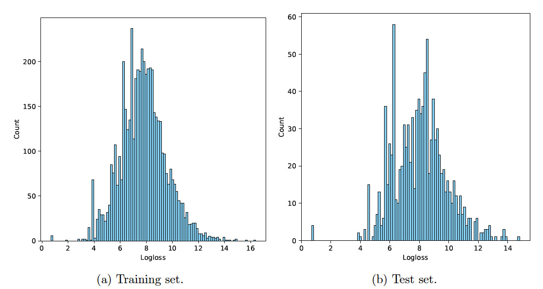
The summary statistics shown in Table 2 show that the loss variable is highly skewed because the overall mean is several times greater than the third quantile. Figures 1(a) and 1(b) show the histograms of the log-transformed loss for the training set and the test set, respectively. Let $Y$ denote the loss variable. The logloss shown in the histograms is calculated by $\ln(1+Y)$. The histograms show that the log-transformed loss is much less skewed. Since the log-transformed loss is positive, gamma distributions can be used to fit the data.

For these analyses, we were most interested in the text descriptions of each claim. Table 3 summarizes the textual characteristics of the training and test datasets. The training set contains 22,759 total words, roughly four times the 5,057 words in the test set, with 2,090 and 1,006 unique words, respectively. Both datasets have similar linguistic patterns, with an average word length of about 6.3 characters and an average of approximately four to five words per description. The proportion of stopwords is also consistent across the two sets, around 17%–18%. Measures of lexical diversity show some variation: Yule’s $K$ is higher for the training set (258.9) than for the test set (128.9), indicating greater repetition of words, while Herdan’s $C$ is slightly lower in the training set (0.76 vs. 0.81), consistent with a more diverse vocabulary in the smaller test sample. Yule’s $K$ (Tweedie and Baayen 1998; Yule 2014) measures vocabulary repetitiveness, with larger values indicating less lexical diversity, whereas Herdan’s $C$ (Herdan 1960) quantifies lexical richness on a scale between 0 and 1, where higher values represent a more varied vocabulary. Overall, the statistics suggest that the two datasets are comparable in linguistic structure, with minor differences in lexical richness and word repetition.

Figure 1.Histograms of the log transformed loss.

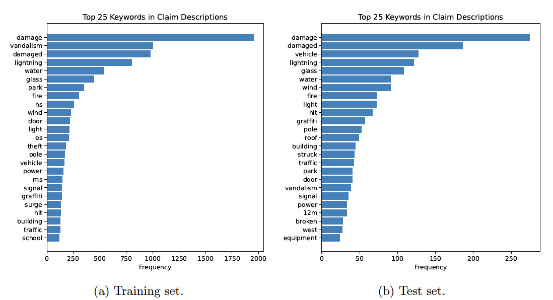
Figures 2(a) and 2(b) show the top keywords extracted from the claim descriptions in the training set and the test set, respectively. The top keywords are selected based on their frequency of occurrence in the incident descriptions. For example, the word “damage” appears about 2,000 times in the incident descriptions of the training set. As shown in the two figures, the sets of top keywords from the training set differ from those of the test set. However, the first keyword (i.e., damage) is the same for both the training set and the test set.

Figure 2.Distribution of common keywords in claim descriptions.

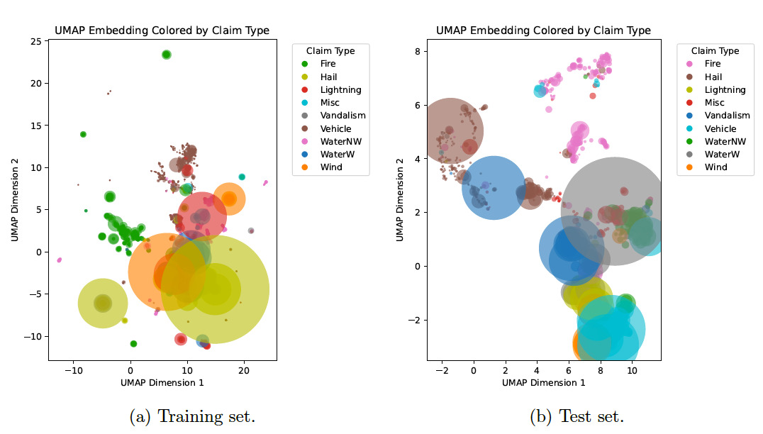
To dive a bit deeper into the semantic relationships captured within the claim descriptions, we first considered a conversion of claim descriptions to semantic embeddings via the all-mpnet-base-v2 model with the SentenceTransformer library. Next, we passed these embeddings into the 2d UMAP algorithm and constructed the scatter plot in Figure 3, with loss type represented by color and relative loss amount reflected by the size of the scatter plot point.

Figure 3.UMAP dimensions 1 and 2 of claim description embeddings.

The UMAP process constructs a graph in high-dimensional space, where each node is a claim. Next, nearby claims are connected based on distances in embedding space. It estimates the data’s underlying structure and optimizes a low-dimensional layout that preserves the local relationships from the original graph. This process is similar to the $t$-SNE ($t$-distributed stochastic neighbor embedding) algorithm but is faster and more faithful to global structure (McInnes et al. 2018).

As a result, the proximity of points within the UMAP visual implies semantic similarity. A number of clusters emerged, demonstrating that the embedding model successfully captured differences in language associated with specific event types. Some overlap is visible, which may indicate shared language within descriptions. Larger circles represent relatively high-loss events. Large losses appear in multiple clusters, suggesting that loss isn’t driven by description alone, and multiple claim types (e.g., fire, wind, etc.) can cause significant loss. However, a lack of large losses is evident in some clusters (e.g., hail, lightning).

4. Prompt engineering

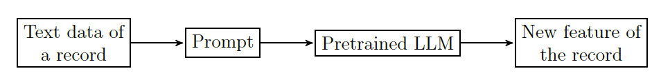
This section introduces prompt engineering, which plays an essential role when using pretrained LLMs to create features from text data. A prompt is an input provided to an LLM to produce the desired output. In other words, a prompt is a set of instructions an LLM uses to predict the desired results. Prompt engineering refers to the process of designing and refining input prompts to optimize the performance of LLMs such as ChatGPT.

Figure 4 shows a schematic diagram of how to use a pretrained LLM to create features from text data.

Figure 4.Schematic overview of using a pretrained LLM to generate new features.

4.1. Prompt-based learning

In traditional supervised learning systems for text data, we develop a model $P(\mathbf{y}\vert \mathbf{x}; \mathbf{θ})$ to predict an output $\mathbf{y}$ (e.g., a label) for an input $\mathbf{x}$. The model parameters $\mathbf{θ}$ are learned by using a dataset that contains pairs of inputs and outputs. The main issue with supervised learning is that labeled data are needed to train a model $P(\mathbf{y}\vert \mathbf{x}; \mathbf{θ})$. For many tasks, however, it is difficult to find large quantities of labeled data. Prompt-based learning circumvents this issue by using a pretrained LM that models the probability $P(\mathbf{x}; \mathbf{θ})$ of text $\mathbf{x}$ itself and using this probability to predict $\mathbf{y}$.

Prompt-based learning consists of three major steps (Liu et al. 2023): prompt addition, answer search, and answer mapping. In the first step, a prompting function $f_{p}(\mathbf{x})$ is used to convert an input text $\mathbf{x}$ into a prompt $\mathbf{x}'=f_{p}(\mathbf{x})$. In the majority of existing work, the prompt function is a template that includes two slots, an input slot and an answer slot. For example, the following template can be used as a prompt function for insurance text data:

$$\small{\begin{aligned} f_p(\mathbf{x}) ={}& \text{Incident description: } \mathbf{x}. \\ & \text{You are an assistant that classifies property} \\ & \text{insurance incidents by risk severity into} \\ & \text{one of three categories: 'low', 'med', or 'high'.} \\ & \text{Only return the classification.} \end{aligned}\tag{1}}$$

In the above prompt function, the first sentence is the input slot. The second and the third sentences form the answer slot.

In the second step, a pretrained LM is employed to search the highest-scoring text $\mathbf{z}$ based on filled prompts. For example, the filled prompt corresponding to the prompt given in Equation (1) can be:

$$\begin{aligned} f_{fill}(\mathbf{x},\mathbf{z}) = & \hbox{ Incident description: } \mathbf{x}. \\&\hbox{ Risk severity classification: }\mathbf{z}. \end{aligned}\tag{2}$$

The pretrained LM will search over the set of potential answers by calculating the probability of the filled prompts:

$$\hat{\mathbf{z}} = \arg\max_{\mathbf{z}\in \mathcal{Z}} P(f_{fill}(\mathbf{x}, \mathbf{z}); \mathbf{θ}),$$

where $\mathcal{Z}=\{\hbox{`low'}, \hbox{`med'}, \hbox{`high'}\}$.

In the third step, the highest-scoring answer $\hat{\mathbf{z}}$ is mapped to the highest-scoring output $\hat{\mathbf{y}}$. This step is usually trivial as the answer is the output required by the underlying task. In some situations, multiple answers will be mapped to the same output.

4.2. Principles of prompting

Because LLMs generate outputs based on the prompt they receive, the quality and structure of the prompt significantly influences the accuracy, relevance, and usefulness of the response. Phoenix and Taylor (2024) introduced five principles of prompting, which we briefly introduce in this subsection.

The first principle is to give clear direction. The prompt should be clear, unambiguous, and specific. Vague prompts tend to produce vague answers. Role-playing is a good way to create prompts. For example, in the prompt given in Equation (1), we give the LLM the role of the assistant who is tasked to classify property insurance incidents.

You are an assistant that classifies property insurance incidents by risk severity  into one of three categories: low, med, or high. Classify the following incident: lightning damage to tree, fire alarm panel.

You are an assistant that classifies property insurance incidents by risk severity  into one of three categories: low, med, or high. Classify the following incident: lightning damage to tree, fire alarm panel. Only return the classification name.

The second principle is to specify the output format. LLMs such as ChatGPT can produce output in different formats. For classification tasks, if we only need the classification categories, we need to specify this in the prompt. For instance, if we give the prompt shown in the first example to ChatGPT, we see the following output:

Classification: med

Reasoning:

Lightning damage to a tree typically represents a relatively low risk unless it results in secondary hazards (e.g., falling onto property or causing fire).

Damage to the fire alarm panel can have significant implications for fire safety and may require immediate repair or replacement to comply with safety codes.

The combination of electrical system impact and potential interruption to building safety mechanisms elevates the incident above low risk, but it does not involve structural damage, injury, or major fire, so it does not qualify as high risk.

If we use the prompt shown in the second example, the output produced by ChatGPT is “med.” By adding one additional instruction to the prompt, we got the classification category as the desired output.

The third principle is to provide examples. In the literature, a zero-shot prompt is where LLMs are asked to perform a task without giving any examples of how to do it. One-shot prompting provides one example, and few-shot prompting provides a few examples. Zero-shot prompting is useful when we want concise instructions or do not have labeled examples handy. It is especially effective with modern LLMs that have been trained on a wide variety of tasks.

The fourth principle is to evaluate the quality of the output generated by the language model. In many practical applications, this evaluation is performed informally through a process of trial and error—users iteratively modify prompts and assess the responses by manually inspecting their relevance, accuracy, or usefulness. While this approach can be effective, it is often inefficient and time-consuming, particularly when scaling up the use of LLMs.

A more systematic and scalable strategy is to incorporate a feedback or evaluation loop into the prompting workflow. This loop can include human-in-the-loop assessments, automated metrics, or comparison against ground truth data, depending on the task. Such a mechanism allows for more objective and consistent evaluation of outputs, enabling iterative refinement of prompts based on measured performance. However, it is important to consider the cost implications of this approach, especially when using commercial LLMs that charge per token. Each round of evaluation can incur significant expenses. Therefore, implementing an evaluation loop must strike a balance between improving prompt quality and managing computational and financial resources effectively.

The fifth principle is to divide the labor, which means breaking down a complex or large task into smaller, more manageable components. This modular approach not only simplifies the overall problem but also enables more focused and effective prompting for each subtask. By addressing one step at a time, users can design clearer prompts and achieve more reliable outputs from the language model.

4.3. Batch prompting

Batch prompting is the practice of sending multiple prompts at once to a language model in a single application programming interface (API) call or request. It is commonly used to process a set of similar tasks or inputs in parallel, rather than one at a time.

Batch prompting is beneficial in that it reduces overhead and latency by handling multiple prompts in one operation, and it is cost-effective. Many LLM APIs (such as OpenAI’s ChatGPT) allow batching, which can reduce per-prompt costs.

Batch prompting has two approaches. The first is to combine multiple prompts in a list and send the list to an LLM in a single API call. The LLM then will return a list of responses. The second is to combine multiple prompts into a single prompt.

The following are descriptions of 5 insurance incidents:
1. lightning damage
2. lightning damage at Comm. Center
3. lightning damage at water tower
4. lightning damage to radio tower 
5. vandalism damage at recycle center
You are an assistant assigned to classify the risk severity into one of three categories: low, med, or high. Return only the classification name for each of the incidents

For instance, if we give the prompt shown in the example above to ChatGPT, we see the following output:

1. med
2. med
3. high
4. high
5. med

This example shows that multiple incidents can be classified using a single prompt.

5. Empirical analysis

This section presents some empirical results of using LLMs to extract features from insurance text data. ChatGPT and Llama represent two leading LLMs. ChatGPT is a commercially available, highly polished model optimized for general-purpose use; it offers strong performance. In contrast, Llama is expected to continue the open-source tradition, enabling researchers and developers to download, fine-tune, and deploy models locally.

We used the ChatGPT-4o model (cutoff date October 2023) and the Llama-3.2-3B model (cutoff date December 2023) to classify incident severity into different categories based on incident descriptions.^[2] ChatGPT-4o is hosted in the cloud, fine-tuned for safety and alignment, and designed for seamless use in commercial applications. Llama-3.2-3B is a smaller 3-billion-parameter open-weight model from Meta, designed for lightweight local deployment and research. The classification labels generated by the LLMs were subsequently incorporated into a gamma GLM to evaluate their effectiveness in predictive modeling. Figure 5 presents a flowchart illustrating the overall data analysis process.

Figure 5.A flowchart of entire data analysis process.

5.1. Classification accuracy

We applied the two LLMs to classify the incident severity into two categories (low and high), three categories (low, medium, and high), and five categories (negligible, low, medium, high, and catastrophic). The cost of using ChatGPT-4o for these tasks was $26, and the runtime was about 2 hours.

Tables 4, 5, and 6 show the contingency tables of the results produced by ChatGPT-4o and Llama-3.2-3B. For the two-category results, categories NA, Low, and Hig denote unknown, low, and high, respectively. For the three-category results, categories NA, Low, Med, and Hig correspond to unknown, low, medium, and high, respectively. For the five-category results, categories NA, Neg, Low, Med, Hig, and Cat correspond to unknown, negligible, low, medium, high, and catastrophic, respectively. We assigned the output of an LLM to the category “unknown” when the model did not produce a valid classification. This occurred in cases where the text description of an incident was missing or contained no meaningful information, or when the LLM failed to generate a classification and returned an error.

Table 4 shows the contingency tables between the two-category result and the three-category result. Table 4(a) shows that when ChatGPT-4o was prompted to classify incidents into two categories, 2,892 ($1+1,042+1,849$) incidents were classified into the low category. When ChatGPT-4o was prompted to classify incidents into three categories, 3,637 ($1,849+1,788$) incidents were classified into the medium category. The low-category incidents from the two-category result were split into the low-category and the medium-category in the three-category result.

Comparing Tables 4(a) and 4(b) shows that ChatGPT-4o produced more consistent results than Llama-3.2-3B. For example, low-category incidents from the two-category result were not classified into the high-category from the three-category result by ChatGPT-4o. However, the two-category result and the three-category result produced by Llama-3.2-3B were mixed.

Figure 6.Box plots of log-loss by risk classes for the two-category approach produced by ChatGPT-4o and Llama-3.2-3B on the training set.

Figure 7.Box plots of log-loss by risk classes for the three-category approach produced by ChatGPT-4o and Llama-3.2-3B on the training set.

Figure 8.Box plots of log-loss by risk classes for the five-category approach produced by ChatGPT-4o and Llama-3.2-3B on the training set.

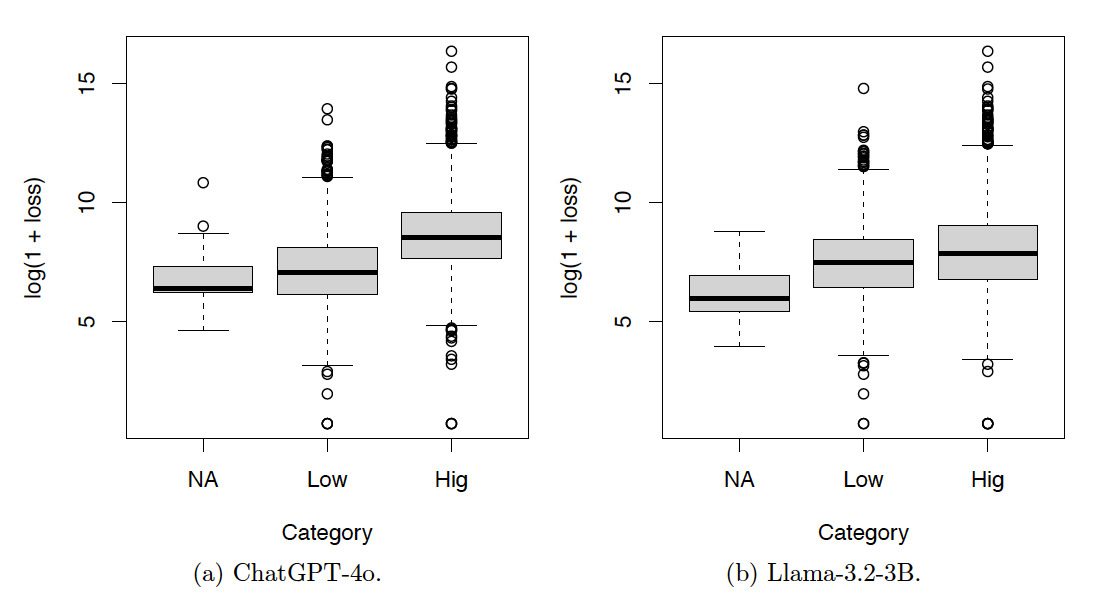
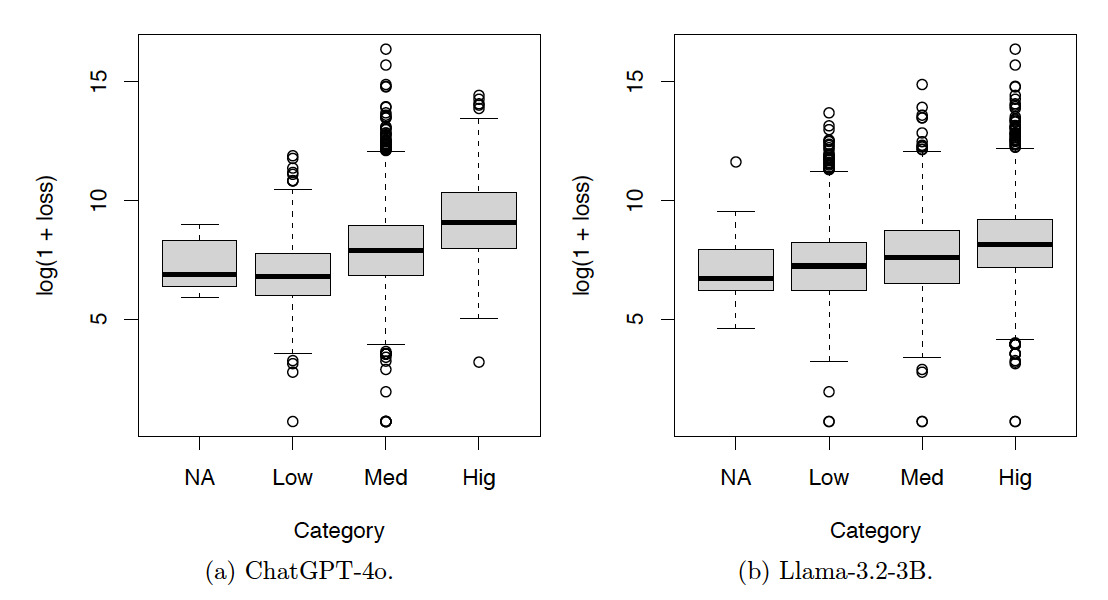
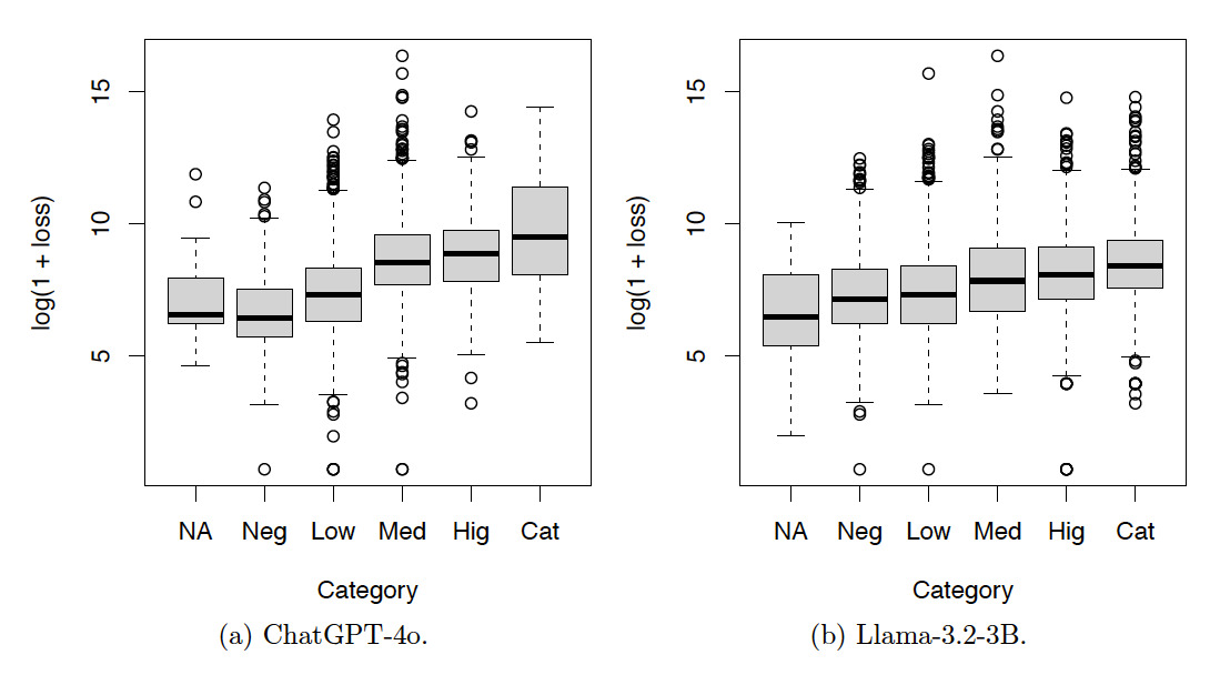
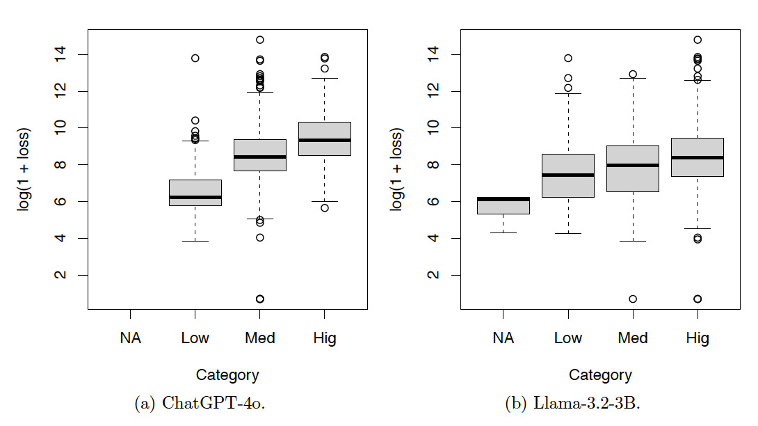
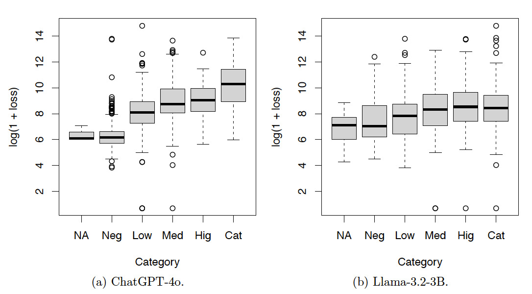
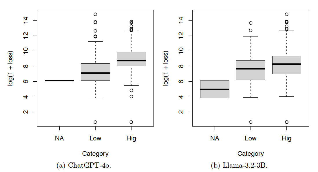
Figures 6, 7, and 8 show the box plots of the log-loss by risk categories for the training set. The risk categories were produced by ChatGPT-4o and Llama-3.2-3B based on the incident text descriptions in the training set. The category NA includes the incidents not classified by the LLMs. Categories Neg, Low, Med, Hig, and Cat denote incidents with severity levels from low to high. Summary statistics corresponding to these figures are also provided in Appendix A. Given the increasing patterns of the median log-loss in the box plots, the risk categories obtained by both LLMs make sense.

Figure 9.Box plots of log-loss by risk classes produced by ChatGPT-4o and Llama-3.2-3B on the test set.

Figure 10.Box plots of log-loss by risk classes produced by ChatGPT-4o and Llama-3.2-3B on the test set.

Figure 11.Box plots of log-loss by risk classes produced by ChatGPT-4o and Llama-3.2-3B on the test set.

Tables 7, 8, and 9 and Figures 9, 10, and 11 show the results for the test set. The resulting patterns are similar to those of the training set.

In summary, the contingency tables show that the results produced by ChatGPT-4o are more consistent than those produced by Llama-3.2-3B. The box plots show that the results produced by both ChatGPT-4o and Llama-3.2-3B are meaningful.

5.2. Loss prediction

This section presents the loss prediction results by incorporating the risk categories produced by LLMs. The summary statistics of the loss variable are shown in Table 2. The risk categories produced by LLMs are ordinal categorical variables. It is common to treat ordinal categorical variables as continuous variables in regression analysis.

Figure 12.Line plots of the mean log-loss against the risk levels.

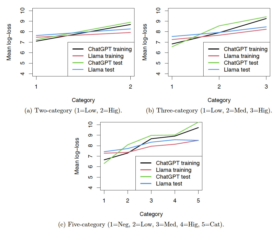
Figure 12 shows the line plots of the average log-loss against the risk levels, which are integers used to denote the risk categories. For the five-category risk classification, 1 to 5 denote the risk categories from negligible to catastrophic. The line plots show that the mean log-loss and the risk levels have approximately linear relationships. We can treat the ordinal risk categories obtained by LLMs as continuous variables in regression analysis.

We fitted gamma GLMs with the log link function to the training set. Then we used the fitted model to predict the log-loss for the test set. Table 10 shows the in-sample and out-of-sample validation measures of the fitted values from the gamma GLMs. The $R^2$ and $R_a^2$ were calculated as follows:

$$R^2 = 1 - \dfrac{\sum_{i=1}^n (y_i - \hat{y}_i)^2}{\sum_{i=1}^n (y_i - \bar{y})^2},\tag{3}$$

$$R_a^2 = 1 - \dfrac{(n-1)\sum_{i=1}^n (y_i - \hat{y}_i)^2}{(n-k-1)\sum_{i=1}^n (y_i - \bar{y})^2},\tag{4}$$

where $y_i$ and $\hat{y}_i$ denote the observed log-loss and predicted log-loss for the $i$th observation, $\bar{y}$ is the average observed log-loss, $n$ is the number of observations of the underlying dataset, and $k$ is the number of covariates, excluding the interceptor. The mean absolute error (MAE) was calculated as follows:

$$MAE = \sum_{i=1}^n \dfrac{\vert y_i-\hat{y}_i\vert }{n}.\tag{5}$$

The validation measures can be interpreted as follows. For $R^2$ and $R_a^2$, a higher value indicates a better fit. For MAE, a lower value indicates better predictive accuracy.

The validation measures in Table 10 show that including the labels obtained by LLMs produced a better fit. For example, the out-of-sample $R^2$ with the five-category label from ChatGPT-4o is 0.3971, which is higher than 0.3398 for the out-of-sample $R^2$ without any LLM labels. The $R_a^2$ and the MAE are consistent with this observation.

However, the $R^2$ values for the Llama-3.2-3B model are lower than those for the ChatGPT-4o model, indicating that ChatGPT-4o achieved better classification performance. This result is expected, given that ChatGPT-4o is believed to have over 1.8 trillion parameters, whereas Llama-3.2-3B has 3 billion. The significantly larger model size of ChatGPT-4o enables it to capture more complex patterns and relationships in the data, leading to more accurate predictions.

Table 11 shows the regression coefficients and their standard errors from the gamma GLMs fitted to the training set when the risk classification labels produced by ChatGPT-4o were used. Tables 11(b), 11(c), and 11(d) show that the labels produced by ChatGPT-4o are significant.

Table 12 shows the regression coefficients and their standard errors from the gamma GLMs fitted to the training set when the risk classification labels produced by Llama-3.2-3B were used. Tables 12(a), 12(b), and 12(c) show that the labels produced by Llama-3.2-3B are also significant.

We also compared our results with those obtained by Manski et al. (2021), who used correlation coefficients to measure the predictive performance. Table 13 reports the correlations between the observed log-loss and the log-loss predicted by different models for both the training and test sets. The baseline model without LLM-based labels achieved correlations of 0.6117 and 0.5956 on the training and test sets, respectively. Incorporating LLM-generated categorical labels improves these correlations, particularly for ChatGPT-4o, whose five-category labeling yields the highest out-of-sample correlation (0.6426). Results from Llama-3.2-3B show modest improvements over the baseline but remain slightly below ChatGPT-4o’s performance. Compared with the gamma double GLM from (Manski et al. 2021), which performs well on the training data (0.6638) but poorly on the test set (0.4868), the LLM-augmented models demonstrate better generalization and more consistent predictive power across datasets.

5.3. Reproducibility

Despite their strong performance, LLMs pose significant challenges for reproducibility. Unlike traditional statistical or machine-learning models, LLMs are typically proprietary and hosted through cloud-based APIs, meaning users cannot control or access the model weights or full training data. Consequently, model updates by providers can alter outputs even when identical prompts and parameters are used. Moreover, stochastic generation mechanisms, such as temperature sampling, introduce additional variability unless explicitly fixed. Differences in hardware, API versions, and tokenization can further affect results.

Table 14 shows the default values of the temperature parameter and the top-p parameter, which control the randomness of the LLMs’ outputs. Higher values for either parameter increase variability and creativity in responses. Lower values make the model’s outputs more deterministic and reproducible across runs. In all experiments described in this paper, the default values of the parameters were used as we did not specify any parameters for the LLMs.

To examine the variability of labels generated by LLMs, we ran the Llama-3.2-3B model four additional times. Table 15 presents the Chi-squared test statistics comparing pairs of label sets across the five runs, including the run discussed earlier. Since the critical value of the Chi-squared distribution with 25 degrees of freedom at the 1% significance level is 44.31, the results suggest that the labels generated across different runs of the LLM exhibit strong dependence.

Table 16 shows the validation measures of the gamma regression model using labels from five runs of the Llama-3.2-3B model. The table shows that the validation measures are consistent across runs, suggesting stable model performance.

5.4. Data exposure

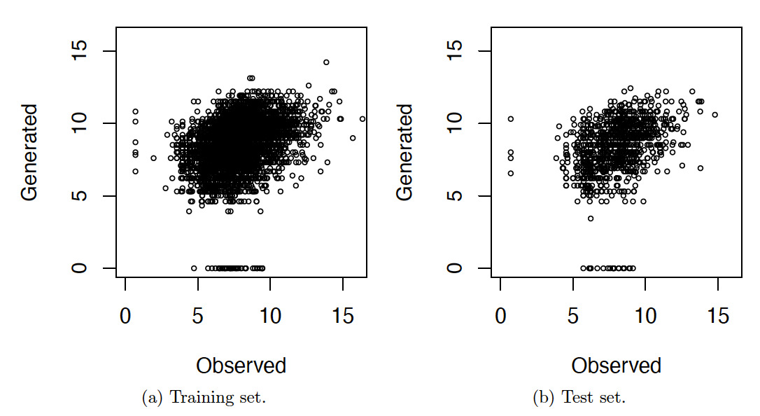
Pretrained LLMs are trained by using massive amounts of data from the internet. Because the dataset used in our study was obtained from the internet, it is likely that the data were used to train the LLMs. To examine whether the dataset was used to train the Llama-3.2-3B model, which is used in our study, we prompted Llama-3.2-3B to generate loss amount by proving the incident descriptions.

Figure 13.Scatter plots of the observed loss and the loss generated by Llama-3.2-3B in the log scale.

Figure 13 presents scatter plots of the observed loss amounts versus the loss amounts generated by Llama-3.2-3B, both in log scale. The plots show that the points are dispersed around the center, suggesting that the generated losses do not exhibit a systematic relationship with the observed losses and appear largely random.

6. Conclusions

This paper examined the use of LLMs to generate structured features from unstructured text data in the insurance setting, particularly with the purpose of improving loss prediction. We demonstrate that pretrained LLMs, specifically GPT-4o and Llama-3.2-3B, can effectively classify incident descriptions into ordinal severity categories via prompt-engineering techniques. These model-generated labels exhibit ordinal consistency, align with average loss magnitudes, and serve as informative predictors when incorporated into GLMs for severity estimation.

Empirical results indicate that the incorporation of LLM-derived features improves both in-sample and out-of-sample performance relative to models using only traditional variates. In particular, the five-category prediction yields the best accuracy, with higher $R^2$ and lower $MAE$ than baseline models.

These findings have important implications for actuarial science. First, they show that LLMs can serve as effective, low-cost tools for augmenting traditional actuarial models with context from unstructured text data. Second, the success of prompt-based approaches supports their applicability in settings where fine-tuning is infeasible. Finally, the interpretability of ordinal labels offers practical value for downstream modeling and decision makers.

Future work may investigate ensemble approaches, the integration of multiple LLMs, or hybrid models that combine LLM-generated features with traditional NLP techniques. Additionally, as open-weight models continue to evolve, evaluating their performance parity with proprietary models like GPT-4o remains an active area of interest. Overall, this research underscores the promise of LLMs in augmenting actuarial models and opens new directions for the use of text data in insurance analytics.

Acknowledgments

Guojun Gan and Christopher Shultz would like to acknowledge the financial support provided by the Casualty Actuarial Society (CAS). This research was supported in part through computational resources provided by the University of Connecticut, Storrs, CT.