1. Introduction

The National Council on Compensation Insurance (NCCI) uses the term excess ratios or excess loss factors (ELFs) to refer generally to ratios where the numerator is some measure of expected amount of losses in excess of a given limit, and the denominator is a corresponding measure related to expected unlimited losses.^[1] Periodically, NCCI reviews and updates the ELF methodology. The 2014 update made many improvements over the 2004 update, and these improvements are discussed in this paper.

Most private employers in the United States are required to provide workers compensation coverage to pay for lost wages and medical expenses arising from work injuries. Hazard groups, as described by Robertson (2009), are collections of workers compensation classifications that have relatively similar ELFs over a broad range of limits. NCCI produces and files ELFs by state and hazard group for various per-occurrence loss limitations; NCCI also publishes the data and calculations used to produce the ELFs.

1.1. Overview of ELF Framework

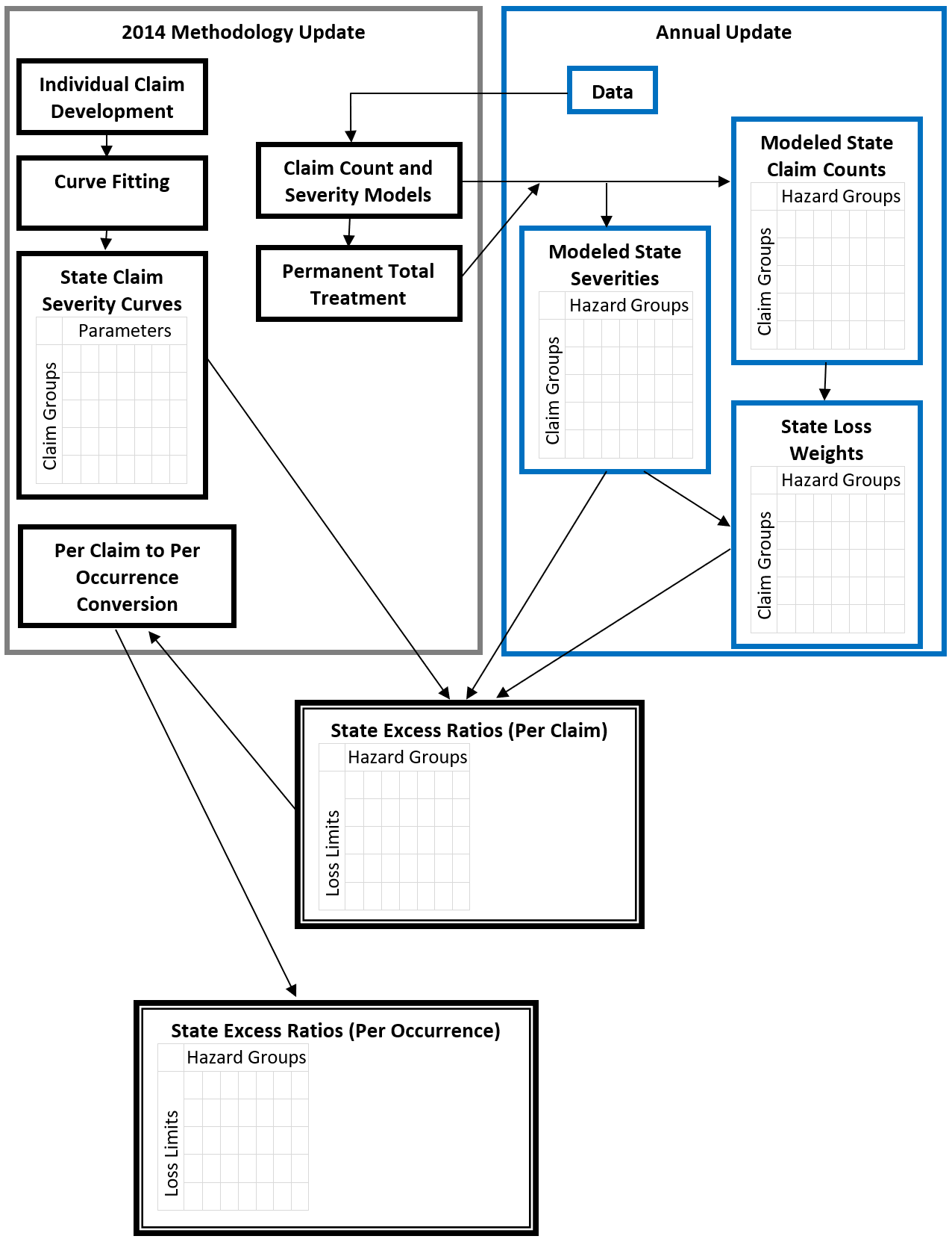
Gillam (1991) details NCCI’s general framework for computing excess ratios by hazard group and for individual states. The 2014 update makes changes to each component in the framework while retaining the general concepts. This section gives an overview of how those components fit together in the 2014 update while highlighting changes. Figure 1.1 provides a schematic representation of the components and relationships that are described in Section 1, as well as their relationships within the general framework of the annual update of ELF values..

Figure 1.1.Major components of the 2014 methodology and of the annual update of ELFs

For a given per-claim dollar limit, the per-claim excess ratio for each state–hazard group combination is a weighted average of excess ratios over five different claim groups. The claim groups used in the 2014 update are groupings based on reported injury types and other claim characteristics. Although these claim groups play role similar to the claim types in Gillam (1991), the injury types that form each grouping are different.

In the 2014 update, NCCI fits a severity distribution for each claim group and scales state–claim group excess ratios to reflect the average severity of claims for the claim group in that state and hazard group. The weights used for averaging the excess ratios across claim groups are the share of total losses in the state and hazard group for each claim group.

The excess ratios on a per-claim basis for each state–hazard group dollar limit are then converted to a per-occurrence basis and loaded with the appropriate expenses to calculate the desired type of ELF.

This paper discusses the following:

• Data used for the update

• Development of individual claims, and groups of claims, to ultimate

• Derivation of countrywide and state ELF curves by claim group

• Modeling of claim counts and average severities by state, hazard group, and claim group

• Derivation of state ELF curves including allocated loss adjustment expense (ALAE)

• Adjustment of per-claim ELFs to per-occurrence ELFs

• Implementation of the new methodology

1.2. Highlights of Changes from Previous Updates

Gillam and Couret (1997) and Corro and Engl (2006) have established the necessity of modeling ultimate losses that reflect loss development on an individual claim basis. They refer to this individual claim development as dispersion. To reflect dispersion, Gillam and Couret used different closed-form gamma-distributed divisors to model the development of open and closed claims separately; Corro and Engl replaced each open claim by 173 values reflecting developed loss amounts and adjusted for reopened claims. The 2014 update adds refinements to this idea, including reflecting differences in development by size of claim.

Another major theme is fitting distributions to each of the groupings of claims to the data. Gillam and Couret used, for each of their injury type groupings, maximum likelihood to fit the entire claim severity distribution. Corro and Engl used, for each injury type, the empirical distribution for the body of the distribution and fit a mixed exponential form to the tail, with parameters estimated by minimizing the sum of squared differences. The 2014 update, for each claim group, fits the body of the claim severity distribution to a mixed lognormal form. A Pareto form is fit to the tail, using extreme value theory (EVT) as described by McNeil (1997).

Finally, in terms of reflecting state differences in claim severity distributions for each state and groupings of claims, Gillam and Couret used one countrywide claim severity distribution for all states for each of their injury type groupings. Corro and Engl created state-specific claim severity distributions for each injury type by credibility-weighting the claim severity distributions calculated using state-specific claims experience with the countrywide claim severity distributions. The 2014 update reflects state differences via an adjustment related to the coefficient of variation (CV) of the state’s distribution for each claim group.

2. Organization of Data

2.1. Overview

The 2014 update uses unit data drawn from claim data on a case-incurred basis for 36 states reported under NCCI’s Statistical Plan for Workers Compensation and Employers Liability Insurance (“unit data”). Compared with the 2004 update, the 2014 update takes advantage of

• additional data elements, including the reported injured part of body and open/closed claim status; and

• claim data at maturities from 6th through 10th report (previously, only data through 5th report was available).

These changes reduce the uncertainty in several loss development analyses compared with previous updates. Specifically, Table 2.1 gives a summary of the data used for the major analyses in the 2014 update.

2.2. Claim Groups

In the 2014 update, NCCI categorizes each claim into one of the following five claim groups:

• Fatal

• Permanent total (PT)

• Likely to develop—permanent partial and temporary total (likely-to-develop)

• Not likely to develop—permanent partial and temporary total (not-likely-to-develop)

• Medical only

This assignment is based on the injury type^[2] and, for the likely-to-develop and not-likely-to-develop groups, certain other claim characteristics. These characteristics are based on NCCI’s class ratemaking injury type groupings as described by Daley (2012). They consist of the injured part of body and open/closed claim status reported in unit data at the claim’s first report and latest report.

The likely-to-develop claim group consists of the permanent-partial and temporary-total claims for which the injured part of body, together with the open/closed status, indicate a greater likelihood of upward development in the claim value over time. The not-likely-to-develop claim group consists of the remaining permanent-partial and temporary-total claims.

The use of the likely-to-develop and not-likely-to-develop groupings reduces the effect of claims moving between the permanent-partial and temporary-total injury types. This grouping helps improve the accuracy of loss development estimates. Claims in the likely-to-develop claim group tend to be more severe than those in the not-likely-to-develop claim group.

In contrast, NCCI’s 2004 update grouped claims by the injury types themselves:

• Fatal

• PT

• Permanent partial

• Temporary total

• Medical only

The use of claim groups in the 2014 update allows for changes in the distribution between them to be reflected automatically in the annual updates of ELFs.

3. Individual Claim Development

3.1. Overview: A Two-Step Approach

Where actuarial central estimates are of primary concern, it may suffice to determine the average development for a group of similar claims. However, the impact of development on individual claims is not uniform. Some open claims will have ultimate values much higher than originally estimated from applying a uniform development factor, and some lower. Gillam and Couret (1997) incorporated this phenomenon, which they referred to as dispersion. Mahler (1998) showed how Gillam and Couret’s work on dispersion fits into a more general mathematical framework.

Dispersion increases the variance of the severity distribution and produces higher ELFs than would otherwise result from applying a uniform development factor to all individual claims.

Additionally, past NCCI studies showed that individual claim development varies by size of claim, and specifically that smaller claims tend to have proportionally greater upward development than large claims (Evans 2011). The 2014 ELF update is the first to reflect this finding.

In the 2014 update, NCCI uses a two-step approach to reflect individual claim development. The first step reflects development and dispersion through 10th report. In this step, the average development applied to claims varies by size of claim, where the mean of the distribution of the development factor associated with a smaller open claim exceeds that of a larger open claim. We apply additional development and dispersion past 10th report in a second step that does not vary with the size of claim.

The 2014 use of claim information at 6th through 10th reports, not yet available during the 2004 update, incorporates data that goes further out to ultimate, thereby reducing the amount of extrapolation going into the final ELF. This change improves the estimate of dispersion and, in turn, the projection of individual claim development to ultimate.

3.2. Step 1: Size of Claim and Loss Development through 10th Report

NCCI divides the reported incurred value of each claim in a state, claim group, and report combination by the average claim size for the state, claim group, and report combination. The result is called an entry ratio because the mean across all claims in the cohort after this adjustment is 1. This normalization to entry ratios allows comparing claims across states and reports at a common basis, as well as pooling claims from different states and reports to create a countrywide pool of claims.

For each state–claim-group–report combination, NCCI constructs linear models that relate open claim loss development factors (LDFs) with claim size. These regression models have the logarithm of the LDF as the dependent variable and the log size of claim as the lone explanatory variable, as follows:

\[\begin{align} \ln\left( {LDF} \right) = &Intercept + Coefficient \\ &\cdot \ln\left( {Size\ of\ Claim\ in\ Entry\ Ratio} \right) + \epsilon \end{align}\]

A negative coefficient relates an increase in the size of claim with a decrease in the mean of the log LDF. As such, it relates changes in the size of claim to changes in the \(\mu\) parameter of the lognormal LDF distribution for the claim. Similarly, the standard error of the regression estimates the standard deviation of the error and is used to estimate the \(\sigma\) parameter. We apply this regression by size of claim through 10th report; beyond 10th report, we assume no relationship between size of claim and individual claim development.

In the above regression model for the left-side dependent variable \(\ln(LDF)\), we replaced the \(\ln\left( {Size\ of\ Claim\ in\ Entry\ Ratio} \right)\) term on the right-hand side with the following transformation:

\[f(x) = \left\{ \begin{matrix} x - 1,\ \ & x < 1 \\ \ln x,\ \ & x \geq 1 \\ \end{matrix} \right.\ \left\{ \begin{matrix} x - 1,\ & x < 1 \\ \ln x,\ & x \geq 1 \\ \end{matrix} \right.\]

This transformation was found to produce a reasonable value for the claim size entry ratio explanatory variable. A straight log transformation worked well for entry ratios above unity, but it produced aberrant behavior for small entry ratios near zero, where the log transformation approached negative infinity. To address this issue, we used the linear transformation for entry ratios below unity. More details on the parameters of the application of development by size of claim can be found in appendices B.1, B.2, and B.3.

3.3. Step 2: Loss Development and Dispersion beyond 10th Report

NCCI reflects dispersion beyond 10th report by treating each open claim at ultimate as a lognormal distribution. In contrast, each closed claim is treated as a point mass. Because claim information is not available past a 10th report in unit data, we determined claim closure rates past 10th report by selecting maximum additional durations of claims beyond 10th report by claim group. We also reviewed claims data from NCCI Financial Data Call 31 (Large Loss and Catastrophe) for information past a 10th report such as observed dispersion and claim closure.

More details on the parameters of the lognormal dispersion models can be found in appendices B.1, B.2, and B.4.

3.4. Final Adjustments to the Combined Development

To account for claims reopening, the closed claim share of total losses is adjusted downward, and the open claim share of total losses is adjusted correspondingly upward, with the adjustments varying by claim group.^[3]

As a final step, the total developed expected loss for open claims is balanced by state, report, and claim groups to an open-only LDF. We calculate this measure from the state’s LDFs for both open and closed claims underlying NCCI rate and loss cost filings. These LDFs are adjusted to an open-only basis, using the empirical percentage of losses for claims that are open by state, report, and claim group.

4. Curve Fitting

4.1. Overview

For each claim group, NCCI pools the developed and dispersed claims data for all 36 available states to determine a countrywide claim severity distribution. This claim severity distribution has a mixture of two lognormal distributions for the body and a generalized Pareto distribution for the tail. Parameters for the mixed lognormal distribution are determined by best fit to the data for regions where there was enough data to be credible. The point of transition between the main body and the Pareto tail is called the splice point. Parameters for the generalized Pareto distribution and the splice points are selected according to EVT, specifically by choosing Hill estimator parameters using peak-over-threshold (POT) charts for the right-hand tail region where data was sparse.

To produce the state-specific distributions for each claim group, NCCI adjusts the lognormal parameters of the countrywide distribution using a statistic for approximating the CV for each state relative to countrywide. We refer to this statistic as the R-value and use this R-value to adjust the parameters of the mixed lognormal curves; we do not adjust the tail of the Pareto distribution by state.

In contrast, the 2004 update represented the body of the distribution using empirical excess ratio tables with the tail represented by a mixed exponential distribution, each determined by state and injury type. The advantages of the 2014 changes include the following:

• The countrywide distribution is much more resistant to outliers.

• The body of the distribution has a more compact representation via a closed functional form.

• There is a simple adjustment of the countrywide distribution to a state distribution to reflect changes in the shape of the state distributions.

• The mixed lognormal distributions fit the body closely to the expected excess ratios resulting from developed and dispersed claim data.

• The generalized Pareto distribution fits the tail more closely.

4.2. Form of Body of Claim Severity Distribution

Excess ratios behave well with mixtures of distributions, in the sense that the excess ratio function for a mixture can be expressed as a weighted average of the excess ratio functions of the component distributions. Additionally, lognormal distributions are generally a reasonable choice to represent claim severity distributions and have closed-form expressions for excess ratios and related values that are reasonably easy to work with.

Since our dispersion method treats open claims at ultimate as a lognormal distribution and closed claims as point masses, the results of the dispersion calculation can be regarded as a mixture of the resulting lognormals and point masses. This method naturally leads to representing the body of the excess ratio curve by using a mixture of lognormal distributions. Analysis of goodness-of-fit and related metrics showed that a mixture of two lognormal distributions provided sufficient accuracy to represent the body of the curve.

A nonlinear model routine is used to fit the excess ratio of a mixture of lognormal distributions to 5,000 excess ratio values determined from the development and dispersion model. The routine first uses maximum likelihood to fit a single lognormal, then uses those parameters to select starting values for fitting a mixture of two lognormal distributions through an iterative process designed to minimize the sum of squared differences.

4.3. Form of Tail of Claim Severity Distribution

The tail of the curve is represented as a generalized Pareto distribution, based on the POT method from EVT as described by McNeil (1997). Pareto-tailed distributions are easy to work with when calculating the excess ratio.

More details on the tail selection can be found in appendices A.1 and A.2.

4.4. Splicing of Body and Tail of Countrywide Claim Severity Distribution

When combined with the splice point and shape parameter for the Pareto tail, the weights and parameters of the lognormal mixture provide a complete specification of the excess ratio curve as well as the corresponding claim severity distribution. This representation of the countrywide excess ratio curve for a claim group requires the following eight values:

• Two \(\mu\) parameters, one for each of the two lognormal distributions

• Two \(\sigma\) parameters, one for each of the two lognormal distributions

• One weight parameter for the mixture of the lognormal distributions

• One splice point parameter

• Two parameters for the generalized Pareto distribution

Formulas for the excess ratio for the lognormal and Pareto distributions provide closed-form expressions that are well-behaved and easy to work with for determining excess ratios and related values.

More details on the countrywide curves can be found in appendix C.1.

4.5. Relationship between Countrywide and State Distributions

For a distribution of a given form, the CV is among the most useful statistics for determining the shape of the distribution. The CV is especially useful when working with excess ratios because there is a closed-form expression relating the area under the excess ratio curve with the CV of the claim severity distribution. This relationship motivates using the CV to adjust the countrywide curves for each claim group to a state level. We considered three possibilities related to the CV: (1) the ordinary sample CV of untransformed losses, (2) the sample CV of the logarithm of the losses, and (3) the standard deviation of log losses. We chose to use the standard deviation of log losses because it produces the least bias and is most resistant to outliers. Additionally, our analysis suggested that it is appropriate to assign a credibility, based on the claim count volume, to the standard deviation of the log losses.

Note that the \(\sigma\) parameter of a lognormal claim severity distribution (the standard deviation of log losses) is related to the CV of the severity distribution:

\[CV^{2}\ + \ 1\ = \ e^{\sigma^{2}}\]

Each state–claim group combination is assigned a credibility based on claim count volume. The complement of credibility is the standard deviation of log losses for that claim group countrywide. We apply the resulting credibility-adjusted state R-value to the parameters of each of the countrywide mixture of lognormal distributions to determine state-specific excess ratio curves by state and claim group.

More details on adjusting the countrywide curves to a state level can be found in appendix C.2.

5. Estimation of State Severities and Loss Weights Using Bayesian Statistical Models

5.1. Overview

Once we have excess ratio curves by state and claim group that are normalized to a mean of 1 (as explained in Section 3.2), we then require two more sets of values to calculate the excess ratio at a given loss dollar limit in each state and hazard group. The first is the average cost per claim (called severity) for each claim group, and the second is the percentage of total loss dollars in each claim group (called loss weights).

The severity for each claim group is used to convert the loss limit from a dollar basis to an entry ratio basis. The excess ratio curve for the corresponding claim group is used to find the excess ratio for the claim group at the loss limit. These excess ratios by claim group are weighted together using state loss weights by claim group to obtain the desired by-state excess ratio for the given loss limit.

This method is the same general procedure described in Gillam (1991).

During the annual review, NCCI calculates updated severities and loss weights by state, hazard group, and claim group. These empirical values are based on five policy periods of unit data underlying the most recently approved rate or loss cost filings. In the 2014 update, NCCI enhanced the methodology to calculate these severities and loss weights, using multilevel and hierarchical statistical models to increase year-to-year stability while maintaining responsiveness to state and hazard group differences.

We use one Bayesian hierarchical model to estimate claim counts and another to estimate severities. We combine the results of the two models to produce loss weights.

We make an additional stabilizing adjustment due to the large year-to-year fluctuations inherent in the emergence of PT claims. Initial severities and claim counts for PTs are estimated via the same Bayesian hierarchical models as for the other claim groups. However, in annual updates of ELFs, the PT severity is trended forward, and the share of PT claim counts relative to all lost-time claim counts is kept constant. In this way, movement in the frequency of the PT claim group is stabilized, changing in proportion to the state’s lost-time claim frequency.

In contrast, in the 2004 update, the severities and loss weights were calculated based on developed, trended, and on-leveled data (the same data that are inputs to the Bayesian models). Because this method allowed for significant year-to-year fluctuations in the ELFs, the severities and loss weights were examined during the annual review for reasonableness and year-to-year fluctuations. Ad hoc adjustments were made as appropriate, usually to the PT severities and loss weights. The resulting ELFs calculated in one year were then averaged with the result of the ELFs calculated in previous years as an additional stabilizing adjustment.

Both the 2004 and 2014 updates use five policy periods of data to calculate severities and loss weights. However, due to the use of Bayesian models to estimate claim counts and severities, as well as the separate treatment of PTs, none of those ad hoc adjustments or weighted averages are still needed. The 2004 update stabilizing adjustments are not made to ELFs produced under the 2014 update.

5.2. Claim Count Model

The Bayesian hierarchical model to estimate claim counts specifies the following main effects and cross terms for claim frequencies for each state–policy-period–claim-group–hazard-group combination:

• Claim group differences

• State differences

• Policy period differences

• Hazard group differences within each claim group

• Interactions between state and claim group differences

• Interactions between state and hazard group differences

The model performs three major steps to get the expected claim count for each state–policy-period–claim-group–hazard-group combination:

1. For each state and hazard group, start with the known exposure (payroll) by policy period.

2. Adjust the exposure to a common time period by multiplying by the corresponding policy period factor.

3. Calculate an expected claim count for the given state–claim-group–hazard-group combination by multiplying together the main effects and cross terms.

Details about the model, including model specification and additional structure for the parameters, can be found in appendix D.1, with an illustration for a sample state shown in exhibit D.1.

5.3. Severity Model

The Bayesian hierarchical model to estimate severity is similar to the claim count model, specifying the following main effects and the cross term for claim severities for each state–claim-group–hazard-group combination:

• Base severity for claim group

• State differences

• Hazard group differences within each claim group

• Interactions between state and claim group differences

The model performs two major steps to get the expected severity for each state–claim-group–hazard-group combination:

1. For each claim group, calculate a base severity over all states and hazard groups.

2. Calculate the expected severity for the given state–claim-group–hazard-group combination by multiplying together the main effects and the cross term.

Details about the model, including model specification and additional structure for the parameters, can be found in appendix D.2, with an illustration for a sample state shown in exhibit D.2.

5.4. Treatment of PT Claims

PT claims contribute to a significant portion of the ELFs, particularly at higher loss limits. PT claims also account for a comparatively small claim volume by state and hazard group and show high variability in loss amounts. These issues can combine to produce large year-to-year fluctuations in PT severities and loss weights, which, in turn, can result in large year-to-year fluctuations in the ELFs. In the past, NCCI averaged each year’s indicated ELFs with the ELFs of prior years and examined the severities and loss weights for all states, hazard groups, and injury types. Judgment was required where fluctuations in severities and loss weights led to large fluctuations in ELFs.

In the 2014 update, we increase the stability of severities and loss weights via the new Bayesian models. We calculate the claim counts and severities for PT claims separately from the other claim groups. For PTs, instead of the years of data used in the severity and claim count models for non-PT claim groups, we use the five years of data used to fit the excess ratio curves.

We generate the PT severities and claim counts based on two initial fixed values for each state and hazard group:

1. initial PT severity

2. initial ratio of PT claim counts to non-PT lost-time claim counts

To obtain the PT expected severity, we apply a two-stage trend to the initial PT severity.

In the 2014 update, the first stage initially used annual trend factors of 5.0% for indemnity and 6.7% for medical. These trend factors were the average annual changes from accident years 2002 to 2008 from NCCI’s 2012 Countrywide Frequency and Severity Analysis. The period 2002 to 2008 was selected to avoid different frequency trends that occurred for different claim sizes before 2002 and the effects of the Great Recession on severities after 2008.

However, the observed indemnity and medical trends in subsequent years have decreased since the original choice of trend factors. For the annual review filed in 2016, NCCI has started to use a different first-stage trend, which is now a blend of six years. The original 5.0% indemnity and 6.7% medical trend are blended with newly selected trends of 2.0% indemnity and 3.0% medical. The newly selected trends will receive an additional year’s worth of weight in each subsequent annual review.

The second stage uses separate state-specific trend factors for indemnity and medical, from the most recent state loss cost or rate filing.

To update the PT expected claim count each year, we multiply the sum of the claim counts for the fatal, likely-to-develop, and not-likely-to-develop claim groups by the initial ratio of PT claim counts to non-PT lost-time claim counts. This procedure assumes that the ratio of PT claims to non-PT lost-time claims stays constant over time.

To obtain the PT loss weight, we combine the PT severities and claim counts.

Exhibits E.1 and E.2 in appendix E provide illustrations for a sample state.

6. Treatment of Losses including ALAE

6.1. Overview

In the 2004 update, the same excess ratio curves were used for loss excluding ALAE and loss including ALAE. To reflect the inclusion of ALAE, an ALAE factor was applied to only the most severe injury types (fatal, PT, and permanent partial) when calculating severities on a basis including ALAE.

This method changed with the 2014 update. NCCI reviewed paid ALAE in unit data and found that ALAE relative to loss is a smaller proportion of dollars for larger claims in the more “severe” claim groups. We reflect this difference by generating separate excess ratio curves on a loss-including-ALAE basis. We also apply ALAE factors that vary by claim groups when calculating severities that include ALAE. These procedures generate a separate set of excess ratio curves shaped differently than the loss-only curves for the same claim group.

6.2. Excess Ratio Curves including ALAE

In the 2014 update, NCCI generates countrywide excess ratio curves on a loss-including-ALAE basis. This is done by first adding an ALAE amount to each claim. For closed claims, we use the reported paid ALAE. For open claims, we analyze development patterns in the ratio of paid ALAE to paid loss by claim group and size of claim. Based on that analysis, we adjust the paid ALAE to reflect differences by size of claim and claim group. For each open claim, we adjust the paid ALAE by multiplying it by a development factor that differs by claim group and claim size ranges. As a final step, we balance the total ALAE dollars to a target ALAE percentage by state and period.

Then, for each claim group, we develope, disperse, and fit to curves the individual expected excess loss and ALAE claim amounts, following the same procedure described previously for losses not including ALAE. The same generalized Pareto tail distributions by claim group are spliced to the tail, as was done for losses not including ALAE. State curves are generated by adjusting these countrywide curves including ALAE using the R-value calculated from losses including ALAE, as was done for losses not including ALAE.

Consistent with the determination of excess ratios for losses without ALAE, the final state curves are generated by weighting those state curves with excess ratio curves of losses not including ALAE. These weights reflect the ratio of the state ALAE factor (updated during each state’s annual review) to the overall countrywide ALAE factor of 1.127, which was used in the original fitting of the countrywide excess ratio curves on a loss-including-ALAE basis.

For a given dollar loss limit, the excess ratio for losses including ALAE can be greater than or less than the excess ratio for losses not including ALAE. For a given dollar limit, even when the excess ratio for losses including ALAE is less than the excess ratio for losses not including ALAE, the excess dollar amount of losses including ALAE is at least as great as the excess dollar amount of losses not including ALAE. Including ALAE cannot reduce the dollars in excess of any limit.

A further refinement is done to excess ratios including ALAE for consistency with those not including ALAE. Upper and lower bounds related to the excess ratios not including ALAE are applied to excess ratios including ALAE. The upper bound represents the case where the additional ALAE has full contribution to the excess on an including-ALAE basis (i.e., an additional dollar of ALAE contributes to the excess including ALAE by one dollar); the lower bound represents the case where additional ALAE has no contribution to the excess on an including-ALAE basis (i.e., an additional dollar of ALAE does not contribute to the excess including ALAE).

The parameters for the excess ratio curves on a loss-including-ALAE basis are fixed (as are curves for loss excluding ALAE). However, these adjustments for the state ALAE factor, which may change during the annual review, as well as the upper and lower bounds, contribute to annual changes in ELFs for losses including ALAE.

More details on the specific excess ratio formulas for losses including ALAE can be found in appendix F.

6.3. Severities including ALAE

In the 2014 update, NCCI estimates countrywide ALAE percentages by claim group. These percentages are converted to relativities to a total countrywide ALAE percentage. Then, in the annual review, the percentages are applied to an overall state ALAE percentage, yielding state ALAE percentages by claim group. We then apply the state ALAE percentages by claim group to pure loss severities to obtain severities including ALAE. Table 6.1 shows the countrywide ALAE percentages by claim group. Exhibit G.1 in appendix G provides an illustration for a sample state.

This change represents another refinement to the methodology. In the 2004 update, an ALAE factor was calculated for the fatal, PT, and permanent-partial injury types so that the ALAE dollars assigned to those injury types balanced to the state total ALAE dollars. The temporary-total and medical-only injury types were not allocated any ALAE dollars. Note the use of injury types as opposed to claim groups when adjusting severities to include ALAE. The 2004 algorithm resulted in a higher ALAE percentage for more serious injury types, especially for fatal and PT, and this result was not supported by subsequent empirical investigation.

7. Per-Claim to Per-Occurrence Adjustment

7.1. Overview

Occurrences are claims from the same policy that arise from a single event. In the context of ELFs in general, dollar limits can apply either on a per-occurrence basis or on a per-claim basis. The countrywide excess ratio curve is based on a model of per-claim excess ratios at ultimate, while filed state ELF values are based on per-occurrence excess ratios at ultimate. Therefore, we need a method to convert excess ratios from a per-claim basis to a per-occurrence basis.

For converting per-claim excess ratios to per-occurrence excess ratios, NCCI constructed a table for use in all states that relates per-claim and per-occurrence excess ratios. We compare claim characteristics between claims that were reported as part of a multiclaim occurrence to those that were not. We also estimate the probability of a claim belonging to a multiclaim occurrence. That estimate is based on a comparison of the likelihood of injuries on the same policy having the same date of injury with what was observed in the actual data.

In contrast, in the 2004 update, a collective risk model approach was used, which produced much smaller differences between per-occurrence and per-claim excess ratios.

7.2. Claims from Multiclaim Occurrences vs. Single-Claim Occurrences

In the 2014 update, we considered using a collective risk model to aggregate individual claims into occurrences, as was done in the 2004 update. We rejected that approach because we observed positive correlation in claim size between claims within an occurrence (correlation coefficient of about 0.25), which violates the independence assumptions of the collective risk model.

Instead, we categorize occurrences as singletons and multiples, depending upon whether more than one claim arose from the occurrence. The catastrophe code that is reported in unit data identifies whether an individual claim on a given policy belongs to a multiclaim occurrence. For our purposes, the quality of catastrophe code data is suitable for identifying a subset of multiples but not the entire subset. We assume that this subset of multiples identified from reported data is representative of all true multiples, and we look at claim characteristics of this subset to draw conclusions about all multiples.

Such conclusions include the proportion of occurrences with exactly two claims, three claims, etc., as well as differences in claim characteristics between singletons and multiples. For example, claims within multi-claim occurrences, compared to singleton claims, have a higher mean severity, have a higher proportion of fatalities, and are more likely to be caused by an auto accident. Additionally, we found claim size of claims within a multiclaim occurrence to have a positive correlation of 0.25 with each other.

More details on the claim characteristics for multiples can be found in appendix H.

7.3. Probability of a Claim Belonging to a Multiclaim Occurrence

Because the subset of identified multiples does not include all multiples, we use an indirect simulation approach to measure the proportion of all claims that belong to a multiple occurrence. We look at claims data for the years 2000 to 2009 but exclude claims in which injuries were reported to occur on a Monday or on the weekend. This exclusion avoids effects from possible clustering of claims reporting on Mondays for claims occurring on the weekend. For each claim, we calculate the number of days from policy effective date to the date of injury, excluding weekends and Mondays, and call this figure the time index. For any pair of distinct claims, we consider two events:

    A. They are from the same policy.

    B. They have the same time index.

If there were no multiple occurrences, then these events should be independent of one another. The data reveals a positive correlation. We use a simulation routine that grouped claims on the same policy into occurrences. The simulation is run, varying the assumed probability that a claim is the first claim within an occurrence. As that probability increases, so does the correlation between events A and B. The runs for which the correlation is closest to the observed correlation indicates that about 2% of claims belongs in a multiple occurrence and that the average number of claims in a multiple occurrence is 2.71.

We use this procedure to express the countrywide excess ratio curve on a per-occurrence basis in terms of two excess ratio curves, both on a per-claim basis—one curve that reflects the frequency and severity by claim group for claims from singleton occurrences and another curve that reflects the characteristics of claims from multiple occurrences.

More details on the comparison of singleton- and multiple-occurrence claims and the excess ratio formulas can be found in appendix H. An illustration of per-occurrence excess ratios can be found in appendix I.

8. Implementation

The updated ELF values^[4] and the underlying methodology were filed in NCCI Item Filing R-1408 on June 16, 2014, and have been approved since December 3, 2014,^[5] for effective dates in 2014 to 2015.

ELF values are also used in NCCI ratemaking; the results of the updated values and methodology were incorporated into the loss cost and rate filings with effective dates in 2015 to 2016.

Additionally, as the 2014 ELF update provides methodology to determine the claim severity distribution, results from the update are being used in the update to the NCCI table of insurance charges (“Table M”) currently in progress.

8.1. Impact

The impacts of implementing the 2014 update’s methodology vary by state, occurrence limit, and hazard group. Because the state excess ratio curves in the 2014 update are obtained by adjusting the countrywide excess ratio curves, there are some patterns that generally hold across states. NCCI compared the ELFs calculated in the previous methodology with those calculated with the methodology in the 2014 update and found the following:

• At loss limits below $3 million, most excess ratios from the 2014 update are higher than in the previous update.

• At loss limits above $3 million, the excess ratios from the 2014 update are increasingly lower than in the previous update.

9. Conclusion

The 2014 update makes significant theoretical and practical improvements in the methodology while keeping much of the existing framework and fundamental ideas. The improvements result in a more accurate treatment of losses including ALAE, tails of the claim severity distributions that are more accurate with additional theoretical grounding, and increased year-to-year stability in the ELFs.

Acknowledgments

Many staff at NCCI contributed to the 2014 ELF update, including John Robertson, Jon Evans, Chris Laws, and Casey Tozzi. We also thank the NCCI Individual Risk Rating Working Group for their discussion and input.

Appendices

Appendix A.1. Mathematics of Excess Ratios

Given a claim severity distribution with the cumulative distribution function (CDF) \(F(x)\), we define the following standard terms:

• mean \(\equiv \mu_{F} = \int_{0}^{\infty}{{xf}(x){dx}}\)

• variance \(\equiv \ \sigma_{F}^{2} = \int_{0}^{\infty}{\left( x - \mu_{F} \right)^{2}f(x){dx}}\)

• standard deviation \(\equiv \sigma_{F} = \sqrt{\sigma_{F}^{2}}\)

• survival function \(\equiv S_{F}(x) = 1 - F(x) = \ \int_{x}^{\infty}{f(y){dy}}\)

• excess ratio function \(\equiv R_{F}(x)\)\(=\frac{\int_{x}^{\infty}{(y - x)f(y){dy}}}{\int_{0}^{\infty}{{yf}(y){dy}}}\)\(=\frac{\int_{x}^{\infty}{S_{F}(y){dy}}}{\mu_{F}}\)

• mean residual lifetime \(\equiv {MRL}_{F}(x)\)\(=\frac{\int_{x}^{\infty}{(y - x)f(y){dy}}}{\int_{x}^{\infty}{f(y){dy}}}\)\(= \ \frac{\mu_{F}R_{F}(x)}{S_{F}(x)}\).

When \(\mu_{F} = 1\), we have the equation:

\[\begin{align} \int_{0}^{\infty}{R_{F}(x)dx = \ \frac{\left( 1 + {{CV}_{F}}^{2} \right)}{2}}\text{ where }\\ CV_{F} =\text{ Coefficient of Variation}\ = \frac{\sigma_{F}}{\mu_{F}}. \end{align}\]

We use EVT to select a generalized Pareto distribution tail (select the splice point \(a\) and parameters \(m\) and \(b\)—see the following section) that applies to all states. This procedure was done for each claim group via the following steps:

• Normalize data to entry ratios; pool states and years.

• Plot the mean residual lifetime of losses and log of losses to create POT charts (see Embrechts, Klüpperberg, and Mikosch 2003, 352-370).

• Use POT chart of log-losses to determine the slope parameter \(m\) (Hill estimator) and the splice point \(a\) (see Embrechts, Klüpperberg, and Mikosch 2003, 330-335).

Appendix A.2. Useful Formulas

Lognormal

In what follows, \(\Phi(z) = \frac{1}{\sqrt{2\pi}}\int_{- \infty}^{z}e^{- \frac{t^{2}}{2}}{dt}\) denotes the CDF of the standard normal distribution. Therefore, the CDF of the lognormal distribution with parameters \(\mu\) and \(\sigma\) is given by:

\[F(r) = \Phi(z)\text{ where }z = \frac{lnr - \mu}{\sigma}\]

its mean by:

\[\overline{r} = e^{\mu + \frac{\sigma^{2}}{2}}\]

and its excess ratio function by:

\[R_{F}(r) = 1 - \Phi(z - \sigma) - r\frac{1 - F(r)}{\overline{r}}\ \]

and its MRL function by:

\[{MRL}_{F}(r) = \frac{\overline{r}\left( 1 - \Phi(z - \sigma) \right)}{1 - \Phi(z)} - r{\ .}\]

Generalized Pareto Distribution (GPD)

For the parameterization used here, which is not standard,^[6] the CDF of the GPD is given by:

\[G(b,m;x) = \left\{ \begin{matrix} 1 - \left( \frac{b}{mx + b} \right)^{\frac{m + 1}{m}} & m \neq 0 \\ 1 - e^{- \frac{x}{b}} & m = 0. \\ \end{matrix} \right.\]

Its mean is just the \(b\) parameter. Its excess ratio function is:

\[R_{G}(x) = \left\{ \begin{matrix} \left( \frac{b}{mx + b} \right)^{\frac{1}{m}} & m \neq 0 \\ e^{- \frac{x}{b}} & m = 0 \\ \end{matrix} \right.\ \]

and its mean residual lifetime function is linear:

\[{MRL}_{G}(x) = mx + b.\]

The case \(m > 0\) is the usual Pareto distribution.

Splicing

Fix a splice point a, and suppose we have a claim severity distribution with CDF F that we want to modify to a new distribution with CDF \(\widetilde{F}\) so that for losses greater than a, the new distribution \(\widetilde{F}\) follows a second distribution with CDF \(G\). The case of interest is when \(F\) is a mixture of lognormal distributions and \(G\) is a GPD. It is natural to specify this “spliced distribution” in terms of its survival function:

\[S_{\widetilde{F}}(x) = \left\{ \begin{matrix} S_{F}(x) & x \leq a \\ S_{F}(a)S_{G}(x - a) & x \geq a. \\ \end{matrix} \right.\]

Now suppose we have the equation:

\[{MRL}_{F}(a) = \mu_{G}.\]

Then \(\mu_{\widetilde{F}} = \mu_{F}\), and one can readily determine the excess ratio function of the spliced distribution \(\widetilde{F}\) from those of \(F\) and \(G\):

\[R_{\widetilde{F}}(x) = \left\{ \begin{matrix} R_{F}(x) & x \leq a \\ R_{F}(a)R_{G}(x - a) & x \geq a. \\ \end{matrix} \right.\ \]

When \(G\) is GPD with parameters \(m\) and \(b = {MRL}_{F}(a)\) we have:

\[R_{\widetilde{F}}(x) = \left\{ \begin{matrix} R_{F}(x) & x \leq a \\ R_{F}(a)\left( \frac{b}{m(x - a) + b} \right)^{\frac{1}{m}} & x \geq a. \\ \end{matrix} \right.\]

Appendix B.1. Parameters of the Lognormal LDF Dispersion Models: Overview

The kernel density distribution that the individual claim development and dispersion (D&D) model initially assigns to the open claim of size \(x\) (reopened claims are treated the same as open) and report \(t\) is a lognormal distribution with standard parameters:

\[\ln(x) + \mu(t;x)\text{ and }\sigma^{2}(t)\]

• Ratemaking LDFs by state, claim grouping, and report are converted to “open-only” LDF factors

• Those open-only factors are used to modify the first parameter by an additive constant by state, claim grouping, and report (flat factor in entry ratio space)

• That adjustment assures that the model has the same expected loss at ultimate as implied by the ratemaking LDFs, by state, claim grouping, and report

Appendix B.2. Parameters of the Lognormal LDF Dispersion Models: Details

As noted in Section 3, the D&D model adjusts open claims to an ultimate basis in two steps—first to a 10th report and then from a 10th report to ultimate:

• Step 1 (through 10th report)—D&D varies by size of claim based on regression

  • Linear regression considers individual claim development from report \(t\) to report 10 and relates it with the claim amount at report \(t\)

  • A linear regression model is determined using open claims for each of the 20 report-claim grouping combinations as follows:

    • four reports \(t\), for \(t = 6,7,8,9;\) and

    • five claim groupings

• Step 2 (beyond 10th report)—D&D does not vary by size of claim^[7]

  • Consider the pattern of variability of observed logarithms of annual LDFs from reports \(t\) to \(t + 1\), for \(t = \ 4,\ 5,\ 6,\ 7,\ 8,\ 9\)

  • Use exponential regression, tempered with judgment, and project those patterns from report \(t > 9\) to claim closure

The D&D steps 1 and 2 are not correlated. Sizes of loss and per-claim development beyond 10th report are not related.

Appendix B.3. Parameters of the Lognormal LDF Dispersion Models: Step 1 Further Details

For claims open at report t and within a claim grouping, a linear regression estimates the log per-claim LDF as a function of a transformed per-claim loss amount at report t.

• The regression equation is used to estimate the mean \(\mu_{1}(t;x)\) of the \(t\)th to 10th log LDF; this estimate varies with the size of claim \(x\).

  • Transforming the size of claim metric improves the fit, especially for the largest claims.

  • In place of entry ratio \(x\) as explanatory variable, the revised model uses a compressed size of claim metric \(\gamma(x)\):

\[\gamma(x) = \ln x\text{ for }x \geq 1;\ \gamma(x) = \ x - 1\text{ for }x \leq 1.\]

• The variance of the distribution of the residual gives an estimate of the variance \(\sigma_{1}^{2}(t)\) of the \(t\)th to 10th log LDF; this estimate does not vary with the size of claim \(x\).

• The proportion \(\rho(t)\) of claims open at report \(t\) that remain open at 10th is calculated from the claim data used in the regression.

Appendix B.4. Parameters of the Lognormal LDF Dispersion Models: Step 2 Further Details

The model assumes that beyond 10th report,

• the mean of the distribution of log annual LDFs is 0 for all claims and all years and

• the annual claim closure rate is constant for each claim grouping.

The variance \(\sigma_{2}^{2}\) of the second step is estimated for each claim grouping using

• a constant annual claim closure rate,

• projected variances of the distributions of annual log per-claim LDFs,

• exponential decay model as appropriate (becoming linear with a log vertical scale),

• a judgmentally assigned asymptote as the long-term estimate of the variance of the log annual LDF, and

• formulas for the decay model.

Let \(y(t) =\) empirical variance of annual per-claim LDF from report \(t\) to \(t + 1\). The formula to project variance is

\[y(t) = a + c \cdot e^{{bt}}\]

in which \(a\) is an assumed asymptotic long-term variance^[8] and \(b\) and \(c\) are constants to be estimated. The linear regression model with coefficient vector \(= \beta\),

\[\ln\left( y(t) - a \right) = \ln c + bt = \beta_{0}\ + \beta_{1}t + \epsilon(t),\]

is used to yield the estimates \(c = e^{\beta_{0}}\) and \(b = \beta_{1}\). The formula for the variance of 10th-ultimate log LDF is as follows, letting \(1–s\) be the constant annual claim closure rate and \(N\) be the maximum duration to closure after report \(t = 10\):

\[\begin{align} \sigma_{2}^{2} \approx &\left( \frac{a}{1 - s} \right)\left( 1 - \frac{Ns^{N}(1 - s)}{1 - s^{N}} \right) \\ &+ \left( \frac{ce^{10b}}{1 - e^{b}} \right)\left( 1 - \left( \frac{e^{b}(1 - s)}{1 - s^{N}} \right)\left( \frac{1 - \left( se^{b} \right)^{N}}{1 - se^{b}} \right) \right). \end{align}\]

The maximum additional duration to closure \((N)\) after 10 years by claim group is given in Table B.1.

In summary, to each open claim of size \(x\) at latest report \(t\), the D&D model assigns a mean \(\mu(t;x)\) and variance \(\sigma^{2}(t)\) to the log per-claim LDF distribution; with just two uncorrelated component steps:

\[\mu(t;x)\ = \ \mu_{1}(t;x)\ \text{and}\ \sigma^{2}(t)\ = \ \sigma_{1}^{2}(t)\ + \rho(t)\sigma_{2}^{2}\]

where:

• \(\mu_{1}(t;x) =\) linear estimate for the mean of the \(t\)th to 10th log LDF

• \(\sigma_{1}^{2}(t) =\) estimated variance of the \(t\)th to 10th log LDF

• \(\rho(t) =\) proportion of claims still open at 10th report

• \(\sigma_{2}^{2} =\) estimated variance of the 10th to ultimate log LDF.

The values \(\mu(t;x)\) and \(\sigma_{2}(t)\) are the standard parameters for the lognormal density model for the LDFs of an open claim of size \(x\) at latest report \(t\) (prior to balancing with ratemaking LDFs by state, claim group, and report).

Appendix C.1. Parameters of Countrywide Excess Ratio Curve as a Lognormal Mixture and Pareto Tail

This section describes the ingredients that go into the parametric form for expressing the excess ratio \(R(r)\) as a function of entry ratio \(r\). The severity distribution is a mixture of two lognormal distributions with parameters \(\mu_{1},\mu_{2}\) and \(\sigma_{1},\ \sigma_{2}\), respectively.^[9] The weight assigned the first component is denoted \(\omega_{1}\) and the weight assigned the second component is denoted \(\omega_{2} = (1 - \ \omega_{1})\). A Pareto tail distribution is spliced onto the lognormal mixture at an entry ratio denoted by \(a\) and termed the splice point (the splicing preserves an entry ratio mean of 1). The parameters used for the Pareto distribution are denoted \(b\) and \(m\), chosen to exploit the characterization of the Pareto distribution as one having a linear mean residual lifetime function of slope \(m\) and intercept \(b\), which is also the mean of the distribution.

The CDF of the lognormal components are:

\[F_{i}(r) = \Phi(z_{i})\text{ where }{\ z}_{i} = \frac{\ln r - \mu_{i}}{\sigma_{i}},\text{ where }i = 1,\ 2.\]

Their means are:

\[\overline{r_{i}} = e^{\mu_{i} + \frac{{\sigma_{i}}^{2}}{2}}\]

and in particular:

\[1 = \omega_{1}\overline{r_{i}} + \left( 1 - \omega_{1} \right)\overline{r_{2}}\]

as we are working with entry ratios. The excess ratio functions of the lognormal components are:

\[R_{i}(r) = 1 - \Phi\left( z_{i} - \sigma_{i} \right) - r\frac{1 - F_{i}(r)}{\overline{r_{i}}}{\ .}\]

The CDF of the lognormal mixture portion is:

\[F(r) = \omega_{1}F_{1}(r) + \left( 1 - \omega_{1} \right)F_{2}(r),\ r \leq a\]

and the excess ratio function for the lognormal mixture portion is loss-weighted average:

\[R(r) = \omega_{1}\overline{r_{1}}R_{1}(r) + \left( 1 - \omega_{1}\overline{r_{1}} \right)R_{2}(r),\ r \leq a.\]

The probability of surviving to the splice point is:

\[S = 1 - F(a)\]

and since the mean residual lifetime at the splice point must preserve a mean of 1, we have the following equation that can be used to find the value \(b\) to assign to the b parameter:

\[R(a) = bS.\]

The CDF of the Pareto tail portion is:

\[F(r) = 1 - S\left( \frac{b}{m(r - a) + b} \right)^{\frac{m + 1}{m}},r \geq a.\]

Finally, from the formula for the excess ratio of a Pareto distribution, we have the formula for the Pareto tail portion as:

\[R(r) = S\left( \frac{b}{m(r - a) + b} \right)^{\frac{1}{m}},r \geq a.\]

Appendix C.2. Deriving the State Excess Ratio Curves from the Countrywide Curves

The process starts with a credibility-weighted relativity \(r\) of the standard deviation of state log losses to that of the countrywide. That is,

\[\begin{align} r = &Z\left( \frac{{σ\, for\, logged\, losses\, for\, claim\, group\, in\, state}}{{σ\, for\, logged\, losses\, for\, claim\, group\, countrywide}} \right) \\ &+ (1 - Z). \end{align}\]

Here, the credibility weight is determined as

\[Z = \frac{N}{N + k},\]

where k varies by claim group, as shown in Table C.1, and N is the expected number of such claims in the claim group for the state.

For the state curve, we use the same \(w_{i}\) as for the countrywide. We replace each of the \(\mu_{i}\) and \(\sigma_{i}\) with \(r\mu_{i}\) and \(r\sigma_{i}\), respectively. This method multiplies the standard deviation of the log losses by a factor of \(r\). We then replace the new \(\mu_{i}\) with \(\mu_{i} + c\), where \(c\) is the constant that produces a mean of 1 for the state curve. Note that adding this constant does not change the standard deviation of the logarithmic entry ratio of the state curve. This yields the lognormal mixture for the state curve.

Now we determine the parameters for the Pareto distribution. We keep the splice point \(a\) and the slope \(m\) the same as for the countrywide and determine the \(b\) parameter for the state curve. The parameter value b can be determined by matching the mean residual lifetimes of the lognormal mixture and the GPD tail. To this end, the mean residual lifetime of a lognormal component at \(a\) is:

\[{MRL}_{i}(a) = \frac{e^{\left( \mu_{i} + \frac{{\sigma_{i}}^{2}}{2} \right)}\left( 1 - \Phi\left( \frac{\ln(a) - \mu_{i}}{\sigma_{i}} - \sigma_{i} \right) \right)}{1 - \Phi\left( \frac{\ln(a) - \mu_{i}}{\sigma_{i}} \right)} - a{\ .}\]

The mean residual lifetime of the lognormal mixture at splice point \(a\) is, therefore, the sum weighted by the frequency of claims surviving to the splice point:

\[{MRL}(a) = \frac{\sum_{i = 1}^{2}{w_{i}\left( 1 - \Phi\left( \frac{\ln(a) - \mu_{i}}{\sigma_{i}} \right) \right){MRL}_{i}(a)}}{\sum_{i = 1}^{2}{w_{i}\left( 1 - \Phi\left( \frac{\ln(a) - \mu_{i}}{\sigma_{i}} \right) \right)}}{\ .}\]

Since the overall mean of the GPD is the \(b\) parameter, setting \(b = MRL\ (a)\) will produce a distribution function \(F(r)\), defined as in the previous section, whose mean residual lifetime at splice point \(a\) is also \(b\) and whose overall mean is therefore also 1. This last \(b\) is the state-specific \(b\) parameter. This procedure now gives the complete state curve.

We compared the empirical claim experience before and after applying D&D and found that the state relativity of the standard deviation of the logarithmic loss to countrywide was very similar. Accordingly, interim updates to the relativities are based on empirical experience.

Appendix D.1. Claim Count Model

Claim counts are assumed to follow a negative binomial distribution.

The model can be written as:

\[\log\left( \mu_{{ghr}} \right) = \delta_{{shr}} + \gamma_{g} + \xi_{s} + \eta_{{hg}} + \psi_{{sg}} + \omega_{{sh}} + \rho_{r}\]

where:

• \(\mathbf{\mu_{ghr}}\ =\) expected number of claims in claim group \(g\), state \(s\), hazard group \(h\), and policy period \(r\)

• \(\mathbf{\delta_{shr}}\ =\) log of payroll in state \(s\), hazard group \(h\), and policy period \(r\)

• \(\mathbf{\gamma_{g}}\ =\) factor for claim group \(g\)

• \(\mathbf{\xi_{s}}\ =\) factor for state \(s\)

• \(\mathbf{\eta_{hg}}\ =\) factor for hazard group \(h\) specific to claim group \(g\)

• \(\mathbf{\psi_{sg}}\ =\) factor for interaction between state \(s\) and claim group \(g\)

• \(\mathbf{\omega_{sh}}\ =\) factor for interaction between state \(s\) and hazard group \(h\)

• \(\mathbf{\rho_{r}}\ =\) factor for policy period \(r\).

The parameters \(\psi_{{sg}}\) and \(\omega_{{sh}}\) are credibility weights (or “shrunk”) using multilevel modeling. This is sometimes referred to as partial pooling.

Additionally, \(\eta_{{hg}}\) is assumed to have a structure described later in this section.

The following are notes on each parameter in the equation:

• The log of the payroll \((\delta_{{shr}})\) is known from data and serves as the exposure base.

• The policy period factor \((\rho_{r})\) is fixed for all other factors and serves to account for differences between policy periods, such as benefit levels and trend in frequency per payroll.

• The state-specific parameters \((\xi_{s},\ \psi_{{sg}},\ \omega_{{sh}})\) account for the overall state variation separately from the state-to-state variation of individual claim groups and hazard groups, especially considering credibility.

  • The state factor \((\xi_{s})\) is estimated very accurately, since every claim for all the modeled claim groups contributes to its estimation. Using this factor to account for state differences separately from state variation that interacts with claims groups or hazard groups allows for the interaction effects to be estimated more accurately. This is analogous to reducing the variance between groups and has the effect of shrinking the state–claim group \((\psi_{{sg}})\) and state–hazard group \((\omega_{{sh}})\) factors toward 1.0.

• The claim group factor \((\gamma_{g})\) accounts for the base frequency per payroll in each claim group.

• The hazard group factor (\(\eta_{hg}\)) differs by claim group and has the following structure:

\[\eta_{{hg}} = \left\{ \begin{matrix} {\widehat{\eta}}_{h1} & \text{if}{\ g\ }\text{is fatal} \\ {\widehat{\eta}}_{h1} \cdot \alpha_{1} & \text{if}{\ g\ }\text{is PT} \\ {\widehat{\eta}}_{h2} & \text{if }g\text{ is not likely} \\ {\widehat{\eta}}_{h2} \cdot \alpha_{2} & \text{if}{\ g\ }\text{is likely}. \\ \end{matrix} \right.\ \]

• This structure reflects the results of an inspection of empirical hazard-group relativities by claim-group relativities, where we found that while they were more extreme for certain claim groups, the different claim groups varied similarly across hazard groups. For this purpose, we chose to group fatal and PT together, and likely and not-likely together.

Exhibit D.1 shows sample values for the calculation of the claim counts for an NCCI state. Note that medical-only claim counts are determined directly using reported data, and PT claim counts are calculated via a separate procedure.

Appendix D.2. Severity Model

The expected severity is assumed to follow a gamma distribution.

The model can be written as:

\[\log\left( \mu_{{ghr}} \right) = \gamma_{g} + \xi_{s} + \eta_{{hg}} + \psi_{{sg}}\]

where:

• \(\mathbf{\gamma_{g}}\ =\) base severity for claim group \(g\)

• \(\mathbf{\xi_{s}}\ =\) factor for state \(s\)

• \(\mathbf{\eta_{hg}}\ =\) factor for hazard group \(h\) specific to claim group \(g\)

• \(\mathbf{\psi_{sg}}\ =\) factor for interaction between state \(s\) and claim group \(g\)

The parameter \(\psi_{{sg}}\) is credibility weighted (or “shrunk”) using multilevel modeling. This is sometimes referred to as partial pooling.

Additionally, \(\eta_{{hg}}\) is assumed to have a structure described later in this section.

The developed, on-leveled, and trended empirical average severities at the claim-group–hazard-group–state level follow a gamma distribution with parameters adjusted to reflect the reduction in variance associated with an increase in number of claims.

The following are notes on each parameter in the equation:

• The base severity \((\gamma_{g})\) can be thought of as an intercept and is analogous to the idea of a base rate in a rating system.

• The state-specific parameters \((\xi_{s},\ \psi_{{sg}})\) account for the overall state variation separate from the state-to-state variation of individual claim groups, especially considering credibility. This is similar to the claim count model.

  • The state factor \((\xi_{s})\) is estimated very accurately, since every claim for all the modeled claim groups for a state contributes to its estimation. Using this factor to account for state differences separately from state variation that interacts with claims groups or hazard groups allows for the interaction effect to be estimated more accurately. This is analogous to reducing the variance between groups and has the effect of shrinking the state–claim group \((\psi_{{sg}})\) factor toward 1.0.

• The hazard group factor (\(\eta_{hg}\)) differs by claim group but is common for all states and has the following structure across the claim groups:

  \[{\eta_{{hg}} = \eta_{h} \cdot \alpha_{g}.}\]

  This structure reflects the results of an inspection of empirical hazard-group relativities by claim-group relativities, where we found that they were more extreme for certain claim groups, but the different claim groups varied similarly across hazard groups. This is similar to the structure for claim counts, but all claim groups in the severity model have a common shape (\(\eta_h\)) and vary only by a common multiple (\(\alpha_g\)) that reflects the magnitude of the shape.

Exhibit D.2 shows sample values for the calculation of the severities for an NCCI state. Note that medical-only severities are determined directly using reported data, and PT severities are calculated via a separate procedure.

Appendix E. Treatment of PT Claims

Exhibits E.1 and E.2 show sample values for the calculations of the claim counts (exhibit E.1) and severities (exhibit E.2) for the PT claim group for an NCCI state.

Appendix F. Excess Ratio Curve for Losses including ALAE

Let s denote the ratio of the loss-only severity to the loss-including-ALAE severity, for the claim group and hazard group in a given state. For a fixed loss limit \(L\), let \(r\) be the corresponding entry ratio when the limit is viewed as a pure loss and \(\widehat{r} = sr\) be the entry ratio when that limit is viewed as applying to a loss that includes ALAE. For each claim group \(i\), let \(E_{i}\) be the excess ratio function for the state on a pure loss basis and let \({\widehat{E}}_{i}\) be the excess ratio function for the state on a loss-with-ALAE basis, with both \({\widehat{E}}_{i}\) and \(E_{i}\) being functions of the applicable entry ratio. \({\widehat{E}}_{i}\) is calculated using the same formula structure as \(E_{i}\) but with different parameter values. Let \({ALA}E_{{State}}\) and \({ALA}E_{{CW}}\) denote state and countrywide ALAE percentages, respectively. Then the formula for the claim group component excess ratio for loss with ALAE is:

\[\begin{align} E_{i}^{{ALAE}}\left( \widehat{r} \right)= &{Min}\biggl( {Max}\bigl( E_{i}\left( \widehat{r} \right) \\ &+ \left( \frac{{ALAE}_{{State}} - 1}{{{AL}AE}_{{CW}} - 1} \right)\left( {\widehat{E}}_{i}\left( \widehat{r} \right) - E_{i}\left( \widehat{r} \right) \right), \\ &{sE}_{i}(r) \bigr),1 - s + {sE}_{i}(r) \biggr). \end{align}\]

The appropriate value to use for \({ALA}E_{{CW}}\) is 1.127. The value to use for \({ALA}E_{{State}}\) is the ALAE factor appropriate for the state and time period.

Note: The excess ratio curve for losses with ALAE can be viewed as the weighted sum of two excess ratio functions:

\[\begin{align} &E_{i}\left( \widehat{r} \right) + \left( \frac{{ALAE}_{{State}} - 1}{{ALAE}_{{CW}} - 1} \right)\left( {\widehat{E}}_{i}\left( \widehat{r} \right) - E_{i}\left( \widehat{r} \right) \right) \\ &= \left( 1 - \frac{{ALAE}_{{State}} - 1}{{ALAE}_{{CW}} - 1} \right)E_{i}\left( \widehat{r} \right) + \frac{{ALAE}_{{State}} - 1}{{ALAE}_{{CW}} - 1}{\widehat{E}}_{i}\left( \widehat{r} \right) \end{align}\]

that is then subject to a lower bound of \({sE}_{i}(r)\) that corresponds to the case where the additional ALAE has no contribution to the excess and is also subject to an upper bound of \(1 - s + {sE}_{i}(r)\) that corresponds to the case where the additional ALAE has full contribution to the excess.

Because the excess ratio function for losses with ALAE is determined by this formulaic adjustment of excess ratios, this construction does not provide a parametric claim severity distribution function.

Finally, for the loss limit \(L\), the overall excess ratio for loss with ALAE is the loss-weighted average:

\[E^{{ALAE}}(L) = \sum_{i}^{}{{\widehat{\omega}}_{i} \cdot E_{i}^{{ALAE}}\left( \widehat{r} \right)}\]

where the \({\widehat{\omega}}_{i}\) denote the weights that correspond to itemizing the losses including ALAE for the state and hazard group into claim groups.

Appendix G. Calculation of Severities including ALAE

Appendix H. Comparing Per-Claim and Per-Occurrence Excess Ratios

Table H.1 itemizes multiple claim occurrences according to the number of claims in the occurrence.

Table H.2 gives the overall breakdown of losses and claims according to whether they belong to a singleton or a multiple claim occurrence:

Table H.3 itemizes losses and claim counts by claim group, according to whether the claim belongs to a singleton or a multiple claim occurrence:

Table H.4 gives the severity relativities within each claim group, according to whether the claim belongs to a singleton or a multiple claim occurrence:

Assume that for claims in multiple occurrences:

• Per-claim severity distribution \(F_{m}\) does not vary by size of occurrence.

• The correlation \(\rho\) between claim sizes within an occurrence also does not vary by the number of claims in the occurrence (estimated from the data to be about 0.25).

Let \(p_{i}\) be the probability that a claim is in an occurrence with exactly \(i\) claims. Then we have a formula to estimate the excess ratio \(R_{G_{m}}(x)\) of the distribution \(G_{m}\) of multiple occurrences:

\[R_{G_{m}}(x) \approx (1 - \omega)R_{F_{m}}(x) + \omega\sum_{i = 2}^{\infty}p_{i}R_{F_{m}}\left( \frac{x}{i} \right)\]

where \(\omega = (1 + \rho C{V_{F}}_{m}^{2})/(1 + \ C{V_{F}}_{m}^{2})\) and \({R_{F}}_{m}(x)\) is the excess ratio function of \(F_{m}\).

Let \(F\) be the overall per-claim severity distribution and \(G\) the per-occurrence severity distribution. The relativity of means and CVs between claims from singleton and multiple occurrences are used to derive per-claim severity distributions \(F_{s}\) and \(F_{m}\) for singleton and multiple claims, respectively. The loss weight \(\alpha\) for singletons is then:

\[\alpha = \frac{p_{1}\mu_{F_{s}}}{p_{1}\mu_{F_{s}} + \left( 1 - p_{1}\mu_{F_{m}} \right)} = \frac{p_{1}\mu_{F_{s}}}{\mu_{F}}.\]

A model that simulates grouping claims into occurrences suggests a value of about 0.98 for the probability \(p_{1}\) that a claim is a singleton.

Finally, putting the pieces together provides an estimate for the excess ratio function of the distribution \(G\) of occurrences:

\[\begin{align} R_{G}(x) = &\alpha R_{F_{s}}(x) + (1 - \alpha)R_{G_{m}}(x) \\ \approx &\alpha R_{F_{s}}(x) \\ &+ (1 - \alpha)\left( (1 - \omega)R_{F_{m}}(x) + \omega\sum_{i = 2}^{N}p_{i}R_{F_{m}}\left( \frac{x}{i} \right) \right). \end{align}\]

Table H.5 gives the per-occurrence excess ratios that correspond to certain per-claim excess ratios. Linear interpolation is used on the per-claim excess ratios to get the per-occurrence excess ratio that corresponds to the exact desired per-claim excess ratio.

Appendix I. Illustration of Calculation of Per-Occurrence Excess Ratios Not including ALAE (Selected Loss Limits)