


1. Introduction
Survival analysis (also known as reliability theory, duration analysis, event history analysis or duration modeling) is a familiar topic for actuaries. One of the main notions of survival analysis is the hazard rate function of a continuous random variable defined as
hX(x):=fX(x)SX(x).
Here is the probability density of and is the survival function (which is equal to where is the cumulative distribution function). The hazard rate, which is also referred to as the force of mortality, the intensity rate, the failure rate or the mortality of claims, quantifies the trajectory of imminent risk and, similarly to the probability density or the survival function, is the characteristic of a random variable. A discussion of the hazard rate can be found in actuarial texts Bowers et al. (1997), Dickson, Hardy, and Waters (2009), Cunningham, Herzoc, and London (2012) and Klugman, Panjer, and Willmot (2012). Further, there are available actuarial handbooks and softwares that contain information about more frequently used parametric hazard rates, see Richards (2011), Nadarajah and Bakar (2013), Charpentier (2015) and R package “ActuDistns”, see also the monograph Rinne (2014) which is solely devoted to the hazard rates.
Interest in hazard rates is the specific of survival analysis which differentiates it from the classical probability theory that traditionally characterizes a continuous random variable via its probability density. Another specific, which differentiates survival analysis from statistics, is that survival observations of are typically modified by truncation and/or censoring with main cases being the left truncation (LT) and right censoring (RC), see a discussion in Klugman, Panjer, and Willmot (2012), Frees, Derrig, and Meyers (2014), Roninson (2014) and Albrecher, Beirlant, and Teugels (2017).
For the following discussion it is convenient to recall two classical examples of LTRC data. The first one is “Home-Insurance” example when a home insurance policy has an ordinary deductible and a policy limit on payment the available information is the payment on an insurable loss, and the random variable of interest is the insurable loss. In a classical statistical setting one would observe a direct sample from and then use it to estimate either the survival function or the probability density see the book Efromovich (1999). For the “Home-Insurance” example, we get information only about losses that exceed the deductible (and this creates the left truncation) and even for those we only know the minimum of the loss and the limit (and this creates the right censoring). This example of the LTRC data is so simple and well understood, that it is used in the SAS software manual (recall that the iconic SAS software is primary created for biological and medical applications). Another specific of the “Home-Insurance” example is that the deductible is always smaller than the limit and this may not be the case in other applications. So let us recall another classical “Surgery” example (it will be complemented shortly by casualty examples) when patients, who had a cancer surgery in the past, are checked during a study, that begins at some specific time (so-called baseline) and has a fixed duration, with the aim to evaluate the distribution of a time to the cancer relapse. In this case (compare with the “Home-Insurance” example) is the time from the surgery to cancer relapse, truncation is the time from surgery to the baseline (beginning of the study), and censoring time is the smallest among times from surgery to the end of the study or until a patient is no longer able or willing to participate in the study. Note that in the “Surgery” censoring may occur before truncation, for instance, moving from the area of the study or death from a reason other than cancer may occur before the baseline. Another important difference between the two examples is that data in the “Home-Insurance” example are collected via passive observations, while in the “Surgery” example observations are collected via a controlled experiment with a medical examination of participants at the baseline. In particular the latter implies that a participant with is included in the study (not truncated by As a result, in survival analysis literature it is traditionally assumed that is truncated by only if and this approach is used in the paper. Now recall that in the “Home-Insurance” example truncation occurs if and this is the definition of LT used, for instance, in Klugman, Panjer, and Willmot (2012). The difference in the definitions of LT may be critical for small samples of discrete variables, but in the paper we are dealing with continuous lifetimes when More discussion of the LTRC and different statistical models may be found in Klein and Moeschberger (2003) and Gill (2006).
In addition to a number of classical casualty insurance survival examples like fires, magnitudes of earthquakes or losses due to uninsured motorists, discussed in the above-mentioned classical actuarial books, let us mention several others that have gained interest in the literature more recently. The insurance attrition is discussed in Fu and Wang (2014). Albrecher, Beirlant, and Teugels (2017) and Reynkens et al. (2017) explore a number of survival analysis examples arising in non-life reinsurance, in particular examples with lifetimes of insurance claims. Survival analysis of the credit risk of a portfolio of consumer loans is another hot topic when both banks and insurers are required to develop models for the probability of default on loans, see a discussion in Andreeva (2006), Malik and Thomas (2010), Stepanova and Thomas (2002) and Bonino and Caivano (2012). A comprehensive discussion of the longevity of customer relations with an insurance company may be found in Martin (2005). Survival analysis of foster care reentry is another interesting example, see Goering and Shaw (2017). Egger, Radulescu, and Rees (2015) and Yuan, Sun, and Cao (2016) discuss the problem of directors and officers liability insurance. Survival analysis of the lifetime of motor insurance companies in South Africa is presented in Abbot (2015), while Lawless, Hu, and Cao (1995) analyze auto-warranty data. There is also a vast literature devoted to the mortality of enterprises and litigation risks related to IPOs (Initial Public Offerings), see a discussion in Daepp et al. (2015), Håkanson and Kappen (2016) and Xia et al. (2016). Note that IPO examples are similar to the above-discussed “Surgery” example. Indeed, in an IPO example time from the onset of the IPO to its bankruptcy is the lifetime of interest, truncation is the time from the IPO’s onset to the baseline of the study, while censoring is the smallest among times from the onset to another reason of the IPO’s death like merger, acquisition, privatization, etc. or the end of the study. Note that may be smaller than , and this is why the example resembles the “Surgery”. Finally, let us mention the problem of manufacturer warranties, see an actuarial discussion in Hayne (2007) and Walker and Cederburg (2013). A particular example with centrifuges will be discussed in Section 5.
Now let us explain the main motivation of the paper. For the case of direct observations the empirical survival function (esf)
˜SX∗(x):=n−1n∑l=1I(X∗l>x)
is the main tool for estimation of the survival function. Here and in what follows denotes the indicator function. Note that (1.2) is the sample mean estimator because and hence the esf is a nonparametric (no underlying model is assumed) estimator and it is unbiased because Further, because the esf is the sum of independent and identically distributed indicators, its variance is and to realize this note that in (1.2) we are dealing with the sum of independent Bernoilli variables. Further, inspired by the sample mean esf, it is possible to propose a density estimator motivated by the sample mean estimation, see Efromovich (1999, 2010, 2018).
The situation changes rather dramatically for the case of survival data. Kaplan and Meier (1958), for the case of a right censored sample from the pair proposed the following product-limit (Kaplan–Meier) estimator,
ˇSX∗(x):=1,x<V(1);ˇSX∗(x):=0,x>V(n);ˇSX∗(x):=l−1∏i=1[(n−i)/(n−i+1)]Δ(i),V(l−1)<x≤V(l).
Here are ordered pairs according to that is A modification of (1.3) for the case of LTRC data may be found in the above-mentioned texts, see for instance Klugman, Panjer, and Willmot (2012). While the texts present a number of really good explanations of the product-limit methodology, product-limit estimators are difficult for statistical inference. Indeed, for instance in (1.3) we are dealing with the product of dependent and not identically distributed random factors, and while one can take a (negative) logarithm to convert it into a sum (and the sum becomes close to the Nelson–Åalen estimator of the cumulative hazard), still actuaries, who took advanced graduate classes, may recall that while there exists the Greenwood estimator of the variance, deducing a closed form for the variance is complicated, and even proving consistency requires using the theory of counting processes, martingale arguments or other advanced statistical tools, see a discussion in Roth (1985), Flemming and Harrington (1991) and Gill (2006).
The main aim of the paper is to explain that for left truncated and/or right censored data it is natural to begin statistical analysis with nonparametric estimation of the hazard rate which can be done using a sample mean approach. The attractive feature of this approach is that it plainly explains what can and cannot be estimated for LTRC data. In particular, it will be shown how LT and RC affect estimation of the left and right tails of the distribution. The paper also explains how to use graphics for statistical analysis of LTRC data.
The rest of the paper is as follows. Section 2 explains LTRC model, introduces main notations, and develops probability formulas. It also sheds light on why estimation of the hazard rate is natural for LTRC data. Section 3 is devoted to estimation of the hazard rate. Section 4 considers estimation of the probability density, and it explains why in general only characteristics of a conditional distribution may be estimated. Examples and a numerical study, illustrating the proposed analysis of LTRC data, are presented in Section 5. Then, after the Conclusion, the reader may find the list of main notations used in the paper.
2. LTRC Model and Probability Formulas
We begin with the probability model for the mechanism of generating a sample of size of left truncated and right censored (LTRC) observations. The above-presented “Home-Insurance” and “Surgery” examples may be useful in understanding the mechanism, and in what follows we use notations of those examples.
The LTRC mechanism of data modification is defined as follows. There is a hidden sequential sampling from a triplet of nonnegative random variables whose joint distribution is unknown. is the truncation random variable, is the random variable of interest, and is the censoring random variable. Right censoring prevents us from observing and instead we observe a pair where and is the indicator of censoring. Left truncation allows us to observe only if To be more specific, let us describe the LTRC model of generating a sample Suppose that is the th realization of the hidden triplet and that at this moment there already exists a sample of size of LTRC observations. If then the th realization is left truncated meaning that: (i) The triplet is not observed; (ii) The fact that the th realization occurred is unknown; (iii) Next realization of the hidden triplet occurs. On the other hand, if then the LTRC observation is added to the LTRC sample whose size becomes equal to The hidden sampling from the triplet stops as soon as
Because in what follows we are considering only left truncation and right censoring, we may skip terms left and right for truncation and censoring, respectively.
Now let us make an interesting probabilistic remark about the sequential sampling. The random number of hidden simulations, required to get a fixed number of LTRC observations, has a negative binomial (also referred to as binomial waiting-time or Pascal) distribution which is completely defined by the integer parameter and the probability of success. On the other hand, if the total number of hidden realizations is known (for instance, in the “Surgery” example this is the total number of surgeries), then the random number of participants in the study has a binomial distribution which is completely characterized by the above-mentioned probability of success and trials. In our setting we are dealing with the former case and fixed and the remark sheds additional light on the LTRC model.
In what follows it is assumed that the continuous and nonnegative random variable of interest is independent of while and may be dependent and have a mixed (continuous and discrete) joint distribution.
Now we are ready to present useful probability formulas for the observed variables. Write,
\begin{align} &\mathbb{P}(V\leq v,\Delta=1) \\ &\ = \mathbb{P}(X^* \leq v, X^* \leq C^*|T^* \leq \min(X^*,C^*)) \\ &\ = \frac{\mathbb{P}(X^* \leq v, X^* \leq C^*, T^* \leq \min(X^*,C^*))}{\mathbb{P}(T^* \leq \min(X^*,C^*))} \\ &\ = p^{-1} \mathbb{P}(X^* \leq v, X^* \leq C^*, T^* \leq X^*) \\ &\ = p^{-1} \int_0^v f^{X^*}(x) \mathbb{P}(T^* \leq x \leq C^*) dx. \end{align} \tag{2.1}
Here in the first equality the definition of truncation is used, the second equality is based on definition of the conditional probability, the third one uses notation
p := \mathbb{P}(T^* \leq \min(X^*,C^*)) \tag{2.2}
for the probability to avoid the truncation and the fact that event implies and the last equality uses the independence of and
Differentiation of (2.1) with respect to yields the following formula for the mixed density,
\begin{align} &f^{V,\Delta}(v,1) \\ &\ = p^{-1} f^{X^*}(v) \mathbb{P}(T^* \leq v \leq C^*) \\ &\ = h^{X^*}(v) [p^{-1} S^{X^*}(v) \mathbb{P}(T^* \leq v \leq C^*)] \\ &\ = h^{X^*}(v) \mathbb{P}(T \leq x \leq V). \end{align} \tag{2.3}
In (2.3) the second equality uses definition of the hazard rate, and let us explain the last equality. Write,
\begin{align} &\mathbb{P}(T \leq x \leq V) \\ &\ =\mathbb{P}(T^* \leq x \leq \min(X^*,C^*) \\ &\ \quad \quad \ |T^*\leq \min(X^*,C^*)) \\ &\ = p^{-1} \mathbb{P}(T^* \leq x, \min(X^*,C^*) \geq x, \\ &\ \ \quad \quad \quad T^* \leq \min(X^*,C^*)) \\ &\ = p^{-1} \mathbb{P}(T^* \leq x, C^* \geq x, X^* \geq x) \\ &\ = p^{-1} S^{X^*}(x)\mathbb{P}(T^* \leq x \leq C^*) ]. \end{align} \tag{2.4}
In (2.4) the first equality is based on the definition of truncation, the second equality uses notation (2.2) and the definition of conditional probability, the third equality is based on the fact that events and are identical, and the fourth uses the independence of and Relations (2.3) and (2.4) are verified.
In its turn, (2.3) implies that for the hazard rate of the variable of interest we get the following relation,
h^{X^*}(x) = \left\{ \begin{array}{ll} &f^{V,\Delta}(x,1)/ \mathbb{P}(T \leq x \leq V) \\ &\quad \quad \mbox{when $\mathbb{P}(T\leq x \leq V) > 0$},\\ \\ &\mbox{not identified} \\ &\quad \quad \mbox{when $ \mathbb{P}(T \leq x \leq V) =0$}. \end{array} \right. \tag{2.5}
While the top expression in (2.5) is a plain corollary from (2.3), the bottom one deserves a discussion. If then the truncation precludes us from recovering the left tail of the distribution of interest, while if then the censoring may preclude us from recovering the right tail of the distribution of interest. Further, as we will see shortly, the bottom line in (2.5) explains why in general we can estimate only a conditional distribution of and this is exactly what Kaplan–Meier, Nelson–Åalen–Breslow and other known product-limit estimators do, see Gill (2006).
Because the probability in (2.5) plays a pivotal role, let us stress that it can be expressed as
\begin{align} P(x) &:= \mathbb{P}(T \leq x \leq V) \\ &= p^{-1} S^{X^*}(x) \mathbb{P}(T^* \leq x \leq C^*), \end{align} \tag{2.6}
and further
\begin{align} P(x) = p^{-1} F^{T^*}(x) \mathbb{P}(C^* \geq x) S^{X^*}(x) \\ \mbox{if $T^*$ and $C^*$ are independent.} \end{align} \tag{2.7}
If is a continuous random variable, then in (2.7) we have and the formula becomes enlightened.
We may conclude that the probability defined in (2.6), describes the complexity of LTRC and how it affects the quality of estimation. Let us explain the last sentence more deliberately. According to (2.5), if then the hazard rate is equal to the density of observed variables divided by the probability Density can be estimated with traditional accuracy known for direct observations, but then it is divided by the probability which always has vanishing tails created by LTRC (to realize that, look at (2.7)). This is what complicates estimation of the hazard rate as well as any other characteristic of the distribution of
According to (2.5) the hazard rate is expressed directly via characteristics of observed variables. In particular, because the probability may be written as the expectation we can propose the following sample mean estimator of the probability,
\hat P(x) := n^{-1} \sum_{l=1}^n I(T_l \leq x \leq V_l). \tag{2.8}
In (2.8) we are dealing with the sum of independent Bernoulli variables, and hence it is straightforward to conclude that the sample mean estimator of is unbiased and its variance is
\mathbb{V}(\hat P(x)) = n^{-1} P(x)[1- P(x)]. \tag{2.9}
3. Estimation of the Hazard Rate for LTRC Data
While estimation of a survival function by step-wise estimators (like Kaplan–Meier or Nelson–Åalen–Breslow) is a familiar topic in classical statistics, developing smooth estimates of the density or the hazard rate is a special topic in the modern theory of nonparametric curve estimation with recommended “smoothing” methods being kernel, spline and orthogonal series. An overview of these methods can be found in Efromovich (1999). Each method has its own advantages, and here we are using an orthogonal series method due to its universality defined by first expressing Fourier coefficients as the expectation of a function of observed variables and then using a corresponding sample mean estimator. A series approach, described in the next paragraph, will be first used for estimation of the hazard rate and then for estimation of the probability density.
Suppose that we would like to estimate a continuous function on interval (our particular examples of will be the hazard rate and the density). Set and for the cosine basis on and note that the basis explicitly depends on the interval. Then on the function may be approximated by a partial trigonometric sum,
\begin{align} g (x, J,a,a+b ) := \sum_{j=0}^J \nu_j \psi_j (x,a,a+b), \\ x \in [a, a + b], \end{align} \tag{3.1}
where
\nu_j := \int_a^{a+b} g(x) \psi_j(x,a,a+b) dx \tag{3.2}
are Fourier coefficients of Further, suppose that we can suggest a sample mean estimator of Fourier coefficients as well as a sample mean estimator of the variance Then the nonparametric sample mean estimator of the function is defined as
\begin{align} &\hat g(x,a,a+b) \\ &\ := \hat \nu_0 b^{-1/2} \\ &\ \quad + \sum_{j=1}^{4+\ln(n)/2} I(\hat \nu_j^2 \geq 4 \hat v_j) \hat \nu_j \psi_j(x,a,a+b), \\ &\hspace{50mm} x \in [a,a+b]. \end{align} \tag{3.3}
This is the estimator that will be used in this paper. Let us stress that: (i) For any problem the only statistical issue to be resolved is how to express Fourier coefficients of a function of interest as expectations; (ii) The estimator (3.3) is supported by the asymptotic theory discussed in Efromovich (1999, 2010).
This section explains how to construct (3.3) for estimation of a hazard rate over an interval and the next section explores the case of density estimation.
For a hazard rate of interest we can write
\begin{align} h^{X^*}(x) = \sum_{j=0}^\infty \theta_j \psi_j(x,a,a+b), \:\:x \in [a,a+b] \\ \mbox{where} \:\:\theta_j := \int_a^{a+b} h^{X^*}(x) \psi_j(x,a,a+b) dx. \end{align} \tag{3.4}
Construction of a sample mean Fourier estimator is straightforward and based on formula (2.5). Assume that the probability defined in (2.6), is positive on (note that otherwise we cannot restore the hazard rate on that interval), and then write using (2.5),
\begin{align} \theta_j &:= \int_a^{a+b} h^{X^*}(x) \psi_j(x,a,a+b) dx \\ &= \int_a^{a+b} \frac{f^{V,\Delta}(x,1) \psi_j(x,a,a+b)}{P(x)} dx \\ &= \mathbb{E}\Big\{\frac{\Delta I(V \in [a,a+b]) \psi_j(V,a,a+b)}{P(V)}\Big\}. \end{align} \tag{3.5}
As soon as Fourier coefficients are written as expectations, we may estimate them by a corresponding sample mean estimator,
\begin{align} \hat \theta_j :=\ &n^{-1} \sum_{l=1}^n \Bigl\lbrack \frac{\Delta_l I(V_l \in [a,a+b])}{\hat P(V_l)} \\ &\times \psi_j(V_l,a,a+b) \Bigr\rbrack. \end{align} \tag{3.6}
Here (compare with (2.8))
\begin{align} \hat P(V_l) := n^{-1} \sum_{k=1}^n I(T_k \leq V_l \leq V_k),& \\ l=1,2,\ldots,n.& \end{align} \tag{3.7}
Note that and hence this statistic can be used in the denominator of (3.6).
For the variance of the sample mean structure of the Fourier estimator allows us to propose the following sample mean variance estimator
\begin{align} \hat v_j :=\ &n^{-2} \sum_{l=1}^n\Big[ \frac{\Delta_l I(V_l \in [a,a+b])}{\hat P(V_l)} \\ &\times \psi_j(V_l,a,a+b) - \hat \theta_j\Big]^2. \end{align} \tag{3.8}
Further, a straightforward calculation, based on using (2.5), shows that the theoretical variance of Fourier estimator (3.6) satisfies the following relation,
\lim_{n,j \to \infty} n \mathbb{V}(\hat \theta_j) = b^{-1} \int_a^{a+b} \frac{h^{X^*}(x)}{P(x)} dx. \tag{3.9}
Using the obtained results in (3.3) we get the following hazard rate estimator,
\begin{align} &\hat h^{X^*}(x,a,a+b) \\ &\ := \hat \theta_0 b^{-1/2} + \sum_{j=1}^{4+\ln(n)/2} \Bigl\lbrack I(\hat \theta_j^2 \geq 4 \hat v_j) \\ &\quad \ \times \hat \theta_j \psi_j(x,a,a+b), \\ &\hspace{35mm} x \in [a,a+b]. \end{align} \tag{3.10}
There are two important conclusions from (3.8) and (3.9). The first one is that, according to the recent theoretical result of Efromovich and Chu (2018), no other Fourier estimator can have a smaller variance. This yields efficiency of the proposed sample mean Fourier estimator. The second one is pivotal for our understanding of what can and cannot be estimated. As we have mentioned earlier, the probability has vanishing tails, and this is what, according to (3.9), may restrict our ability of reliable estimation of tails of the hazard rate. We will return to this issue shortly in Section 5 and then explain how to choose a feasible interval of estimation.
Let us finish this section with a remark about using the proposed sample mean hazard rate estimator, together with formula
S^{X^*}(x) = \exp\Big(-\int_0^x h^{X^*}(t) dt\Big), \tag{3.11}
for estimation of the conditional survival function First, we fix a particular and consider estimate (3.10) with Fourier coefficients (3.6) constructed for This yields an estimator Now note that the used basis satisfies and whenever Using these facts we get the following plug-in sample mean estimate of the conditional survival function,
\begin{align} &\bar S^{X^*|X^* > a}(x) \\ &\ := \exp\Big(-\int_a^{x} \hat h^{X^*}(t,a,x) dt\Big) \\ &\ = \exp\Big\lbrack-\hat \theta_0 (x-a)^{-1/2}\int_a^x dt \\ &\ \quad - \sum_{j=1}^{4 + \ln(n)/2} \Bigl( I(\hat \theta_j^2 \geq 4 \hat v_j) \hat \theta_j \\ &\ \quad \times \int_a^x \psi_j(t,a,x) dt\Bigr) \Bigr\rbrack \\ &\ = \exp(-\hat \theta_0 (x-a)^{1/2}) \\ &\ = \exp\Big(-\sum_{l=1}^n \frac{\Delta_l I(V_l \in [a,x])}{\sum_{k=1}^n I(T_k \leq V_l \leq V_k)}\Big). \end{align} \tag{3.12}
Note how simple this sample mean estimator of the conditional survival function is.
Now let us look at the denominator (the sum in on the right side of (3.12). It counts the number of cases (triplets that are under observation at the moment The product-limit terminology would refer to this subset of cases as the risk set at the time Keeping this remark in mind, we may realize that in (3.12) the sum in is a generalized (to LTRC setting) Nelson–Åalen estimator of the cumulative hazard, and then (3.12) is a generalized Nelson–Åalen–Breslow estimator of the conditional survival density. Let us also recall that construction of the original Nelson-Åalen estimator was motivated by the product-limit methodology, risk sets and the theory of counting processes. Here we have used a sample mean methodology. Finally, let us note that to get formulas for the Nelson–Åalen estimator, used in Section 12.1 of the actuarial text Klugman, Panjer, and Willmot (2012), one should replace on the right side of (3.12) the indicator by to reflect the text’s definition of truncation based on the “Home-Insurance” example.
4. Estimation of the Conditional Probability Density
The aim is to estimate a conditional density
f^{X^*|X^* > a}(x) := \frac{f^{X^*}(x)}{S^{X^*}(a)} I(x > a). \tag{4.1}
Note that for a fixed the conditional density has standard density’s properties and
Let us explain why there is a difference in the possibilities to estimate the density and the conditional density of Relation (2.5) implies the following formula for the probability density of the variable of interest
\begin{align} f^{X^*}(x) = \frac{f^{V,\Delta}(x,1) S^{X^*}(x)}{P(x)} \\ \mbox{ whenever } P(x) > 0. \end{align} \tag{4.2}
As a result, it suffices to understand why in general the survival function cannot be estimated. The latter almost immediately follows from formula (3.11) and the above-discussed estimation of the hazard rate. Indeed, we already know that LTRC can restrict us from estimation of the left tail of a hazard rate over some interval In its turn this makes impossible to estimate the survival function over that interval (of course, this conclusion is well–known in the survival analysis, see Klein and Moeschberger 2003 and Gill 2006). At the same time, for some it may be possible to estimate the hazard rate for and then we may estimate the conditional survival function using the following relations,
\begin{align} S^{X^*|X^* > a}(x) &:= \mathbb{P}(X^* > x|X^* > a) \\ &= \frac{S^{X^*}(x)}{S^{X^*}(a)} \\ &= \exp\Big( - \int_a^x h^{X^*}(t) dt\Big), \\ &\hspace{27mm} x \in [a,\infty). \end{align} \tag{4.3}
Formula (4.3) is pivotal. First it sheds light on why the conditional survival function may be estimated. Second, together with (4.1) and (4.2) it implies that the conditional density of may be written as
\begin{align} &f^{X^*|X^* > a}(x) \\ &\ := \frac{f^{X^*}(x)}{S^{X^*}(a)} I(x > a) \\ &\ = \frac{f^{V,\Delta}(x,1)S^{X^*|X^* > a}(x)}{P(x)}I(x > a) \\ &\ = \frac{f^{V,\Delta}(x,1) \exp(-\int_a^x h^{X^*}(t) dt)}{P(x)}I(x > a), \\ &\hspace{42mm} \mbox{ whenever } P(x) > 0. \end{align} \tag{4.4}
Now recall our discussion in Section 3 that to estimate a function over an interval we need to propose a sample mean estimator of its Fourier coefficients. Suppose that is positive on an interval Then Fourier coefficients of the conditional density (4.4) are defined as
\kappa_j := \int_a^{a+b} f^{X^*|X^* > a}(x) \psi_j(x,a,a+b) dx. \tag{4.5}
To propose a sample mean Fourier estimator, we need to rewrite (4.5) as an expectation. Using (4.4) we can write,
\begin{align} \kappa_j &= \int_a^{a+b} \Bigl\lbrack \frac{f^{V,\Delta}(x,1) \exp(-\int_a^x h^{X^*}(t) dt)}{P(x)} \\ &\quad \times \psi_j(x,a,a+b) \Bigr\rbrack dx \\ &= \mathbb{E}\Big\{\frac{\Delta I(V \in [a,a+b])}{P(V)} \\ &\quad \times \exp\big(-\int_a^V h^{X^*}(t) dt\big) \psi_j(V,a,a+b) \Big\}. \end{align} \tag{4.6}
The expectation on the right side of (4.6), together with (3.7) and (3.12), yield the following plug-in sample mean Fourier estimator,
\begin{align} \hat \kappa_j :=\ &n^{-1} \sum_{l=1}^n \Big[\Delta_l I(V_l \in [a,a+b]) \\ &\times \exp\Big(-n^{-1} \sum_{k=1}^n \frac{\Delta_k I(V_k \in [a,V_l] )}{\hat P(V_k)}\Big) \\ &\times \frac{\psi_j(V_l,a,a+b)}{\hat P(V_l)}\Big]. \end{align} \tag{4.7}
The Fourier estimator allows us to construct the nonparametric series estimator (3.3) of the conditional density. Let us comment on steps in its construction. First, estimates (4.7) of Fourier coefficients are calculated. Second, the corresponding sample variances are calculated (this is done similarly to (3.8)). Then the nonparametric estimator of the conditional density is defined as (compare with (3.10))
\begin{align} &\hat f^{X^*|X^* > a}(x) \\ &\ := \hat \kappa_0 b^{-1/2} + \sum_{j=1}^{4 + \ln(n)/2} \bigl\lbrack I(\hat \kappa_j^2 \geq 4 \hat u_j) \hat \kappa_j \\ &\quad \quad \times \psi_j(x,a,a+b) \bigr\rbrack, \:\: x \in [a,a+b]. \end{align} \tag{4.8}
This estimator is nonparametric (no restriction on its shape is assumed) and completely data- driven.
Further, the sample mean structure of Fourier estimator (4.7) allows us to get the relation,
\begin{align} &\lim_{n,j \to \infty} n \mathbb{V}(\hat \kappa_j) \\ &\ = \frac{1}{b [S^{X^*}(a)]^2} \int_a^{a+b} \frac{f^{X^*}(x) S^{X^*}(x)}{P(x)} dx. \end{align} \tag{4.9}
It is of interest to compare variance (4.9) for the conditional density with variance (3.9) for the hazard rate. Thanks to the factor in (4.9), which vanishes as increases, in general the right tail of the density has a better chance to be accurately estimated than the right tail of the hazard rate. At the same time, estimation of the right tail of the conditional density may be still challenging. To see this, consider as an example the case of continuous and independent and For this case (2.7) yields Then the integral on the right-side of (4.9) can be written as
\begin{align} &\int_a^{a+b} \frac{f^{X^*}(x) S^{X^*}(x)}{P(x)} dx \\ &\ = p \int_a^{a+b} \frac{f^{X^*}(x)}{F^{T^*}(x) S^{C^*}(x)} dx. \end{align} \tag{4.10}
We can conclude that the ratio defines precision in conditional density estimation, and vanishing tails of the denominator make the estimation challenging.
5. Examples and Numerical Study
The aim of this section is to explain how to use the proposed nonparametric estimators of the hazard rate and conditional density for LTRC data, as well as how to analyze graphics. A numerical study of the proposed estimators is also presented.
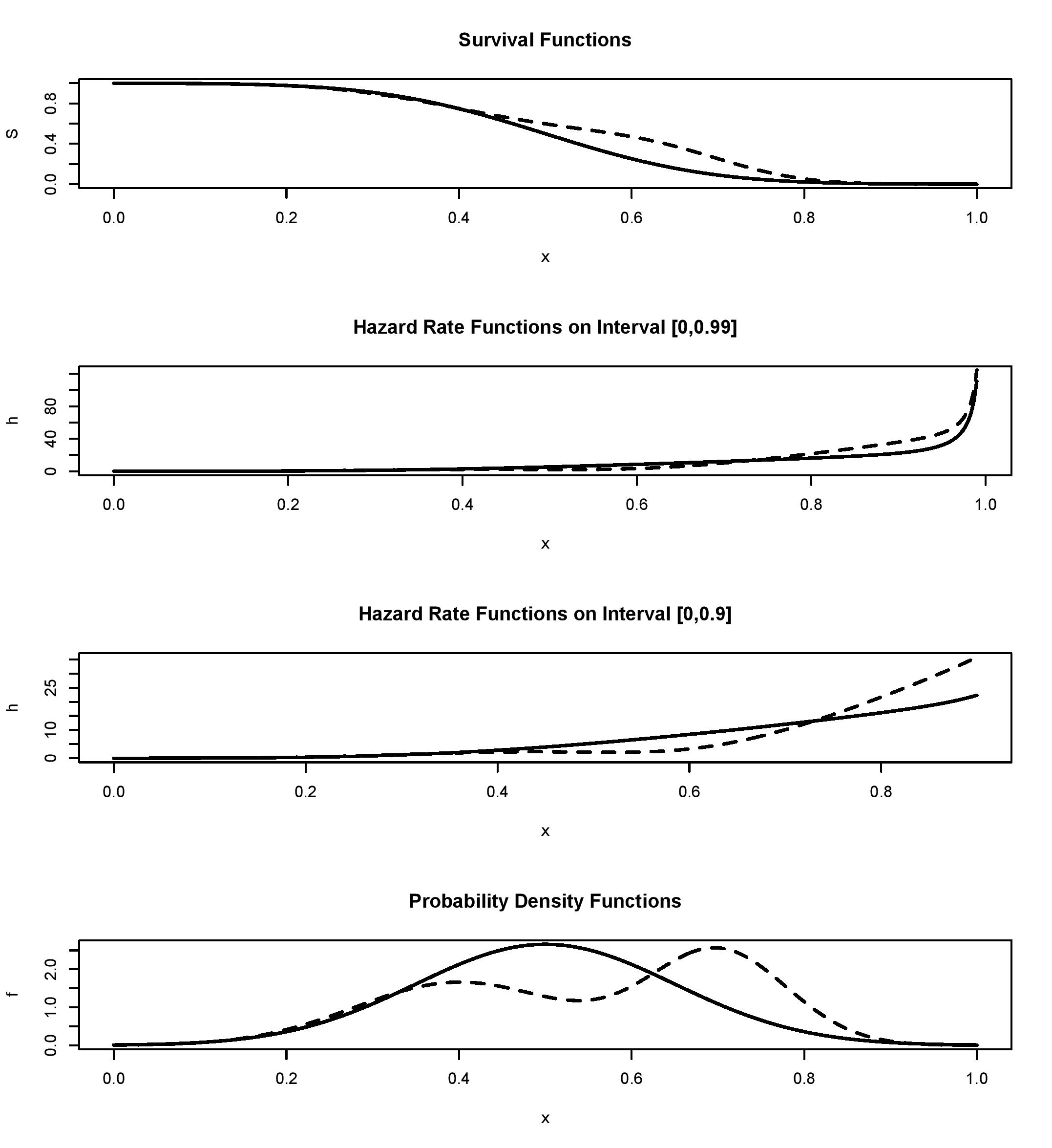
It is instructional to begin with visualization of different characteristics of a random variable used in nonparametric analysis. Figure 1, in its 4 diagrams, exhibits classical characteristics of two random variables supported on and defined in Efromovich (1999, 18). The first one is called the Normal and its a normal distribution truncated onto The second one is called the Bimodal and it is a mixture of two normal distributions truncated onto The top diagram in Figure 1 shows the corresponding survival functions. Can you realize why the solid line corresponds to the Normal and the dashed line to the Bimodal? The answer is likely “no.” We may say that the distributions are primarily different in the area around 0.6 and have a bounded support, but otherwise the cumulative distribution functions are not very instructive. Further, we need dramatically magnify the tails to visually compare them. As a result, in statistics estimates of the cumulative distribution function are primarily used for hypothesis testing about an underlying distribution. The two middle diagrams show the corresponding hazard rates over two different intervals, and please pay attention to scales in the diagrams. Note how dramatically and differently right tails of the hazard rates increase.

Let us explain why a bounded nonnegative variable (and all variables studied in actuarial applications are bounded meaning that for some finite must have a hazard rate that increases to infinity in the right tail. By its definition, the hazard rate of a nonnegative random variable (not necessarily bounded) is a nonnegative function which satisfies the following equality,
\int_0^\infty h^{X^*}(x) dx = \infty. \tag{5.1}
Equality (5.1) follows from (recall (3.11)) and As a result, the right tail of the hazard rate of a bounded random variable always increases to infinity. The latter may be a surprise for some actuaries because familiar examples of hazard rates are the constant hazard rate of an exponential (memoryless) distribution and monotonically decreasing and increasing hazard rates for particular Weibull distributions. Note that these are examples of random variables supported on and in practical applications they are used for approximation of underlying bounded variables.
The fact that the hazard rate of a bounded variable has a right tail that increases to infinity, together with formula (3.9) for the variance of the optimal estimator, indicate that an accurate estimation of the right tail of the hazard rate will be always challenging.
Finally, the bottom diagram in Figure 1 shows us the corresponding probability densities, and now we may realize why they are called the Normal and the Bimodal. Probability density is definitely the most visually appealing characteristic of a continuous random variable.
We may conclude that despite the fact that analytically each characteristic of a random variable may be expressed via another, in a graphic they shed different light on the variable. It is fair to say that in a visual analysis the survival function is the least informative while the density is the most informative and the hazard rate may shed additional light on the right tail. The conclusion is important because in nonparametric statistical analysis graphics are used to visualize data and estimates, see a discussion in Efromovich (1999).

Figure 2 introduces us to the LTRC data and also allows us to look at the reciprocal of the probability which, according to our previous sections, plays a pivotal role in the analysis of LTRC data. The data are simulated and hence we know the underlying distributions. The caption of Figure 2 explains the simulation and the diagrams. The LTRC resembles the “Surgery” example described in the Introduction when the censoring variable may be smaller than the truncation variable. The difference between the two top datasets is in the underlying distributions of We clearly see from these diagrams that the data are left truncated, the latter is indicated by the left edge of datasets created by the inequality The data do not specify how severe the underlying truncation is, at the same time the titles show that from LTRC observations only in the top diagram and in the diagram below are uncensored. We conclude that more than 20% of truncated realizations are censored. Further, we can tell that the support of T is about [0, 0.5] and the support of goes at least from 0 to around 0.94. This allows us to speculate about a severe truncation of the underlying data.
Now let us recall that the hazard rate and density estimates, introduced in the previous sections, use statistics As we will see shortly, these reciprocals exhibited in the bottom diagrams may help us to choose a feasible interval of estimation of the hazard rate and conditional density. The third diagram shows us these reciprocals for all observed while the bottom diagram shows only the reciprocals not exceeding 10. Note the different scales in the two diagrams, how rapidly the tails increase, and that for the Bimodal (the triangles) we can choose a larger interval of estimation than for the Normal (the crosses).
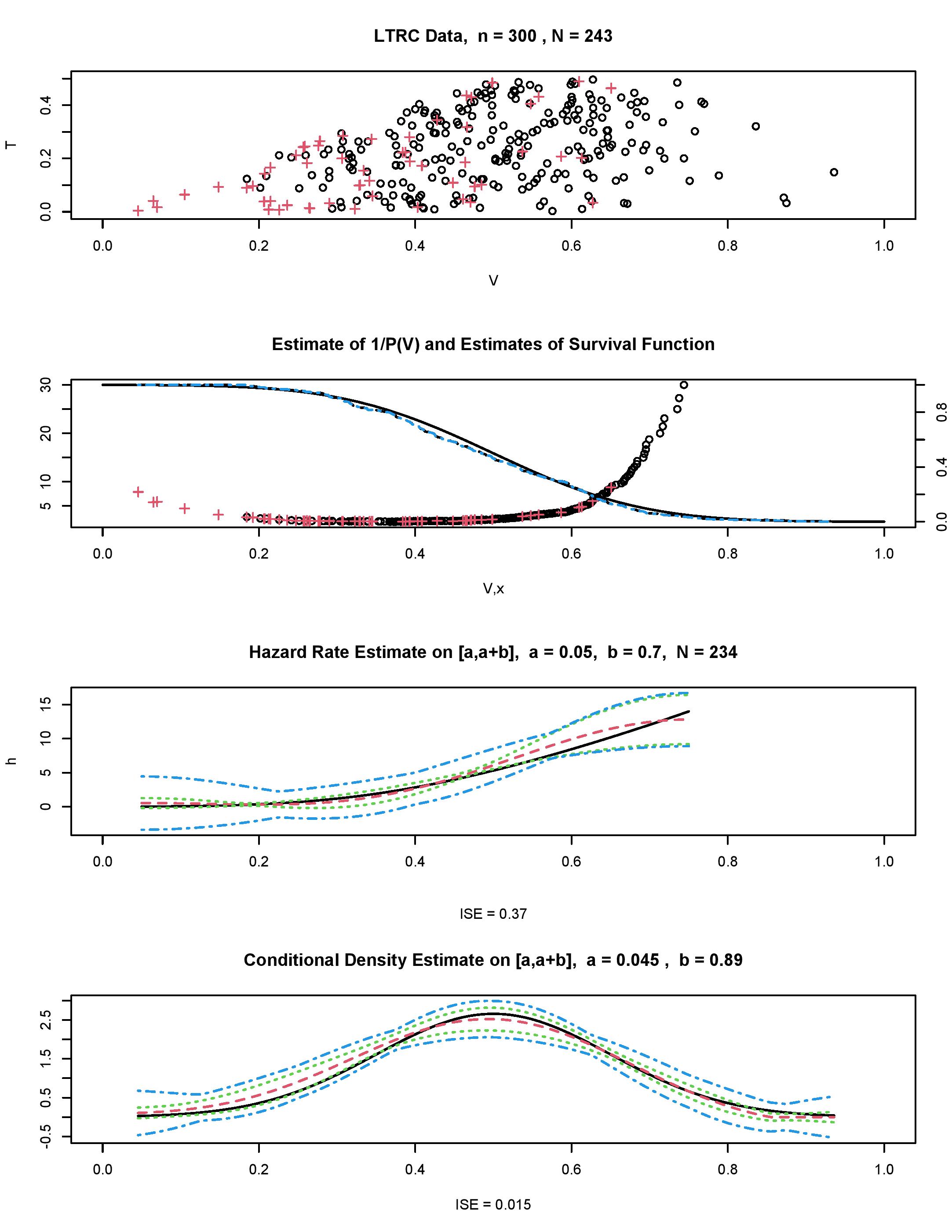
Figure 3, using simulated data, explains how the proposed nonparametric sample mean estimation methodology performs. The top diagram shows us LTRC data which is simulated as in the second diagram in Figure 2 with being the Bimodal. In the diagram we see the familiar left edge created by the truncation. Further, note that there are practically no observations in the tails, and the left tail of observations is solely created by censored observations indicated by the crosses. We may conclude that it will be a complicated task to restore the underlying distribution of interest modified by the LTRC.

Reciprocals that do not exceed 10.5, are shown in the second diagram. Similarly to Figure 2, the circles and crosses correspond to uncensored and censored cases exhibited in the top diagram. The estimates help us to quantify complexity of the problem and choose a reasonable interval of estimation. Also recall that the underlying function is shown by triangles in Figure 2. The second diagram also exhibits the underlying survival function (the solid line) as well as its Kaplan–Meier (the dashed line) and the sample mean (3.12) with (the dotted line) estimates. Note that the corresponding scale is shown on the right vertical axis. The two estimates are practically identical and far from being perfect for the considered sample size and uncensored cases.
The third from the top diagram shows us the proposed estimate of the hazard rate (the dashed line) which, thanks to the simulation, may be compared with the underlying hazard rate (the solid line). The interval of estimation is chosen by considering relatively small values of estimated The integrated squared error ISE=0.29 of the nonparametric estimate is shown in the subtitle. Overall the estimate is good given the large range of its values. The estimate is complemented by pointwise and simultaneous, over the interval of estimation, confidence bands. The bands are symmetric around the estimate to highlight its variance (note that the hazard rate is nonnegative so we could truncate the bands below zero). Together with the estimate the bands help us to choose a feasible interval of estimation.
The fourth from the top diagram shows us an estimate of the hazard rate calculated for the larger interval than in the third diagram. First of all, compare the scales. With respect to the third diagram, the confidence bands are approximately twice wider and the ISE is more than tenfold larger. The pointwise confidence band tells us that the left tail of the hazard rate is still reasonable but the right one may be poor. The chosen interval, and specifically are too large for a reliable estimation. The conclusion is that an interval of estimation should be chosen according to the estimate of and then confirmed by confidence bands.
The bottom diagram in Figure 3 shows estimation of the conditional density. Note that here, as we have predicted in Section 4, the interval of estimation may be larger than for the hazard rate estimation. In particular, for this data it is possible to consider an interval defined by the range of observed values of and then the confidence bands allow us to evaluate feasibility of that choice. The ISE=0.035 indicates that the estimator does a good job. Indeed, the estimate nicely shows the two modes and gradually decreasing tails.

Figure 4 is similar to Figure 3 only here the underlying variable of interest is the Normal (its density is shown in Figure 1) and the censoring is motivated by presented in the Introduction “Home-Insurance” example when the censoring variable is larger than the truncation one (the simulation is explained in the caption). Note that again we have just a few observations in the tails. In particular, there are only 4 observations of larger than 0.8. The left edge of the dataset looks familiar and it indicates a heavy underlying truncation. The hazard rate and conditional density estimates look good but this should be taken with a grain of salt. The estimates correctly show the underlying shapes, but the confidence bands indicate the possibility of a large volatility.
Now, after we have polished our understanding of how to analyze simulated data, let us consider Figure 5 where the auto-losses data from Frees (2009) are explored. The top diagram shows us the histogram of auto-losses scaled onto The histogram is overlaid by our nonparametric estimates of the hazard rate (the horizontal dashed line) and the probability density (the solid line). Note that the two estimates complement each other and none is a plug-in of another, the latter explains their slightly different messages. The hazard rate estimate indicates a possible exponential underlying distribution (recall that this distribution has a constant hazard rate). Let us check this conjecture. First, in the top diagram the dotted line shows us an exponential density with the sample mean rate (note that this is a parametric estimate). Our nonparametric density estimate (the solid line) slowly oscillates around the exponential one. Further, let us add to the diagram the corresponding parametric exponential cumulative distribution function (the long-dashed line) and its empirical estimate (the dot-dashed line). These two curves are multiplied by 6 for better visualization, we may observe a relatively large deviation near and the classical nonparametric Kolmogorov-Smirnov test yields the p-value 0.002 which does not support the conjecture about the exponential distribution. Nonetheless, if we would like to choose a parametric distribution to fit or model the data, then an exponential one may be a fair choice.
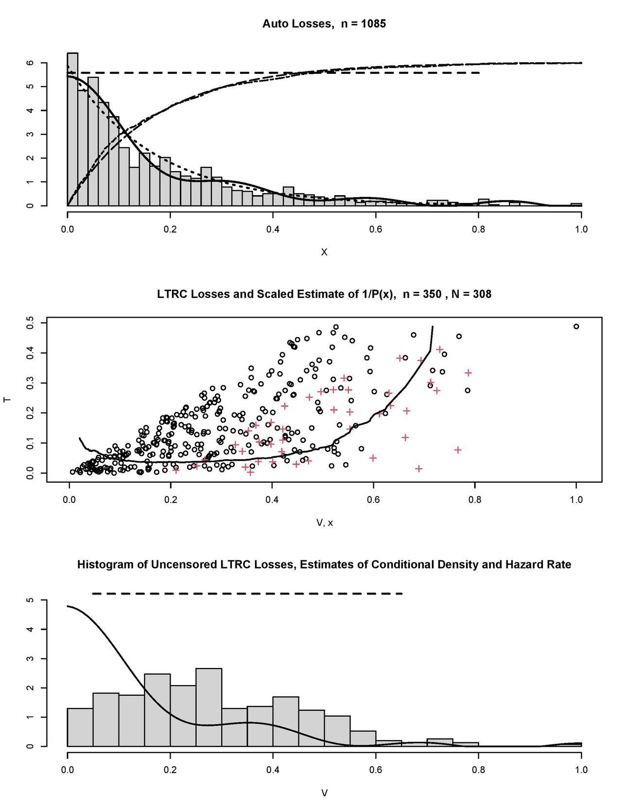
The hazard rate and density estimates, shown in the top diagram of Figure 5, can be considered as benchmarks for any LTRC modification. The middle diagram shows a simulated LTRC modification of the losses, here the truncation variable is Uniform(0,0.5), the censoring variable and is Uniform(0,0.5). Circles and crosses show uncensored and censored losses, respectively. LTRC losses are overlaid by the scaled estimate of (the solid line). We see the pronounced left edge of the truncated data, and notice the devastating truncation of the available observations from 1,085 to only 350 in the LTRC data. Further, among those 350 only 308 are uncensored. Also, look at the right tail where we have just a single observation with larger than 0.8. As we already know, there is no way for us to restore the right tail based on just one observation. The estimated quantifies complexity of the LTRC modification. The bottom diagram shows us the histogram of uncensored realizations of It has no resemblance to the underlying distribution shown in the top diagram, and this histogram explains how the LTRC modifies the data of interest. Note that if the LTRC is ignored, then the histogram in the bottom diagram points to the presumed underlying distribution of losses. The latter clearly would be a mistake. On the other hand, the conditional density estimate (the solid line) and the hazard rate estimate (the dashed line) are good and similar to the benchmarks shown in the top diagram. Keeping in mind the truly devastating truncation and censoring of the underlying losses, the outcome is encouraging.
Figure 6 exhibits a LTRC dataset “channing.” The top diagram shows us available lifetimes. Its left edge looks familiar, and it indicates heavy left truncation. Further, look at how many cases of censoring, shown by crosses, occur at or near the left edge. Further, we are dealing with an extremely heavy right censoring when only 38% of observations are uncensored (the number of uncensored observations is shown in the title). Now let us look at the right edge of the LTRC data. First, note that it is parallel to the left edge. Second, the right edge is solely created by censored observations (shown by crosses). This tells us that the data are based on a study with a specific baseline and a fixed duration. In addition to that, we may say that a large number of observations were censored during the study for reasons other than the end of the study. The heavy LTRC is quantified by the estimated reciprocal of the probability see the solid line in the top diagram. This estimate clearly indicates restrictions on a reliable recovery of tails.

The bottom diagram in Figure 6 allows us to look at the available uncensored observations of exhibited by the histogram. In the histogram we observe two modes with the right one being larger and more pronounced than the left one. The solid line shows us the estimated conditional density. Note how the estimate takes into account the LTRC nature of the data by skewing the modes with respect to the histogram. Recall that we have observed a similar performance in the simulated examples.
Now let us look at another interesting LTRC dataset “centrifuge” presented in Figure 7, the structure of its diagrams is identical to Figure 6. The data, rescaled onto are based on a study of the lifetime of centrifuge’s conveyors used at municipal wastewater treatment plants. Conveyers are subject to abrasive wear (primarily by sand), spare parts are expansive, and repair work is usually performed by the manufacturer. This is why a fair manufacturer’s warranty becomes critical (recall our discussion of warranties in the Introduction). The aim of the study was to estimate the distribution of the lifetime of a conveyor.

First of all, let us look at the available data shown in the top diagram. We see the pronounced right edge of the data created by crosses (censored lifetimes). It indicates the end of the study when all still functioning conveyors are censored. At the same time, only two lifetimes (conveyors) are censored by times smaller than 0.6; this is due to malfunctioning of other parts of the centrifuges. Further, there is no pronounced left edge of the data which is typically created by truncation. These are helpful facts for the considered case of small sample size The top diagram also shows us the estimate of (the solid line), and note that its scale is shown on the right vertical axis. It supports our visual analysis of the data about a minor effect of the truncation and the primary censoring due to end of the study. Also note that there are no observed small lifetimes, and this forces us to consider estimates only for values larger than 0.2.
The bottom diagram in Figure 7 exhibits the hazard rate (the dashed line) and conditional density (the solid line) estimates. Note how the intervals of estimation are chosen according to the estimated shown in the top diagram. The density estimate is informative and it indicates two modes (note how again the estimate takes into account the LTRC modification with respect to the histogram of uncensored lifetimes). There is a plausible explanation of the smaller mode. Some municipal plants use more advanced sand traps, and this may explain the larger lifetimes of conveyors.
Based on the available data we cannot check the above-made conjecture about the underlying origin of the smaller mode, but this issue leads us to a new and important research problem of regression for LTRC data. So far the main approach to solve this problem has been based on multiplicative parametric Cox models, often called the proportional hazards models, see a discussion in Klein and Moeschberger (2003) and Frees (2009). It will be of interest to test the developed sample mean approach for solving the problem of nonparametric regression.
Now let us present results of a numerical study that compares the proposed sample mean estimators with those supported by R. Hazard rate and density estimators are available for censored data in R packages muhaz and survPresmooth, respectively. The numerical study is based on the following Monte Carlo simulations. The underlying distributions are either the Normal or the Bimodal shown in Figure 1, the censoring distributions are either Unif(0, or exponential with the rate (mean) Considered sample sizes are 100, 200, 300, 400, and 500. For each such experiment (i.e., a density, a censoring distribution, and a sample size), 500 Monte Carlo simulations are performed. Then for each experiment the empirical integrated squared error (ISEpl) of the product limit estimator supported by R and the empirical integrated squared error (ISEsm) of the proposed sample mean estimator are calculated. For the hazard rate and the density the integrated squared errors are calculated over intervals and respectively. Then the median ratios (over 500 simulations) of ISEpl/ISEsm are shown in Table 1. Note that the ratio larger than 1 favors the sample mean estimator.
As we see, the sample mean estimators of the hazard rate and the density perform well. Further, because they mimic asymptotically efficient estimators, their relative performance improves for larger sample sizes. Further, the performance of proposed estimators is robust toward changes in censoring distributions.
Conclusion
Left truncation and right censoring are typical data modifications that occur in actuarial practice. Traditionally, the distribution of interest is recovered via a product-limit estimate of the conditional survival function. The present paper advocates complementing this approach with nonparametric sample mean estimation of the hazard rate and the conditional probability density. The attractive feature of the proposed hazard rate estimation is that it is nonparametric, completely data driven, and its sample-mean structure allows us to use a classical statistical inference developed for parametric sample mean estimators. Further, the presented theory shows that the key quantity in understanding what can and cannot be done in restoring an underlying distribution of interest is the probability which is nicely estimable by a sample mean estimator. Presented simulated and real examples explain how to analyze left truncated and censored data and illustrate performance of the proposed nonparametric estimators of the hazard function and conditional probability density.
Main Notations
is the expectation, is the probability of event and is the indicator of event For a random variable denotes its cumulative distribution function (cdf), is the survival function, is the conditional survival function. For a continuous denotes its probability density, is the conditional probability density, is the hazard rate.
is the hidden underlying random variable of interest (the lifetime), is the truncation variable, is the censoring variable. Modified by censoring variables are and the indicator of censoring Given no truncation occurs, that is the available left truncated and right censored (LTRC) triplet is where see definition of the LTRC mechanism in the second paragraph of Section 2. denotes an available sample from In definition (1.3) of the product-limit Kaplan-Meier estimator, denote ordered pairs according to that is
An accent indicates an estimator (statistic). For instance, is the estimator of corresponding Fourier coefficients see (3.5) and (3.6), is an estimator of the survival function etc. In used series estimators, denote elements of the cosine basis on
denotes the probability to avoid truncation, is the pivotal probability in analysis of LTRC, and is the random number of uncensored observations in an LTRC sample.
Acknowledgements
The research is supported in part by a CAS Grant and NSF Grant DMS-1915845. Valuable suggestions by the Editor-in-Chief Dr. Rick Gorvett and two referees are greatly appreciated.