Regression Shrinkage and Selection for Actuarial Models

undefined

1. Introduction

Data arising in actuarial science are typically non-normal, because extremely large losses may arise with small probabilities, whereas small losses may arise with very high probability. For this reason, heavy-tail distributions have been utilized in the literature to capture the nature of highly skewed insurance loss data. An example of a flexible class of distributions to model heavy-tailed data is the GB2 (Generalized Beta of Second Kind) distributions. The density function for the GB2 distribution is shown in Section 3.

In relation to loss models, regression is a useful technique to understand the influence of explanatory variables on a response variable. For example, an actuary may use regression to figure out the average building and contents loss amount for different entity types, by using entity type indicators as explanatory variables in a regression. The actuary may then use the regression coefficient estimates to determine the relationship between the explanatory variables and the response. Performing a regression typically requires an assumption on the distribution of the response variable, and for this reason loss models and regression are closely related, in the actuarial science context.

Now consider the case when there are too many explanatory variables, or in other words when \(\mathbf{x}\) is high dimensional. In this case, estimation of the regression coefficients become a challenging task. In the statistics literature, this problem is solved using so called high dimensional statistical methods, an example of which is the lasso estimation method, see Tibshirani (1996). The lasso approach penalizes the log-likelihood of a regression problem with a penalty term, which reduces the number of coefficients to be estimated. In the statistics literature, lasso methods have been applied extensively to linear regression models, generalized linear models, and recently to the Tweedie distribution (see Qian, Yang, and Zou 2016), which is useful for modeling the pure premium of insurance losses. For example, let \(\ell(\beta_0, \mathbf{\beta})\) be the log-likelihood function for a linear model, where \(\beta_0\) and \(\mathbf{\beta}\) are the regression coefficients to be estimated. In this case, the penalized negative log-likelihood \(- \ell(\beta_0, \mathbf{\beta})/n + P(\beta_0, \mathbf{\beta}, \lambda)\) may be minimized in order to obtain a sparse set of coefficients \(\mathbf{\beta}\), given a tuning parameter \(\lambda\), and a penalty function \(P\). If the group lasso penalty function is used, the regression coefficient becomes

\[(\hat{\beta}_0, \hat{\mathbf{\beta}}) = \mathop{\text{arg min}}_{\beta_0, \mathbf{\beta}} \left\{ - \frac{1}{n} \sum_{i=1}^n\ell(\beta_0, \mathbf{\beta}) \right\} \nonumber + \lambda \sum_{j=1}^g \lVert \mathbf{\beta}_j \lVert_{\mathbf{S}_j^*},\]

where \(\mathbf{x}_i = (\mathbf{x}_{i1}^T, \mathbf{x}_{i2}^T, \dots, \mathbf{x}_{ig}^T)^T\), and \(\mathbf{\beta} = ( \mathbf{\beta}_1^T, \dots, \mathbf{\beta}_g^T)^T\), and \(g\) is the number of groups in the model. Here, \(\lVert \, \cdot \, \lVert_{\mathbf{S}_j^*} = \sqrt{\mathbf{\beta}_j^T \mathbf{S}_j^* \mathbf{\beta}_j}\), with \(\mathbf{S}_j^*\) is a square matrix. Often an identity matrix is used for \(\mathbf{S}_j^*\), resulting in the notation \(\lVert \, \cdot \, \lVert_{2} = \sqrt{\mathbf{\beta}_j^T \mathbf{\beta}_j}\). Extensive work in the statistical learning literature has been performed recently, and the method has become a popular choice for analyzing high-dimensional data in the bio-medical context.

One can easily imagine plugging in the log-likelihood for heavy-tailed loss models, or the log-likelihood for the GB2 distribution in place of \(\ell(\beta_0, \mathbf{\beta})\), in order to obtain a sparse set of coefficients \(\mathbf{\beta}\) for a high-dimensional problem in actuarial science. This is precisely the motivation for this paper. The lasso approach has not been applied to heavy-tailed loss distributions yet in the statistics literature, nor the actuarial literature. In this paper, we will demonstrate how fast regression routines with group-lasso penalties (a variable selection approach for selecting groups of coefficients as in Yuan and Lin 2006) can be built for important loss models including the GB2 distribution.

2. Theory

2.1. One dimensional LASSO

The easiest way to understand a concept is to look at a simple example. Let’s suppose we are interested in minimizing a function as simple as

\[\ell(b) = b^2 \tag{1}\]

By inspection, the minima is \(b=0\). To numerically converge to this solution, we may use Newton’s method. A good overview of numerical methods including Newton’s method is Heath (2002). For the method to work, we need the first and second derivative of the function \(\ell(b)\) evaluated at a particular point, say \(\tilde{b}\). The expressions for the first and second derivatives are simple, and we have \(\ell^\prime(b) = 2b\) and \(\ell^{\prime\prime}(b) = 2\). Then, the update scheme for Newton’s method becomes:

\[\tilde{b}_{(new)} = \tilde{b} - \frac{\ell^\prime(\tilde{b})}{\ell^{\prime\prime}(\tilde{b})} = \tilde{b} - \tilde{b} = 0 \tag{2}\]

where we have converged in one step, because Newton’s method is basically iteratively solving quadratic approximations to the original function, and in this case the original function is quadratic. This procedure can in general be easily implemented on a computer using the following algorithm:

In statistics, or actuarial science practices, the objective function may be defined as a negative log-likelihood function, whose arguments are coefficients of a model to be estimated. Because the likelihood function in such cases are defined as a summation of log likelihood values evaluated at observations of the data, we may imagine that there is some spurious noise in the data related to the argument, resulting in the function to be

\[\ell_\epsilon(b) = (b-\epsilon)^2 \tag{3}\]

where we imagine \(\epsilon>0\) is a small number. The minima of \(\ell_\epsilon(b)\) is \(\epsilon\). Yet, we may not be interested in the effects of the spurious noise. Let’s suppose we are actually interested in the “true” solution \(0\). In order to remove the noise, we may use the LASSO technique, introduced in the statistics literature originally by Tibshirani (1996). The idea is to penalize the likelihood function, so that we minimize the expression

\[\ell_P(b) = \ell_\epsilon(b) + \lambda \cdot |b| \tag{4}\]

for some tuning parameter \(\lambda \ge 0\). Doing this results in a so called shrinkage of the parameter \(b\), so that if \(\lambda\) is large enough and \(\epsilon\) is small enough, the solution returned by the algorithm is indeed the desired \(0\). The tuning parameter basically tells us how strong the penalty should be, where a stronger penalty corresponds to the removal of larger values of \(\epsilon\)’s. Let’s first suppose \({b}\ge0\). Then, equation 4 reduces to

\[\ell_P({b}) = \ell_\epsilon({b}) + \lambda \cdot {b} \tag{5}\]

In this case, the first and second derivatives of the function \(\ell_P(b)\) would be \(\ell_P^\prime({b}) = 2({b}-\epsilon) + \lambda\) and \(\ell_P^\prime({b}) = 2\). Thus, the first order condition gives \(b = \epsilon - \lambda/2\), \(b\ge 0\), whose solution is \(b=0\) if \(\lambda \ge 2 \epsilon\), and a positive number otherwise. If \({b} \le 0\), then a similar thought process gives \(b = \epsilon + \lambda/2 > 0\), which is contradictory. So the solution satisfies:

\[\tilde{b}_{(new)} = \begin{cases} 0 & 2 \epsilon \le \lambda \\ \epsilon - \lambda/2 & \text{ otherwise } \end{cases} \tag{6}\]

If we plot this solution for \(\lambda=1\), we obtain the graph in Figure 1. In the figure, notice that if the spurious noise is large, then the LASSO routine converges to some positive number, but if the noise is small, then it is successful at converging to zero.

2.2. Two dimensional problem

This time, let’s consider the following function:

\[\ell(a,b) = a^2 + b^2 + (a\cdot b)^2 \tag{7}\]

By inspection, the minima is clearly \((0,0)\). For Newton’s method to work, we need the gradient, and the Hessian matrix, of the function evaluated at a particular point, \((\tilde{a}, \tilde{b})^T\). We denote the function value at the point \(\ell(\tilde{a},\tilde{b})\). The gradient and Hessian at the point can be obtained by differentiation:

\[\begin{align} \tilde{\mathbf{U}} &= \begin{pmatrix} 2\tilde{a} + 2\tilde{a}\tilde{b}^2 \\ 2\tilde{b} + 2\tilde{a}^2 \tilde{b} \end{pmatrix} = \begin{pmatrix} \tilde{U}_1 \\ \tilde{U}_2 \end{pmatrix} \\ \tilde{\mathbf{H}} &= \begin{bmatrix} 2 + 2 \tilde{b}^2 & 4\tilde{a}\tilde{b} \\ 4\tilde{a}\tilde{b} & 2 + 2 \tilde{a}^2 \end{bmatrix}= \begin{bmatrix} \tilde{H}_{11} & \tilde{H}_{12} \\ \tilde{H}_{21} & \tilde{H}_{22} \end{bmatrix} \end{align} \tag{8}\]

Then, given an initial guess \((\tilde{a}, \tilde{b})^T\), the updated values may be obtained by

\[\begin{pmatrix} \tilde{a}_{(new)} \\ \tilde{b}_{(new)} \end{pmatrix} = \begin{pmatrix} \tilde{a} \\ \tilde{b} \end{pmatrix} - \tilde{\mathbf{H}}^{-1} \tilde{\mathbf{U}} \tag{9}\]

This procedure can be easily implemented using the following algorithm.

Let’s see what happens now when we have spurious noise in both of the variables \(a\) and \(b\). With spurious noise, the function may be perturbed to

\[\begin{align} \ell_\epsilon(a,b) = \ &(a-\epsilon_a)^2 + (b-\epsilon_b)^2 \\ &+ (a-\epsilon_a)^2(b-\epsilon_b)^2 \end{align} \tag{10}\]

We hope to use the LASSO technique to minimize the expression

\[\ell_P(a,b) = \ell_\epsilon(a,b) + \lambda \cdot \left(|a| + |b|\right) \tag{11}\]

The hope is that we are able to apply first order conditions similar to that in Section 2.1 separately to each of \(a\) and \(b\), but we immediately see that this is not so easy, because the update scheme now involves a matrix multiplication by the Hessian inverse in Equation (9). The hope is that we can ignore the off-diagonal terms of the Hessian matrix and use update schemes like

\[\begin{gathered} \tilde{a}_{(new)} = \tilde{a} - \frac{U_1}{H_{11}}, \quad \tilde{b}_{(new)} = \tilde{b} - \frac{U_2}{H_{22}}\end{gathered} \tag{12}\]

which would allow us to shrink each parameter separately using the same technique as in Section 2.1. Doing this directly, however results in the algorithm to diverge, because it is not a correct Newton’s method. The good news is, by using a double loop, it “kind of” becomes possible to do this! The way it can be done is explained in the next section.

2.3. Double looping

Let’s try to understand how the approach taken in Yang and Zou (2015) and Qian, Yang, and Zou (2016) for the implementation of the gglasso R package, and the HDtweedie package really works. To keep the discussion as simple as possible, let us continue to consider the simple function in Section 2.2. Let

\[\begin{align} \tilde{\mathbf{U}}_\epsilon &= \begin{pmatrix} 2(\tilde{a}-\epsilon_a) + 2(\tilde{a}-\epsilon_a)(\tilde{b}-\epsilon_b)^2 \\ 2(\tilde{b}-\epsilon_b) + 2(\tilde{a}-\epsilon_a)^2 (\tilde{b}- \epsilon_b) \end{pmatrix} \\ &= \begin{pmatrix} \tilde{U}_{\epsilon,1} \\ \tilde{U}_{\epsilon,2} \end{pmatrix} \end{align} \tag{13}\]

\[\tilde{\mathbf{H}}_\epsilon = \begin{bmatrix} 2 + 2 \tilde{b}^2 & 4\tilde{a}\tilde{b} \\ 4\tilde{a}\tilde{b} & 2 + 2 \tilde{a}^2 \end{bmatrix}= \begin{bmatrix} \tilde{H}_{\epsilon,11} & \tilde{H}_{\epsilon,12} \\ \tilde{H}_{\epsilon,21} & \tilde{H}_{\epsilon,22} \end{bmatrix}\tag{14}\]

The idea is to allow the \(\tilde{\mathbf{U}}_\epsilon\) vector and \(\tilde{\mathbf{H}}_\epsilon\) matrix be updated in the outer loop, while running an internal loop that allows the algorithm to converge to each Newton’s method iteration solution for each of the parameters separately. Let’s denote the parameter values in the outer loop \((\tilde{a}, \tilde{b})\). At that current parameter value, we can obtain the \(\tilde{\mathbf{U}}_\epsilon\) vector and \(\tilde{\mathbf{H}}_\epsilon\) matrix. Then, consider the quadratic surface

\[\begin{align} \ell_Q(a,b) = \ &\ell_\epsilon(\tilde{a},\tilde{b}) + \tilde{\mathbf{U}}^T_\epsilon \begin{pmatrix} a - \tilde{a} \\ b - \tilde{b} \end{pmatrix} \\ &+ \frac{1}{2} \begin{pmatrix} a - \tilde{a} \\ b - \tilde{b} \end{pmatrix}^T \tilde{\mathbf{H}}_\epsilon \begin{pmatrix} a - \tilde{a} \\ b - \tilde{b} \end{pmatrix} \end{align} \tag{15}\]

We can think of Newton’s iteration as solving a quadratic minimization problem at each step, and Equation (15) is what this surface looks like in a functional form. Remember that values with the tilde sign are fixed in the outer loop. We have the liberty to solve each Newton iteration step whatever way we want. So let’s consider taking a quadratic approximation to (15) one more time. What this will do is create an inner loop, which will run within each Newton’s method iteration of the outer loop. We have

\[\frac{\partial \ell_Q}{\partial a} = \tilde{U}_{\epsilon,1} + \tilde{H}_{\epsilon,11} ( a - \tilde{a}) + \tilde{H}_{\epsilon,12} ( b - \tilde{b}) \tag{16}\]

\[\frac{\partial \ell_Q}{\partial b} = \tilde{U}_{\epsilon,2} + \tilde{H}_{\epsilon,22} ( b - \tilde{b}) + \tilde{H}_{\epsilon,12} ( a - \tilde{a}) \tag{17}\]

and second derivatives

\[\begin{align} \frac{\partial^2 \ell_Q}{\partial a^2} = \tilde{H}_{\epsilon,11}, &\quad \frac{\partial^2 \ell_Q}{\partial a \partial b} = \tilde{H}_{\epsilon,12}, \\ \quad \frac{\partial^2 \ell_Q}{\partial b^2} &= \tilde{H}_{\epsilon,22} \end{align} \tag{18}\]

Denote

\[\mathbf{U}_Q = \begin{pmatrix} \frac{\partial \ell_Q}{\partial a} & \frac{\partial \ell_Q}{\partial b} \end{pmatrix}^T, \quad \mathbf{H}_Q = \begin{bmatrix} \tilde{H}_{\epsilon,11} & \tilde{H}_{\epsilon,12} \\ \tilde{H}_{\epsilon,21} & \tilde{H}_{\epsilon,22} \end{bmatrix} \tag{19}\]

From here, we assume that we are given the current estimate for the inner loop, \((\breve{a},\breve{b})\), starting from \((\tilde{a},\tilde{b})\). Our goal is to minimize \(\ell_Q\). Consider updating \(\breve{a}\) separately, and \(\breve{b}\) separately. Consider \(\tilde{a}\) for example. Fixing the value of \(b\) to \(\tilde{b}\), we have

\[\begin{pmatrix} a - \tilde{a} \\ b - \tilde{b} \end{pmatrix} = \begin{pmatrix} a - \tilde{a} \\ 0 \end{pmatrix}, \quad \text{ since } b = \tilde{b} \tag{20}\]

so that we may update \(\breve{a}\) by letting it be

\[\begin{align} \mathop{\text{arg min}}_a ~ &\ell_Q(\tilde{a},\tilde{b}) + \breve{\mathbf{U}}_Q^T \begin{pmatrix} a - \tilde{a} \\ {b} - \tilde{b} \end{pmatrix} \\ &+ \frac{1}{2} \begin{pmatrix} a - \tilde{a} \\ {b} - \tilde{b} \end{pmatrix}^T \mathbf{H}_Q \begin{pmatrix} a - \tilde{a} \\ {b} - \tilde{b} \end{pmatrix} \end{align} \tag{21}\]

which boils down to

\[\begin{align} \mathop{\text{arg min}}_a ~ &\ell_Q(\tilde{a},\tilde{b}) + \breve{U}_{Q,1} (a - \tilde{a}) \\ &+ \frac{1}{2} \tilde{H}_{\epsilon,11} (a - \tilde{a})^2 \end{align} \tag{22}\]

where we have denoted the first component of \(\tilde{\mathbf{U}}_Q\) as \(\tilde{U}_{Q,1}\). The first order condition is

\[\breve{a}_{(new)} = \breve{a} - \frac{\breve{U}_{Q,1}}{\tilde{H_{\epsilon,11}}} \tag{23}\]

A similar procedure for the second parameter gives the first order condition

\[\breve{b}_{(new)} = \breve{b} - \frac{\breve{U}_{Q,2}}{\tilde{H_{\epsilon,22}}} \tag{24}\]

where \(U_{Q,2}\) denotes the second component of \(\mathbf{U}_Q\). Each update is guaranteed to move in a direction in which the \(\ell_Q\) function decreases. Summarizing these steps gives algorithm 3.

2.4. Double looping with penalization

Once we have algorithm 3 working, it takes minimal effort to write a routine that applies LASSO separately to each parameter \(a\) and \(b\). The solutions satisfy:

\[\begin{align} \breve{a}_{(new)} = \ &\left(\tilde{H}_{\epsilon, 11} \times \breve{a} - \breve{U}_{Q,1}\right) \\ &\cdot \frac{\left( 1 - \frac{\lambda}{|\tilde{H}_{\epsilon, 11} \times \breve{a} - \breve{U}_{Q,1}|} \right)_{+} } {\tilde{H}_{\epsilon, 11}} \nonumber \\ = \ & \begin{cases} \breve{a} - \frac{\breve{U}_{Q,1}}{\tilde{H}_{\epsilon,11}} - \frac{\lambda}{\tilde{H}_{\epsilon,11}} \\ \quad\quad \text{if } ~ \breve{a} - \frac{\breve{U}_{Q,1}}{\tilde{H}_{\epsilon, 11}} > \frac{\lambda}{\tilde{H}_{\epsilon, 11}} \\ \breve{a} - \frac{\breve{U}_{Q,1}}{\tilde{H}_{\epsilon,11}} + \frac{\lambda}{\tilde{H}_{\epsilon,11}} \\ \quad\quad \text{if } ~ \breve{a} - \frac{\breve{U}_{Q,1}}{\tilde{H}_{\epsilon, 11}} < - \frac{\lambda}{\tilde{H}_{\epsilon, 11}} \\ 0 \quad\ \ \text{otherwise } \end{cases} \end{align} \tag{25}\]

\[\begin{align} \breve{b}_{(new)} = \ & \left(\tilde{H}_{\epsilon, 22} \times \breve{b} - \breve{U}_{Q,2}\right) \\ &\cdot \frac{\left( 1 - \frac{\lambda}{|\tilde{H}_{\epsilon, 22} \times \breve{b} - \breve{U}_{Q,2}|} \right)_{+} } {\tilde{H}_{\epsilon, 22}} \nonumber \\ = \ &\begin{cases} \breve{b} - \frac{\breve{U}_{Q,2}}{\tilde{H}_{\epsilon,22}} - \frac{\lambda}{\tilde{H}_{\epsilon,22}} \\ \quad\quad \text{if } ~ \breve{b} - \frac{\breve{U}_{Q,2}}{\tilde{H}_{\epsilon, 22}} > \frac{\lambda}{\tilde{H}_{\epsilon, 22}} \\ \breve{b} - \frac{\breve{U}_{Q,2}}{\tilde{H}_{\epsilon,22}} + \frac{\lambda}{\tilde{H}_{\epsilon,22}} \\ \quad\quad \text{if } ~ \breve{b} - \frac{\breve{U}_{Q,2}}{\tilde{H}_{\epsilon, 22}} < - \frac{\lambda}{\tilde{H}_{\epsilon, 22}} \\ 0 \quad\ \ \text{otherwise } \end{cases} \end{align} \tag{26}\]

The new algorithm is the following:

Sparsity would be induced into the resulting final coefficients \(\hat{a}\) and \(\hat{b}\). This principle can be applied to regression models involving a response and explanatory variables \(\mathbf{x}\) and corresponding coefficients \(\mathbf{\beta}\), with responses following distributions found in actuarial science.

2.5. Majorization minimization

In this section, the concept of majorization minimization will be explained. The majorization minimization approach has been introduced into the statistics literature by Lange, Hunter, and Yang (2000), Hunter and Lange (2004), Wu and Lange (2010), and Yang and Zou (2015). In this section, the majorization minimization approach will be demonstrated using a specific problem, so that it is clear why it is needed for the purpose of this paper. Suppose we have observations \(y_1, y_2, \cdots, y_n\), sampled from a Burr distribution with unknown parameters. The Burr distribution has density

\[\begin{align} f(y; \alpha, \gamma, \theta) = \frac{\alpha \gamma (y/\theta)^{\gamma}}{ y [1 + (y/\theta)^\gamma]^{\alpha+1}}, \\ y>0, \alpha>0, \gamma>0, \theta>0 \end{align} \tag{27}\]

The log likelihood function is

\[\begin{align} \ell(\alpha,\gamma,\theta) = -\sum_{i=1}^n \biggl[ &\log(\alpha) + \log(\gamma) + \gamma \log \left(\frac{y_i}{\theta}\right) \\ &- \log(y_i) - (\alpha+1) \\ &\times \log \left( 1 + \left(\frac{y_i}{\theta}\right)^\gamma \right) \biggr] \end{align} \tag{28}\]

The gradient can be obtained by differentiation:

\[\frac{\partial \ell}{\partial \alpha} = - \sum_{i=1}^n \left[ \frac{1}{\alpha} - \log \left( 1 + \left( \frac{y_i}{\theta} \right)^\gamma \right) \right] \tag{29}\]

\[\begin{align} \frac{\partial \ell}{\partial \gamma} = - \sum_{i=1}^n \biggl[ &\frac{1}{\gamma} + \log \left( \frac{y_i}{\theta} \right) - (\alpha+1) \\ &\times \left( \frac{\log(y_i/\theta)}{ 1 + (y_i/\theta)^{-\gamma} } \right) \biggr] \end{align} \tag{30}\]

\[\frac{\partial \ell}{\partial \theta} = - \sum_{i=1}^n \left[ - \frac{\gamma}{\theta} + \frac{\gamma (\alpha+1)}{\theta} \left( \frac{1}{ 1 + (y_i/\theta)^{-\gamma} } \right) \right] \tag{31}\]

The terms for the Hessian can be obtained by differentiation as well:

\[\frac{\partial^2 \ell}{\partial \alpha^2} = \sum_{i=1}^n \frac{1}{\alpha^2} \tag{32}\]

\[\begin{align} \frac{\partial^2 \ell}{\partial \gamma^2} = - \sum_{i=1}^n \Bigg[ &- \frac{1}{\gamma^2} - (\alpha+1) \left[ \log(y_i/\theta) \right]^2 \\ &\times \left[ 1 + (y_i/\theta)^{-\gamma}\right]^{-2} (y_i/\theta)^{-\gamma} \Bigg] \end{align} \tag{33}\]

\[\begin{align} \frac{\partial^2 \ell}{\partial \theta^2} = - \sum_{i=1}^n \Bigg\lbrack &\frac{\gamma}{\theta^2} - \frac{(\alpha+1) \gamma}{\theta^2} \left( \frac{1}{1 + (y_i/\theta)^{-\gamma}} \right) \\ &- (\alpha+1) \left( \frac{\gamma}{\theta} \right)^2 \\ &\times \left[ 1 + \left(\frac{y_i}{\theta} \right)^{-\gamma} \right]^{-2} \left( \frac{y_i}{\theta} \right)^{-\gamma} \Bigg\rbrack \end{align} \tag{34}\]

\[\frac{\partial^2 \ell}{\partial \alpha \partial \gamma} = \sum_{i=1}^n \frac{\log(y_i/\theta)}{ 1 + (y_i/\theta)^{-\gamma} } \tag{35}\]

\[\frac{\partial^2 \ell}{\partial \alpha \partial \theta} = - \sum_{i=1}^n \frac{\gamma}{\theta} \left( \frac{1}{ 1 + (y_i/\theta)^{-\gamma} } \right) \tag{36}\]

\[\begin{align} \frac{\partial^2 \ell}{\partial \gamma \partial \theta} = - \sum_{i=1}^n \Bigg[ &- \frac{1}{\theta} - (\alpha+1) \bigl\{-(1/\theta) \\ &\times \left[ 1 + (y_i/\theta)^{-\gamma} \right] \\ &- \gamma \log(y_i/\theta) (y_i/\theta)^{-\gamma} (1/\theta)\bigr\} \\ &\div \left[ 1 + (y_i/\theta)^{-\gamma} \right]^2 \Bigg] \end{align} \tag{37}\]

From here, in order to ensure the estimated parameters are positive, we use the following re-parameterization of \(\alpha, \gamma\), and \(\theta\):

\[\alpha = \exp(a), \quad \gamma = \exp(b), \quad \theta = \exp(c) \tag{38}\]

Then define

\[\mathbf{U} = \begin{pmatrix} \frac{\partial \ell}{\partial \alpha} \cdot \frac{\partial \alpha}{\partial a} \\ \frac{\partial \ell}{\partial \gamma} \cdot \frac{\partial \gamma}{\partial b} \\ \frac{\partial \ell}{\partial \theta} \cdot \frac{\partial \theta}{\partial c} \end{pmatrix} = \begin{pmatrix} \frac{\partial \ell}{\partial \alpha} \cdot \alpha \\ \frac{\partial \ell}{\partial \gamma} \cdot \gamma \\ \frac{\partial \ell}{\partial \theta} \cdot \theta \end{pmatrix} = \begin{pmatrix} U_1 \\ U_2 \\ U_3 \end{pmatrix} \tag{39}\]

and

\[\begin{align} &\mathbf{H} = \\ &\begin{bmatrix} \frac{\partial^2 \ell}{\partial \alpha^2} \! \cdot \! \left(\frac{\partial \alpha}{\partial a}\right)^2 & \frac{\partial^2 \ell}{\partial \alpha \partial \gamma} \! \cdot \! \frac{\partial \alpha}{\partial a} \! \cdot \! \frac{\partial \gamma}{\partial b} & \frac{\partial^2 \ell}{\partial \alpha \partial \theta} \! \cdot \! \frac{\partial \alpha}{\partial a} \! \cdot \! \frac{\partial \theta}{\partial c} \\ \frac{\partial^2 \ell}{\partial \gamma \partial \alpha} \! \cdot \! \frac{\partial \gamma}{\partial b} \! \cdot \! \frac{\partial \alpha}{\partial a} & \frac{\partial^2 \ell}{\partial \gamma^2} \! \cdot \! \left(\frac{\partial \gamma}{\partial b} \right)^2& \frac{\partial^2 \ell}{\partial \gamma \partial \theta} \! \cdot \! \frac{\partial \gamma}{\partial b} \! \cdot \! \frac{\partial \theta}{\partial c} \\ \frac{\partial^2 \ell}{\partial \theta \partial \alpha} \! \cdot \! \frac{\partial \theta}{\partial c} \! \cdot \! \frac{\partial \alpha}{\partial a} & \frac{\partial^2 \ell}{\partial \theta \partial \gamma} \! \cdot \! \frac{\partial \theta}{\partial c} \! \cdot \! \frac{\partial \gamma}{\partial b} & \frac{\partial^2 \ell}{\partial \theta^2} \! \cdot \! \left( \frac{\partial \theta}{\partial c} \right)^2 \end{bmatrix} \\ & = \begin{bmatrix} \frac{\partial^2 \ell}{\partial \alpha^2} \cdot \alpha^2 & \frac{\partial^2 \ell}{\partial \alpha \partial \gamma} \cdot \alpha \gamma & \frac{\partial^2 \ell}{\partial \alpha \partial \theta} \cdot \alpha \theta \\ \frac{\partial^2 \ell}{\partial \gamma \partial \alpha} \cdot \gamma \alpha & \frac{\partial^2 \ell}{\partial \gamma^2} \cdot \gamma^2& \frac{\partial^2 \ell}{\partial \gamma \partial \theta} \gamma \theta \\ \frac{\partial^2 \ell}{\partial \theta \partial \alpha} \cdot \theta \alpha & \frac{\partial^2 \ell}{\partial \theta \partial \gamma} \cdot \theta \gamma & \frac{\partial^2 \ell}{\partial \theta^2} \cdot \theta^2 \end{bmatrix} \\ &= \begin{bmatrix} H_{11} & H_{12} & H_{13} \\ H_{21} & H_{22} & H_{23} \\ H_{31} & H_{32} & H_{33} \end{bmatrix} \end{align} \tag{40}\]

The second order Taylor’s expansion around a point \((\tilde{a},\tilde{b},\tilde{c})\) is:

\[\begin{align} \ell_Q(a,b,c) = \ &\ell(\tilde{a},\tilde{b},\tilde{c}) + \tilde{\mathbf{U}}^T \begin{pmatrix} a - \tilde{a} \\ b - \tilde{b} \\ c - \tilde{c} \end{pmatrix} \\ &+ \frac{1}{2} \begin{pmatrix} a - \tilde{a} \\ b - \tilde{b} \\ c - \tilde{c} \end{pmatrix}^T \tilde{\mathbf{H}} \begin{pmatrix} a - \tilde{a} \\ b - \tilde{b} \\ c - \tilde{c} \end{pmatrix} \end{align} \tag{41}\]

where \(\tilde{\mathbf{U}}\) and \(\tilde{\mathbf{H}}\) are the gradient and Hessian evaluated at the point. After some simplification, we can differentiate \(\ell_Q\) in order to obtain a double-loop iteration scheme for the estimation of the coefficients. For now let’s assume there is no penalty.

\[\begin{align} &\mathbf{U}_Q = \begin{pmatrix} \frac{\partial \ell_Q}{\partial a} \\ \frac{\partial \ell_Q}{\partial b} \\ \frac{\partial \ell_Q}{\partial c} \end{pmatrix} = \\ &\begin{pmatrix} \tilde{U}_1 + \tilde{H}_{11} (a - \tilde{a}) + \tilde{H}_{12} (b-\tilde{b}) + \tilde{H}_{13} (c - \tilde{c}) \\ \tilde{U}_2 + \tilde{H}_{22} (b - \tilde{b}) + \tilde{H}_{12} (a-\tilde{a}) + \tilde{H}_{23} (c - \tilde{c}) \\ \tilde{U}_3 + \tilde{H}_{33} (c - \tilde{c}) + \tilde{H}_{13} (a-\tilde{a}) + \tilde{H}_{23} (b - \tilde{b}) \end{pmatrix} \end{align} \tag{42}\]

and

\[\mathbf{H}_Q = \begin{bmatrix} \tilde{H}_{11} & \tilde{H}_{12} & \tilde{H}_{13} \\ \tilde{H}_{21} & \tilde{H}_{22} & \tilde{H}_{23} \\ \tilde{H}_{31} & \tilde{H}_{32} & \tilde{H}_{33} \end{bmatrix} \tag{43}\]

We attempt to solve

\[\begin{align} \mathop{\text{arg min}}_{(a,b,c)} \ &\ell_Q(\breve{a},\breve{b},\breve{c}) + \breve{\mathbf{U}}_Q^T \begin{pmatrix} a - \breve{a} \\ b - \breve{b} \\ c - \breve{c} \end{pmatrix} \\ &+ \frac{1}{2} \begin{pmatrix} a - \breve{a} \\ b - \breve{b} \\ c - \breve{c} \end{pmatrix}^T \mathbf{H}_Q \begin{pmatrix} a - \breve{a} \\ b - \breve{b} \\ c - \breve{c} \end{pmatrix} \end{align} \tag{44}\]

Using these, we may attempt to write a naive double-loop iteration scheme to estimate the parameters for the Burr distribution:

The reader would be surprised to learn that Algorithm 5 does not converge in general. Testing it with a randomly generated sample of 5,000 observations from a Burr distribution with parameters \(\alpha=2\), \(\gamma=4\), and \(\theta=1,000\) fails to converge for initial values moderately different from the true parameters. It is basically a three dimensional Newton’s method for \(\ell_Q\) in the inner loop, but the problem is the procedure requires certain conditions on the objective function and the initial values in order for convergence to be guaranteed, which may not hold in general. In order to make the algorithm more stable, we majorize the function within each iteration of the inner loop. Let \(\xi_Q\) be the largest eigen value of \(\mathbf{H}_Q\). Then, instead of Equation (44), we attempt to solve

\[\begin{align} & (\breve{a}_{(new)},\breve{b}_{(new)},\breve{c}_{(new)}) \nonumber \\ & = \mathop{\text{arg min}}_{(a,b,c)} \ell_Q(\breve{a},\breve{b},\breve{c}) + \breve{\mathbf{U}}_Q^T \begin{pmatrix} a - \breve{a} \\ b - \breve{b} \\ c - \breve{c} \end{pmatrix} \\ &\quad \quad\quad\quad + \frac{\xi_Q}{2} \begin{pmatrix} a - \breve{a} \\ b - \breve{b} \\ c - \breve{c} \end{pmatrix}^T \begin{pmatrix} a - \breve{a} \\ b - \breve{b} \\ c - \breve{c} \end{pmatrix} \end{align} \tag{45}\]

The first order condition derived from Equation (45) is used to write the following algorithm. Algorithm 6 converges, and is much more stable:

Algorithm 6 is identical to Algorithm 5 except that the largest eigen value of \(\mathbf{H}_Q\) is used to determine the update. The reason why each step results in a reduction of the objective function in Algorithm 6 is because we have:

\[\begin{align} & \ell_Q(\breve{a}_{(new)},\breve{b}_{(new)},\breve{c}_{(new)}) \nonumber \\ & = \ell(\breve{a},\breve{b},\breve{c}) + \breve{\mathbf{U}}_Q^T \begin{pmatrix} \breve{a}_{(new)} - \breve{a} \\ \breve{b}_{(new)} - \breve{b} \\ \breve{c}_{(new)} - \breve{c} \end{pmatrix} \\ &\quad + \frac{1}{2} \begin{pmatrix} \breve{a}_{(new)} - \breve{a} \\ \breve{b}_{(new)} - \breve{b} \\ \breve{c}_{(new)} - \breve{c} \end{pmatrix}^T \mathbf{H}_Q \begin{pmatrix} \breve{a}_{(new)} - \breve{a} \\ \breve{b}_{(new)} - \breve{b} \\ \breve{c}_{(new)} - \breve{c} \end{pmatrix} \nonumber \\ & \le \ell(\breve{a},\breve{b},\breve{c}) + \breve{\mathbf{U}}_Q^T \begin{pmatrix} \breve{a}_{(new)} - \breve{a} \\ \breve{b}_{(new)} - \breve{b} \\ \breve{c}_{(new)} - \breve{c} \end{pmatrix} \\ &\quad + \frac{\xi_Q}{2} \begin{pmatrix} \breve{a}_{(new)} - \breve{a} \\ \breve{b}_{(new)} - \breve{b} \\ \breve{c}_{(new)} - \breve{c} \end{pmatrix}^T \begin{pmatrix} \breve{a}_{(new)} - \breve{a} \\ \breve{b}_{(new)} - \breve{b} \\ \breve{c}_{(new)} - \breve{c} \end{pmatrix} \nonumber \\ & \le \ell_Q(\breve{a},\breve{b},\breve{c}) \end{align} \tag{46}\]

where the first inequality in Equation (46) holds because of the majorization, and the second inequality holds because \((\breve{a}_{(new)},\breve{b}_{(new)},\breve{c}_{(new)})\) is obtained by solving Equation (45). Thus, \(\ell_Q\) is reduced by the update.

3. Shrinkage and selection for GB2

In this section, the intuitions from Section 2 are applied to the GB2 regression model. We assume that a sample of continuous responses \(y_1, \cdots, y_n\), along with covariates \(\mathbf{x}_1, \cdots \mathbf{x}_n\) are observed. Our goal is to regress the response onto the covariates, assuming the response follows a GB2 distribution. The density for the GB2 distribution is

\[\begin{align} \text{f}_Y(y; a,b, \alpha_1, \alpha_2) = \frac{|a| (y/b)^{a \cdot \alpha_1}}{y B(\alpha_1, \alpha_2) [1+(y/b)^a]^{\alpha_1+\alpha_2} }, \\ 0 < y < \infty. \end{align}\]

The GB2 distribution has been applied extensively to solving insurance ratemaking problems in the actuarial literature recently. For regression purposes, it is helpful to reparameterize the density. Following Frees, Lee, and Yang (2016), and Sun, Frees, and Rosenberg (2008), we define:

\[\begin{align} \text{f}_{Y}(y; \mu,\sigma,\alpha_1,\alpha_2) = \frac{[\text{exp}(z)]^{\alpha_1}}{y\sigma B(\alpha_1,\alpha_2)[1+\text{exp}(z)]^{\alpha_1+\alpha_2}} \\ \text{ for } 0 < y < \infty \end{align}\]

where the parameterization for regression is

\[\begin{align} z = \frac{\text{ln}(y)-\mu}{\sigma}, &\quad \mu = \beta_0 + \mathbf{x}^T \mathbf{\beta}, \\ a = 1/\sigma, &\quad b = \exp(\mu). \end{align} \tag{47}\]

With this, we can write the negative log-likelihood to be maximized:

\[\ell(\beta_0, \mathbf{\beta}, \sigma, \alpha_1, \alpha_2) = \sum_{i=1}^n \Phi(y_i, \mu_i) \tag{48}\]

where

\[\begin{align} \Phi(y_i, \mu_i) = \ &\log(y_i) + \log(\sigma) + \log B(\alpha_1, \alpha_2) \nonumber \\ & + (\alpha_1 + \alpha_2) \\ &\times \log \left( 1 + \exp \left( \frac{\ln(y_i) - \mu_i}{\sigma} \right) \right) \\ &- \alpha_1 \left( \frac{\ln(y_i) - \mu_i}{\sigma} \right).\end{align} \tag{49}\]

and

\[\begin{align} B(\alpha_1, \alpha_2) = \frac{\Gamma(\alpha_1) \Gamma(\alpha_2)}{\Gamma( \alpha_1 + \alpha_2 )}\end{align} \tag{50}\]

In order to take the approach in Section 2.4, we need the gradient and Hessian for the log-likelihood. For this we may differentiate \(\Phi(y_i, \mu_i)\), so that we have

\[\begin{align} \frac{\partial \Phi(y_i, \mu_i)}{\partial \mu_i} = \ &- \left( \frac{\alpha_1 + \alpha_2}{\sigma} \right) \\ &\times \left[ 1 + \exp \left( \frac{\mu_i - \ln(y_i)}{\sigma} \right) \right]^{-1} \\ &+ \frac{\alpha_1}{\sigma}\end{align} \tag{51}\]

\[\begin{align} \frac{\partial \Phi(y_i, \mu_i)}{\partial \sigma} = \ &\frac{1}{\sigma} + (\alpha_1 + \alpha_2) \\ &\times \left[ 1 + \exp \left( \frac{\mu_i - \ln(y_i)}{\sigma} \right) \right]^{-1} \\ &\times \left( \frac{\mu_i - \ln(y_i)}{\sigma^2} \right) \nonumber \\ & - \alpha_1 \left( \frac{\mu_i - \ln(y_i)}{\sigma^2} \right) \end{align} \tag{52}\]

\[\begin{align} \frac{\partial \Phi(y_i, \mu_i)}{\partial \alpha_1} = \ &\psi(\alpha_1) - \psi(\alpha_1 + \alpha_2) \\ &+ \log \left( 1 + \exp \left( \frac{\mu_i - \ln(y_i)}{\sigma} \right) \right) \nonumber \\ &- \left( \frac{\mu_i - \ln(y_i)}{\sigma} \right)\end{align} \tag{53}\]

\[\begin{align} \frac{\partial \Phi(y_i, \mu_i)}{\partial \alpha_2} = \ &\psi(\alpha_2) - \psi(\alpha_1 + \alpha_2) \\ &+ \log \left( 1 + \exp \left( \frac{\mu_i - \ln(y_i)}{\sigma} \right) \right),\end{align} \tag{54}\]

where \(\psi(x) = \frac{d}{dx} \ln \Gamma(x)\) is the digamma function. Next, we obtain the expressions for the Hessian. We have the following second derivative terms:

\[\begin{align} \frac{\partial^2 \Phi(y_i, \mu_i)}{\partial \mu_i^2} = \ &\left( \frac{\alpha_1 + \alpha_2}{\sigma^2} \right) \\ &\times \left[ 1 + \exp \left( \frac{\mu_i - \ln(y_i)}{\sigma} \right) \right]^{-2} \\ &\times \exp \left( \frac{\mu_i - \ln(y_i)}{\sigma} \right)\end{align} \tag{55}\]

\[\begin{align} \frac{\partial^2 \Phi(y_i, \mu_i)}{\partial \sigma \partial \mu_i} = \ &- \frac{\alpha_1 + \alpha_2}{\sigma} \\ &\times \left[ 1 + \exp \left( \frac{\mu_i - \ln(y_i)}{\sigma} \right) \right]^{-2} \\ &\times \exp \left( \frac{\mu_i - \ln(y_i)}{\sigma} \right) \\ &\times \left( \frac{\mu_i - \ln(y_i)}{\sigma^2} \right) \nonumber \\ &+ \frac{\alpha_1 + \alpha_2}{\sigma^2} \\ &\times \left[ 1 + \exp \left( \frac{\mu_i - \ln(y_i)}{\sigma} \right) \right]^{-1} \\ &- \frac{\alpha_1}{\sigma^2} \end{align} \tag{56}\]

\[\begin{align} &\frac{\partial^2 \Phi(y_i, \mu_i)}{\partial \alpha_1 \partial \mu_i} \\ &= - \frac{1}{\sigma} \left[ 1 + \exp \left( \frac{\mu_i - \ln(y_i)}{\sigma} \right) \right]^{-1} + \frac{1}{\sigma}\end{align} \tag{57}\]

\[\begin{align} \frac{\partial^2 \Phi(y_i, \mu_i)}{\partial \alpha_2 \partial \mu_i} & = - \frac{1}{\sigma} \left[ 1 + \exp \left( \frac{\mu_i - \ln(y_i)}{\sigma} \right) \right]^{-1}\end{align} \tag{58}\]

\[\begin{align} \frac{\partial^2 \Phi(y_i, \mu_i)}{\partial \alpha_1 \partial \sigma} = \ &\left[ 1 + \exp \left( \frac{\mu_i - \ln(y_i)}{\sigma} \right) \right]^{-1} \\ &\times \left( \frac{\mu_i - \ln(y_i)}{\sigma^2} \right) \\ &- \left( \frac{\mu_i - \ln(y_i)}{\sigma^2} \right)\end{align} \tag{59}\]

\[\begin{align} \frac{\partial^2 \Phi(y_i, \mu_i)}{\partial \alpha_2 \partial \sigma} = \ &\left[ 1 + \exp \left( \frac{\mu_i - \ln(y_i)}{\sigma} \right) \right]^{-1} \\ &\times \left( \frac{\mu_i - \ln(y_i)}{\sigma^2} \right)\end{align} \tag{60}\]

\[\begin{align} \frac{\partial^2 \Phi(y_i, \mu_i)}{\partial \alpha_1 \partial \alpha_2} & = - \psi_1(\alpha_1 + \alpha_2)\end{align} \tag{61}\]

\[\begin{align} \frac{\partial^2 \Phi(y_i, \mu_i)}{\partial \sigma^2} = \ &(\alpha_1 + \alpha_2) \\ &\times \left[ 1 + \exp \left( \frac{\mu_i - \ln(y_i)}{\sigma} \right) \right]^{-2} \\ &\times \exp \left( \frac{\mu_i - \ln(y_i)}{\sigma} \right) \\ &\times \left( \frac{\mu_i - \ln(y_i)}{\sigma^2} \right)^2 \nonumber \\ &- 2 (\alpha_1 + \alpha_2) \\ &\times \left[ 1 + \exp \left( \frac{\mu_i - \ln(y_i)}{\sigma} \right) \right]^{-1} \\ &\times \exp \left( \frac{\mu_i - \ln(y_i)}{\sigma^3} \right) \nonumber \\ &+ 2 \alpha_1 \left( \frac{\mu_i - \ln(y_i)}{\sigma^3} \right) - \frac{1}{\sigma^2}\end{align} \tag{62}\]

\[\begin{align} \frac{\partial^2 \Phi(y_i, \mu_i)}{\partial \alpha_1^2} & = \psi_1(\alpha_1) + \psi_1(\alpha_1 + \alpha_2) \end{align} \tag{63}\]

\[\begin{align} \frac{\partial^2 \Phi(y_i, \mu_i)}{\partial \alpha_2^2} & = \psi_1(\alpha_2) + \psi_1(\alpha_1 + \alpha_2),\end{align} \tag{64}\]

where \(\psi_1(x) = \frac{d^2}{dx^2} \ln \Gamma(x)\) is the trigamma function. We are interested in keeping the shape parameters positive, so we use the parameterization:

\[\sigma = \exp(s), \quad \alpha_1 = \exp(a_1), \quad \alpha_2 = \exp(a_2) \tag{65}\]

so that we have

\[\begin{align} \frac{\partial \sigma}{\partial s} & = \exp(s) = \sigma \nonumber \\ \frac{\partial \alpha_1}{\partial a_1} & = \exp(a_1) = \alpha_1 \\ \frac{\partial \alpha_2}{\partial a_2} & = \exp(a_2) = \alpha_2 \nonumber\end{align} \tag{66}\]

For simplicity of notation, let’s define

\[\begin{align} &(g_1, g_2, g_3, g_4)^T \\ &= \begin{pmatrix} \frac{\partial \Phi_i}{\partial \mu_i}, & \frac{\partial \Phi_i}{\partial \sigma} \sigma, & \frac{\partial \Phi_i}{\partial \alpha_1} \alpha_1,& \frac{\partial \Phi_i}{\partial \alpha_2} \alpha_2 \end{pmatrix}^T, \end{align} \tag{67}\]

and

\[\begin{align} &\begin{bmatrix} \Phi_{11} & \Phi_{12} & \Phi_{13} & \Phi_{14} \\ \Phi_{21} & \Phi_{22} & \Phi_{23} & \Phi_{24} \\ \Phi_{31} & \Phi_{32} & \Phi_{33} & \Phi_{34} \\ \Phi_{41} & \Phi_{42} & \Phi_{43} & \Phi_{44} \\ \end{bmatrix} = \\ &\begin{bmatrix} \! \frac{\partial^2 \Phi_i}{\partial \mu_i^2} \! & \! \frac{\partial^2 \Phi_i}{\partial \mu_i \partial \sigma} \sigma \! & \! \frac{\partial^2 \Phi_i}{\partial \mu_i \partial \alpha_1} \alpha_1 \! & \! \frac{\partial^2 \Phi_i}{\partial \mu_i \partial \alpha_2} \alpha_2 \! \\ \! \frac{\partial^2 \Phi_i}{\partial \sigma \partial \mu_i} \sigma \! & \! \frac{\partial^2 \Phi_i}{\partial \sigma^2} \sigma^2 \! & \! \frac{\partial^2 \Phi_i}{\partial \sigma \partial \alpha_1} \sigma \alpha_1 \! & \! \frac{\partial^2 \Phi_i}{\partial \sigma \partial \alpha_2} \sigma \alpha_2 \! \\ \! \frac{\partial^2 \Phi_i}{\partial \alpha_1 \partial \mu_i} \alpha_1 \! & \! \frac{\partial^2 \Phi_i}{\partial \alpha_1 \partial \sigma} \alpha_1 \sigma \! & \! \frac{\partial^2 \Phi_i}{\partial \alpha_1^2} \alpha_1^2 \! & \! \frac{\partial^2 \Phi_i}{\partial \alpha_1 \partial \alpha_2} \alpha_1 \alpha_2 \! \\ \! \frac{\partial^2 \Phi_i}{\partial \alpha_2 \partial \mu_i} \alpha_2 \! & \! \frac{\partial^2 \Phi_i}{\partial \alpha_2 \partial \sigma} \alpha_2 \sigma \! & \! \frac{\partial^2 \Phi_i}{\partial \alpha_2 \partial \alpha_1} \alpha_2 \alpha_1 \! & \! \frac{\partial^2 \Phi_i}{\partial \alpha_2^2} \alpha_2^2 \! \\ \! \end{bmatrix}. \end{align} \tag{68}\]

With these, we hope to determine the solution to the penalized optimization problem

\[\begin{align} (\hat{\beta}_0, \hat{\mathbf{\beta}}, \hat{s}, \hat{a}_1, \hat{a}_2) = \mathop{\text{arg min}}_{(\beta_0, \mathbf{\beta}, s, a_1, a_2)} \ &\ell(\beta_0, \mathbf{\beta}, s, a_1, a_2) \\ &+ \lambda \sum_{j=1}^g \omega_j \lVert \mathbf{\beta}_j \lVert_2 \end{align} \tag{69}\]

where \(\lambda\) is a tuning parameter, \(\omega_j\) is the weight for the \(j\)-th group, \(\mathbf{\beta} = (\mathbf{\beta}_1^T, \mathbf{\beta}_2^T, \cdots, \mathbf{\beta}_g^T)^T\), and \(g\) is the number of groups in the coefficients. We let

\[\begin{align} &\ell_Q(\beta_0, \mathbf{\beta}, s, a_1, a_2) \\ &= \ell((\tilde{\beta}_0, \tilde{\mathbf{\beta}}, \tilde{s}, \tilde{a}_1, \tilde{a}_2) \\ &\quad + \sum_{i=1}^n \begin{pmatrix} \tilde{g}_1 \\ \tilde{g}_1 \mathbf{x}_i \\ \tilde{g}_2 \\ \tilde{g}_3 \\ \tilde{g}_4 \end{pmatrix}^T \begin{pmatrix} \beta_0 - \tilde{\beta}_0 \\ \mathbf{\beta} - \tilde{\mathbf{\beta}} \\ s - \tilde{s} \\ a_1 - \tilde{a}_1 \\ a_2 - \tilde{a}_2 \end{pmatrix} \nonumber \\ & \quad + \frac{1}{2} \sum_{i=1}^n \begin{pmatrix} \beta_0 - \tilde{\beta}_0 \\ \mathbf{\beta} - \tilde{\mathbf{\beta}} \\ s - \tilde{s} \\ a_1 - \tilde{a}_1 \\ a_2 - \tilde{a}_2 \end{pmatrix}^T \\ &\quad \cdot \begin{bmatrix} \! \tilde{\Phi}_{11} \! & \! \tilde{\Phi}_{11} \mathbf{x}_i^T \! & \! \tilde{\Phi}_{12} \! & \! \tilde{\Phi}_{13} \! & \! \tilde{\Phi}_{14} \! \\ \! \tilde{\Phi}_{11} \mathbf{x}_i \! & \! \tilde{\Phi}_{11} \mathbf{x}_i \mathbf{x}_i^T \! & \! \tilde{\Phi}_{12} \mathbf{x}_i \! & \! \tilde{\Phi}_{13} \mathbf{x}_i \! & \! \tilde{\Phi}_{14} \mathbf{x}_i \! \\ \! \tilde{\Phi}_{21} \! & \! \tilde{\Phi}_{21} \mathbf{x}_i^T \! & \! \tilde{\Phi}_{22} \! & \! \tilde{\Phi}_{23} \! & \! \tilde{\Phi}_{24} \! \\ \! \tilde{\Phi}_{31} \! & \! \tilde{\Phi}_{31} \mathbf{x}_i^T \! & \! \tilde{\Phi}_{32} \! & \! \tilde{\Phi}_{33} \! & \! \tilde{\Phi}_{34} \! \\ \! \tilde{\Phi}_{41} \! & \! \tilde{\Phi}_{41} \mathbf{x}_i^T \! & \! \tilde{\Phi}_{42} \! & \! \tilde{\Phi}_{43} \! & \! \tilde{\Phi}_{44} \! \\ \end{bmatrix} \\ &\quad \cdot \begin{pmatrix} \beta_0 - \tilde{\beta}_0 \\ \mathbf{\beta} - \tilde{\mathbf{\beta}} \\ s - \tilde{s} \\ a_1 - \tilde{a}_1 \\ a_2 - \tilde{a}_2 \end{pmatrix} \end{align} \tag{70}\]

Then, with some algebra, we obtain the gradient and Hessian for \(\ell_Q\).

\[\begin{align} \frac{\partial \ell_Q}{\partial \beta_0} = \sum_{i=1}^n \bigg[ &\tilde{g}_1 + \tilde{\Phi}_{11} ( \beta_0 - \tilde{\beta}_0) \\ &+ \tilde{\Phi}_{11} ( \mathbf{x}_i^T \mathbf{\beta} - \mathbf{x}_i^T \tilde{\mathbf{\beta}}) \\ &+ \tilde{\Phi}_{12} (s - \tilde{s}) + \tilde{\Phi}_{13} (a_1 - \tilde{a}_1) \\ &+ \tilde{\Phi}_{14} (a_2 - \tilde{a}_2) \bigg] \end{align} \tag{71}\]

\[\begin{align} \frac{\partial \ell_Q}{\partial \mathbf{\beta}_j} = \sum_{i=1}^n \bigg[ &\tilde{g}_1 + \tilde{\Phi}_{11} ( \beta_0 - \tilde{\beta}_0 ) \\ &+ \tilde{\Phi}_{11} ( \mathbf{x}_i^T \mathbf{\beta} - \mathbf{x}_i^T \tilde{\mathbf{\beta}}) \\ &+ \tilde{\Phi}_{12} (s - \tilde{s}) + \tilde{\Phi}_{13} (a_1 - \tilde{a}_1) \\ &+ \tilde{\Phi}_{14} (a_2 - \tilde{a}_2) \bigg] \mathbf{x}_{ij} \end{align} \tag{72}\]

\[\begin{align} \frac{\partial \ell_Q}{\partial s} = \sum_{i=1}^n \bigg[ &\tilde{g}_2 + \tilde{\Phi}_{12} ( \beta_0 - \tilde{\beta}_0) \\ &+ \tilde{\Phi}_{12} ( \mathbf{x}_i^T \mathbf{\beta} - \mathbf{x}_i^T \tilde{\mathbf{\beta}}) \\ &+ \tilde{\Phi}_{22} (s - \tilde{s}) + \tilde{\Phi}_{23} (a_1 - \tilde{a}_1) \\ &+ \tilde{\Phi}_{24} (a_2 - \tilde{a}_2) \bigg] \end{align} \tag{73}\]

\[\begin{align} \frac{\partial \ell_Q}{\partial a_1} = \sum_{i=1}^n \bigg[ &\tilde{g}_3 + \tilde{\Phi}_{13} ( \beta_0 - \tilde{\beta}_0) \\ &+ \tilde{\Phi}_{13} ( \mathbf{x}_i^T \mathbf{\beta} - \mathbf{x}_i^T \tilde{\mathbf{\beta}}) \\ &+ \tilde{\Phi}_{23} (s - \tilde{s}) + \tilde{\Phi}_{33} (a_1 - \tilde{a}_1) \\ &+ \tilde{\Phi}_{34} (a_2 - \tilde{a}_2) \bigg] \end{align} \tag{74}\]

\[\begin{align} \frac{\partial \ell_Q}{\partial a_2} = \sum_{i=1}^n \bigg[ &\tilde{g}_4 + \tilde{\Phi}_{14} ( \beta_0 - \tilde{\beta}_0) \\ &+ \tilde{\Phi}_{14} ( \mathbf{x}_i^T \mathbf{\beta} - \mathbf{x}_i^T \tilde{\mathbf{\beta}}) \\ &+ \tilde{\Phi}_{24} (s - \tilde{s}) + \tilde{\Phi}_{34} (a_1 - \tilde{a}_1) \\ &+ \tilde{\Phi}_{44} (a_2 - \tilde{a}_2) \bigg] \end{align} \tag{75}\]

where \(\mathbf{x}_{ij}\) is the subvector of covariates corresponding to the group for \(\mathbf{\beta}_j\). With these expressions, for group \(j\), we attempt to solve the problem

\[\begin{align} \breve{\mathbf{\beta}}_{j,(new)} & = \mathop{\text{arg min}}_{\mathbf{\beta}_j} \ell_Q(\breve{\beta}_0,\breve{\mathbf{\beta}},\breve{s}, \breve{a}_1, \breve{a}_2) \\ &\quad\quad\quad\quad + \breve{\mathbf{U}}_{Q,j}^T \begin{pmatrix} \mathbf{\beta}_j - \breve{\mathbf{\beta}}_j \end{pmatrix} \nonumber \\ & \quad\quad\quad\quad + \frac{\xi_{Q,j}}{2} \begin{pmatrix} \mathbf{\beta}_j - \breve{\mathbf{\beta}}_j \end{pmatrix}^T \begin{pmatrix} \mathbf{\beta}_j - \breve{\mathbf{\beta}}_j \end{pmatrix} \\ &\quad\quad\quad\quad + \lambda \omega_j \lVert \mathbf{\beta}_j \lVert_2\end{align} \tag{76}\]

where

\[\mathbf{U}_{Q,j} = \frac{\partial \ell_Q}{\partial \mathbf{\beta}_j} = \sum_{i=1}^n g_1 \mathbf{x}_{ij}, \tag{77}\]

and \(\xi_{Q,j}\) is the largest eigen value of the matrix

\[\mathbf{H}_{Q,j} = \frac{\partial^2 \ell_Q}{\partial \mathbf{\beta}_j^2} = \sum_{i=1}^n \Phi_{11} \mathbf{x}_{ij} \mathbf{x}_{ij}^T. \tag{78}\]

The first order condition to Equation (76) gives:

\[\breve{\mathbf{\beta}}_{j, (new)} = \frac{ (\xi_{Q,j} \breve{\mathbf{\beta}}_j - \breve{\mathbf{U}}_{Q,j}) \left( 1 - \frac{\lambda \omega_j}{ \lVert \xi_{Q,j} \breve{\mathbf{\beta}}_j - \breve{\mathbf{U}}_{Q,j} \lVert_2} \right)_{+} } {\xi_{Q,j}} \tag{79}\]

For the intercept, and the three shape parameters, we attempt to solve:

\[\begin{align} & (\breve{\beta}_{0,(new)}, \breve{s}_{(new)},\breve{a}_{1,(new)},\breve{a}_{2,(new)}) \nonumber \\ & = \mathop{\text{arg min}}_{(\beta_0, s, a_1, a_2)} \ell_Q(\breve{\beta}_0,\breve{\mathbf{\beta}},\breve{s}, \breve{a}_1, \breve{a}_2) \\ &\quad\quad\quad\quad + \breve{\mathbf{U}}_{Q,shape}^T \begin{pmatrix} \beta_0 - \breve{\beta}_0 \\ s - \breve{s} \\ a_1 - \breve{a}_1 \\ a_2 - \breve{a}_2 \end{pmatrix} \nonumber \\ & \quad \quad \quad \quad + \frac{\xi_{Q,shape}}{2} \begin{pmatrix} \beta_0 - \breve{\beta}_0 \\ s - \breve{s} \\ a_1 - \breve{a}_1 \\ a_2 - \breve{a}_2 \end{pmatrix}^T \begin{pmatrix} \beta_0 - \breve{\beta}_0 \\ s - \breve{s} \\ a_1 - \breve{a}_1 \\ a_2 - \breve{a}_2 \end{pmatrix}\end{align} \tag{80}\]

where

\[\mathbf{U}_{Q,shape} = \begin{pmatrix} \frac{\partial \ell_Q}{\partial \beta_0}, & \frac{\partial \ell_Q}{\partial s}, & \frac{\partial \ell_Q}{\partial a_1}, & \frac{\partial \ell_Q}{\partial a_2} \end{pmatrix} \tag{81}\]

and \(\xi_{Q,shape}\) is the largest eigen value of the matrix:

\[\mathbf{H}_{Q,shape} = \sum_{i=1}^n \begin{bmatrix} \Phi_{11} & \Phi_{12} & \Phi_{13} & \Phi_{14} \\ \Phi_{21} & \Phi_{22} & \Phi_{23} & \Phi_{24} \\ \Phi_{31} & \Phi_{32} & \Phi_{33} & \Phi_{34} \\ \Phi_{41} & \Phi_{42} & \Phi_{43} & \Phi_{44} \\ \end{bmatrix} \tag{82}\]

The update for the intercept, and the shape parameters is given by

\[\begin{pmatrix} \breve{\beta}_{0,(new)} \\ \breve{s}_{(new)} \\ \breve{a}_{1,(new)} \\ \breve{a}_{2,(new)} \end{pmatrix} = \begin{pmatrix} \breve{\beta}_{0} \\ \breve{s} \\ \breve{a}_{1} \\ \breve{a}_{2} \end{pmatrix} - \left(\frac{1}{\xi_{Q,shape}}\right) \mathbf{U}_{Q,shape} \tag{83}\]

Essentially we are splitting the inner loop into several inner loops, one for each group, where one of the groups is the group for the intercept and the shape parameters. Putting all of these together, we have Algorithm 7 for high dimensional GB2 regression.

The algorithm allows for GB2 regression with shrinkage and selection of the explanatory variables. We call the new routine HDGB2. In the following sections, we apply the HDGB2 routine to simulation studies, and real data studies, in order to demonstrate its advantage. Nowadays, R is the preferred language for many statistical analysts. In order to allow for the algorithm to run fast, the implementation of the algorithm is done using the Rcpp library. This means the core routine is implemented in the C++ language.

4. Simulation study

In order to test the HDGB2 routine, we perform a GB2 regression with shrinkage and selection on a set of simulated datasets. Specifically, in each replicate of the study, a training dataset is generated by first setting

\[\mathbf{\Sigma}_{6 \times 6} = \begin{bmatrix} 1 & 0.8 & \dots & 0.8 \\ 0.8 & 1 & \dots & 0.8 \\ \vdots & \vdots & \ddots & \vdots \\ 0.8 & 0.8 & \dots & 1 \\ \end{bmatrix}\]

then generating the design matrix \(\mathbf{X}\) by sampling each column from a multivariate normal distribution with mean \(\mathbf{0}\) and covariance matrix \(\mathbf{\Sigma}\). Once the design matrix is sampled, the response \(\mathbf{y}\) is sampled from a GB2 distribution with parameters \(\sigma = 0.5\), \(\alpha_1 = 0.5\), \(\alpha_2 = 0.5\), and \(\mathbf{\mu} = \mathbf{X} \mathbf{\beta}\), where \(\mathbf{\beta} = (0.2, 0.4, 0.6, 0, 0, 0)^T\). In other words, the first three columns of \(\mathbf{X}\) corresponds to nonzero coefficients, and the remaining three columns correspond to zero coefficients. The HDGB2 routine is then used for a five fold cross-validation approach to determine the optimal tuning parameter \(\lambda\), among 100 different lambda values. Each time HDGB2 is called, it is run with 1 inner loop iteration, and a maximum of thirty outer loop iterations (or until convergence with a tolerance of 0.00001).

For comparison with the HDGB2 routine, the GLMNET routine is used on the same dataset with a log-normal assumption on the response variable. This can be easily done by feeding in the log values of the generated \(\mathbf{y}\) values and calling the R routine GLMNET available on CRAN (https://cran.r-project.org/package=glmnet) with the family parameter set to gaussian.

In order to compare HDGB2 and GLMNET, an out-of-sample dataset is generated with the same distribution assumption as the training dataset. The log likelihood of the responses in the out-of-sample dataset are computed using the estimated GB2 distribution from the HDGB2 routine, and the log-normal distribution estimated from the GLMNET routine. For the log-normal distribution, the error variance parameter must be estimated somehow. For this, the reader may refer to Reid, Tibshirani, and Friedman (2016). In short, the following formula is used to estimate the error variance:

\[\text{Error variance} = \frac{1}{n - \hat{m}} \lVert \mathbf{y} - \mathbf{X} \hat{\mathbf{\beta}}_{\hat{\lambda}} \lVert^2_2\]

where \(\hat{\mathbf{\beta}}_{\hat{\lambda}}\) is the Lasso estimate at the regularization parameter \(\hat{\lambda}\), where \(\hat{\lambda}\) is obtained via cross-validation, and \(\hat{m}\) is the number of nonzero elements in \(\hat{\mathbf{\beta}}_{\hat{\lambda}}\). Once the log likelihood values are calculated from the two distributions (the estimated GB2 distribution, and the log-normal distribution), the difference is computed and recorded. In other words, the quantity

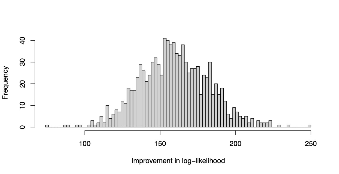
\[T = \log(L_{\tt GLMNET}) - \log(L_{\tt HDGB2})\]

is recorded for each replicate. The simulation is repeated for 1,000 replications, and the resulting \(T\) values are plotted as a histogram. The result is shown in Figure 2. The reader may verify that the log likelihood clearly improves with the HDGB2 routine. The reason is because the true underlying distribution is GB2, and HDGB2 results in a better fit in the out-of-sample. This demonstrates the advantage of HDGB2. It should be made clear that the study does not claim that the prediction results are necessarily better in terms of the correlation in the out-of-sample, or in terms of the Gini index as defined in Frees, Meyers, and Cummings (2011). What this shows is that the distribution may fit the true distribution better in terms of the log likelihood if the true underlying distribution is in fact GB2 instead of log-normal. This yet is an achievement to be excited about, because the HDGB2 allows for shrinkage and selection of the explanatory variables and yet provides a GB2 distribution fit.

5. Real data study

In this section, the results of a real data study will be demonstrated. The real data analysis has been performed on the crop insurance indemnities data, available from the USDA Risk Management Agency (RMA) website: https://www.rma.usda.gov. The goal of the analysis is to predict crop insurance indemnity amounts using a set of explanatory variables, including the log-liability amounts of each farm, the type of crop grown at the farm, and the county code of the farm. The idea here is that using regression shrinkage and selection methods, we may avoid overfitting of the model and improve the fit of the loss model. Summary statistics for the exposure variable, and the response in the training sample are shown in Table 1.

The summary statistics in Table 1 are computed using a sample of size 1,934. This sample has been obtained by taking a subset of the full crop insurance dataset from 2019, selecting those observations with positive liability and indemnity amounts within the state of Michigan, and finally selecting a training sample by randomly choosing 50% of the observations. Notice that the liability amounts and indemnity amounts are all positive. The remaining 50% of the observations within Michigan are used for validation. Table 2 shows the indicator variables used for the regression analysis, along with their means.

In Table 2, the first set of variables are indicators of specific counties within Michigan. The second set of variables are indicators for specific commodities within Michigan. For example, the variable Soybeans is an indicator for whether the observation is for a farm that grows soybeans. The table shows that 30.6% of the farms are growing soybeans within Michigan. Likewise, about 2% of the farms are growing cherries. The design matrix \(\mathbf{X}\) is constructed using the log liability exposure variable, and the indicator variables summarized in Table 2. The HDGB2 routine, and the log-normal GLMNET routine are used to regress the response on the explanatory variables, with shrinkage and selection. The resulting coefficient estimates are shown in Table 3.

Table 3 shows that the two routines resulted in roughly similar coefficients for the exposure variable, and resulted in a different set of non-zero coefficients. Yet, Ionia and Sanilac both resulted in zero coefficients for both of the models. Also, dry beans, potatoes, and grapes resulted in zero coefficients for both of the routines.

In Figure 3, the reader may observe that the coefficients for each variable are shrunk towards zero, as the tuning parameter \(\lambda\) is increased. In the left panel of the figure, the result from a ten-fold cross validation is shown with the tuning parameter value that minimizes the log score indicated with a vertical line. The right hand panel shows the solution path, as the tuning parameter is decreased from the maximum possible value to the optimal one indicated by the vertical line on the left panel.

Looking at Table 4, the full GB2 regression, which uses the full set of explanatory variables, plus three shape parameters, and an intercept, results in a 74.0% out-of-sample Pearson correlation with the actual indemnities, and a 70.1% Spearman correlation. When the prediction is performed using a lasso approach with a log-normal assumption of the indemnities, using the GLMNET R package, it results in a 52.8% Pearson correlation in the out-of-sample, and a 74.0% Spearman correlation. Our proposed approach, using a GB2 model with regression shrinkage and selection resulted in a 85.5% out-of-sample Pearson correlation, and a 72.9% Spearman correlation. Presumably, the GB2 model with regression selection has improved the performance of GLMNET in terms of Pearson correlation by imposing the correct distributional assumption on the response.

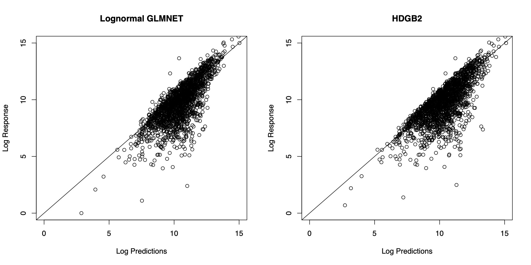
In Figure 4, the prediction results from the two models are compared. In order to generate predictions from the model estimated by HDGB2, note that the GB2 distribution may not have finite moments. For this reason, the predictions are generated by taking a specific quantile of the distribution, where the quantile is determined by finding the value that minimizes the squared difference between the prediction and the response within the training sample. The figure shows that the two models fare about the same in terms of the prediction result. The correlation with the out-of-sample indemnity amounts for each of the model is summarized in Table 4. It must be emphasized that the goal of HDGB2 is to improve the distribution fit, while still allowing for variable selection, more so than necessarily improving the prediction result from a log-normal GLMNET.

The resulting set of shape parameters and regression coefficients are used to obtain a QQ-plot to determine how good the fit is. Figure 5 shows that the fit of the HDGB2 routine is better than when a log-normal assumption is used with the GLMNET package. This is the main result of the paper. Although the results for the out-of-sample prediction are somewhat mixed, the message in Figure 5 is pretty clear: HDGB2 results in a better fit, especially in the tail parts of the distribution, when the underlying loss distribution has heavy skewness. A better distributional fit may be beneficial in applications where the theoretical percentiles of the outcomes are needed, such as excess layer pricing, or reserving problems.

6. Conclusion

This paper introduces an approach to incorporate variable shrinkage and selection into models commonly used in actuarial science. We have applied the approach to the Burr distribution for illustration, and the GB2 distribution. For the GB2 distribution, the paper describes in detail the implementation of the HDGB2 regression routine, allowing for automatic shape parameter estimation and regression shrinkage and selection with cross validation. The resulting routine has comparable variable selection capabilities with the GLMNET routine, although the resulting set of variables corresponding to non-zero coefficients may be different. The prediction result is roughly similar to the log-normal GLMNET approach. The main advantage of the HDGB2 routine is that it results in a better fit of the distribution, when the underlying true distribution of the data is indeed GB2. We have demonstrated that the fit results in a better QQ-plot in case of the U.S. crop insurance data (for the Michigan subset) obtained from the RMA.

We conclude the paper with some honest discussion of the limitations of the model. We have implemented the shrinkage and selection routine for the GB2 severity model, but have not done so for the frequency distribution. The purpose of the paper is to illustrate the shrinkage and selection approach for one of the most widely used distributions in research nowadays, more so that demonstrating it for all of the various distributions known in actuarial science. It may be interesting future work to apply the method to frequency distributions, and more severity distributions not discussed in this paper. The goal of this paper is to motivate such potential future work, and illustrate the viability of shrinkage and selection estimation within actuarial science.

---

Acknowledgement

This research has been generously funded by the Casualty Actuarial Society (CAS) via the 2020 CKER/CAS Individual Grant Competition. The author would like to thank the CAS for making this work possible. The author would also like to thank the editor and two anonymous reviewers, who provided constructive comments to improve the quality of this paper.