1. Introduction
Recommender systems (RSs) are machine learning algorithms that suggest to loyal clients the best next product to buy or propose to prospective customers the most appropriate set of products (Ricci et al. 2011).
Currently, these algorithms constitute one of the more active research areas of machine learning (ML), partly because of their successful employment in various business sectors, from the entertainment industry to e-commerce. Netflix’s movie suggestions (Netflix 2009), Amazon’s recommended site sections, and Twitter’s “users to follow” are just a few well-known outstanding examples of RS use cases.
However, despite this great popularity, the insurance industry (II) has paid relatively little attention to them. In particular, by mid-2018 only a few articles (Mitra, Chaudhari, and Patwardhan 2014; Rokach et al. 2013; Qazi et al. 2017) in the actuarial literature had focused on the application of RSs to the II. The reasons behind the paucity of scientific papers have mainly to do with the intrinsic nature of the II when compared to other fields, where RSs have been rewardingly applied (Rokach et al. 2013). Building an RS capable of bringing value to both companies and consumers, using canonical techniques, requires either a large set of similar products to recommend or a vast amount of unwittingly provided profiling data characterizing clients and prospects. In contrast, in the insurance industry the number of products available is relatively small, limiting the effectiveness of classical RS models. Moreover, many techniques adopted in RS analyses are quite different from those routinely used by actuaries. Nevertheless, we believe that unlocking the potential of RSs in the II could probably benefit insurers—that is, by proposing the purchase of nonregulated coverages, which typically offer a higher underwriting margin than regulated ones.
This work aims at providing an overview of the state-of-the-art RS algorithms from theory to code implementation in a real-case scenario, showing that such techniques could find fruitful application in actuarial science. Furthermore, we suggest a way to mathematically model the recommendations in the II field and we build an RS approach based on supervised learning algorithms. For our data, this suggested method shows promising results in overcoming the difficulties of the classical RS models in the II.
2. Brief literature review
According to Sarwar et al. (2001), RSs consist of the application of statistical and knowledge discovery techniques to the problem of making product recommendations based on previously recorded data. The objective of making such recommendations is the development of a value-added relationship between the seller and the consumer, by promoting cross-selling and conversion rates.
RSs date back to the early '90s with the Apriori algorithm (Agrawal and Srikant 1994). Basically, this technique returns a set of “if-then” rules that suggests the next purchase given the history of previous transactions (“market basket”) using simple probability rules. Nowadays, RSs are grouped into two macro categories: those using “collaborative filtering” (CF) reasoning and those using “content-based filtering” (CBF) (Ansari, Essegaier, and Kohli 2000). Whereas the CF approach computes its predictions on the behavior of similar customers (Breese, Heckerman, and Kadie 1998), the CBF approach uses descriptions of both items and clients (or prospects) to understand the kinds of items a person likes (Aggarwal 2016). For an exhaustive discussion, Ricci et al. (2011) provide a broad overview.
As one may note from the increasing relevance of the RecSys conference (Association for Computing Machinery 2018), literature regarding RSs is vast and growing. Nevertheless, it is a topic little explored in actuarial and insurance-related research. In Mitra, Chaudhari, and Patwardhan (2014), we found an analysis of the potential of RSs in the II, but mostly from a business perspective and without an empirical approach. On the contrary, Rokach et al. (2013) underscore the difficulty of applying RSs in the II, addressing the issue of the small number of items to recommend. Nevertheless, the paper showed that adopting a simple CF algorithm to recommend riders could significantly benefit sales department productivity.
Qazi proposes the use of Bayesian networks to predict upselling and downselling (Qazi et al. 2017); however, the paper provides scarce details of the methodology.
It is important to stress that none of the techniques discussed in Mitra, Chaudhari, and Patwardhan (2014), Rokach et al. (2013), and Qazi et al. (2017) belongs to any model class with which actuaries would be familiar. For that reason, we offer an overview of the classical RS algorithms in the following sections.
3. The framework
In this section we introduce how to build and evaluate a model based on machine learning algorithms, focusing our attention on the development of a recommendation system for insurance marketing. In particular, we stress that our final goal is the construction of an RS that can predict a client’s propensity to buy an insurance coverage in order to support business decisions.
3.1. Methodology
3.1.1. Modeling ratings data
Most classical RSs base their suggestions on a ratings matrix that encodes information about customers and products. The name “ratings matrix” comes from the fact that originally each row contained customer ratings for sold products. In practice, the element could be expressed in either a numeric-ordinal scale (for example, one-to-five-star rating) or using 0–1 data, sometimes referred to as “implicit rating” (IR). In other words, IR represents data gathered from user behavior where no rating has been assigned.
IR is the data format most relevant for our application: a value of 1 means that the policyholder has expressed a preference for (i.e., purchased) that specific insurance coverage, while a zero value can mean that the customer does not like the product, does not need it now, or is unaware of it. Thus, while the 1 class contains only positive samples, the zero class is a mixture of both positive and negative samples. In fact, it is not known whether the policyholder dislikes the item or would appreciate it, if he or she were aware of it. For the sake of completeness, other forms of IRs can be represented by the number of times the user purchased that specific product or by the times that product has been used (in the entertainment industry, for example).
A frequently used metric to compute product similarities in the implicit data context is the Jaccard index (Jaccard 1901), with representing the number of occurrences where products A and B are jointly held.
ML predictive algorithms are usually identified by a family of models. Such algorithms typically depend on the choice of one or more hyperparameters, within specific ranges, whose optimal value cannot usually be known a priori. The process of determining the best set of hyperparameters, known as “model tuning,” requires the testing of the algorithm over different choices of hyperparameters. This procedure is a fundamental step for the success of most ML models.
The simplest approach to this problem consists of the adoption of a Cartesian grid to sample over the hyperparameter space. Because this issue is crucial and deserves much thought, we address the interested reader to the work of Claesen and Moor (2015) for more refined techniques.
3.1.2. Assessing performance
An important consideration is the assessment of model performance. In particular, we need to understand how good a developed model is and how to compare alternative models.
Typically, the performance of a model is evaluated on a holdout data set, e.g., splitting customer data (usually the data set rows) into training and testing groups, or using a more computationally intensive k-fold cross-validation approach, which is a standard in predictive modeling (Kuhn and Johnson 2013).
When dealing with RS data, Hahsler (2018) suggests the following approach for the test group recommendations: withhold one or more purchases from their profiles, apply the chosen model, and assess how well the predicted items match those of the withheld ones. For binary and IR data, this reduces to verifying that the withheld items are contained within the top-N predicted items.
When ratings are produced for implicit data, binary classification accuracy metrics (like accuracy, AUC, log loss, and so forth) can be used to score and rank RS algorithms. In particular, the log loss metric measures the discrepancy between estimated and actual probabilities of a target i-th event occurrence, :
logloss=−1nn∑i=1[yi⋅loge(^yi)+(1−yi)⋅loge(1−^yi)].
On the other hand, the area under the receiver operating characteristic (ROC) curve (known as the AUC) measures the model’s ability to classify the target (binary) outcomes. In fact, a model’s output can be used in a decision-making process, defining a certain threshold and classifying cases as belonging either to the purchaser category or not whereby their score is higher than the set threshold. It is possible to cross-tabulate actual and predicted groups using something known as the “confusion matrix,” which can be synthetized as follows, where is the total scored sample size:
| Predicted | Observed: Event | Observer: Non-Event |
| Event | True Positive (TP) | False Positive (FP) |
| Non-Event | False Negative (FN) | True Negative (TN) |
Performance metrics such as the following can be created on such a matrix:
- Accuracy,
- Sensitivity (recall),
- Precision (positive predictive value),
- Specificity (true negative rate),
- Negative predictive value,
As Kuhn and Johnson (2013, 262-65) well detail, these metrics depend on the selected threshold value; in particular, there is a trade-off between sensitivity and specificity, and the AUC represents the area under all possible combinations of sensitivity and specificity as a function of the selected threshold.
Briefly, the log loss metric is used when it is necessary to estimate the probability as precisely as possible, while the AUC score is more appropriate when it is more important to distinguish between two classes (such as purchasers and non-purchasers for marketing strategy).
Furthermore, if two periods of data are available, a possible strategy is to build the RS based on the initial-period data in the training set and to assess how well the algorithm predicts purchases in the next period in the test set. This work adopts this assessment approach. We remark that the scoring is clearly performed on a product basis and is evaluated only on customers that do not hold that precise product in the initial period.
We stress that although splitting the data set into the training set and the test set is not necessary for all the approaches presented in this paper, for the sake of comparison of the algorithms, it has been shared across all the techniques.
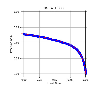
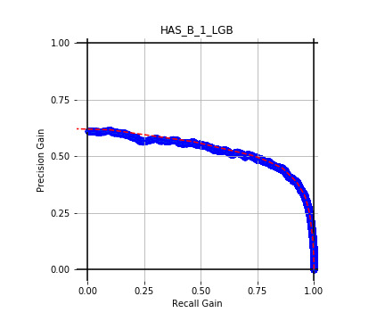
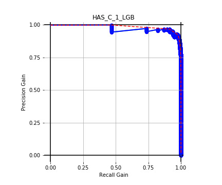
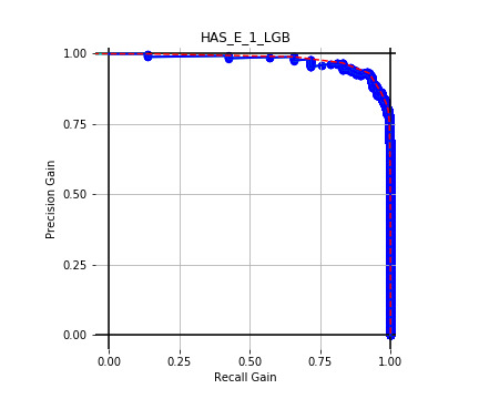
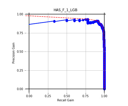
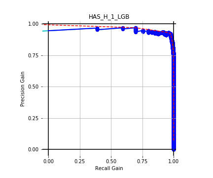
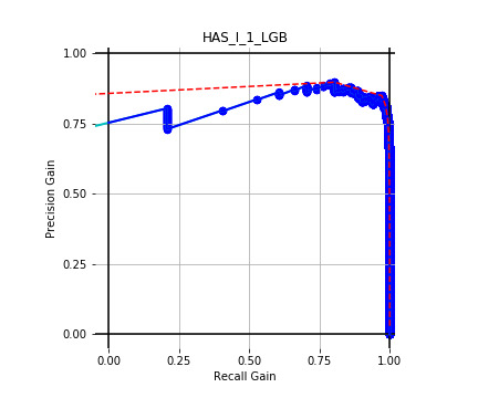
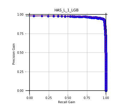
We decided to use the ROC AUC as the metric to test the algorithms because of its ability as a ranking performance measure (Flach and Kull 2015; Hand and Till 2001). Our recommendation approach is not based on a classification task (i.e., client A is going to buy a specific product or not) but rather on a ranking task (i.e., client A is more inclined to buy a specific product than client B).
For that reason, we prefer the ROC AUC, although our data set presented highly unbalanced classes, as usually happens for some kinds of insurance coverages. The appendix briefly addresses this specific issue.
3.2. The available data and modeling limitations
The chosen algorithms will be trained on an anonymized insurance marketing data set containing about 1 million policyholders’ purchased coverages in two subsequent periods, as well as some demographic covariates. The examined approach’s ability to predict next-period purchases (from the set of insurance coverages still not held) is measured. Supplementary binary variables indicate whether the policyholder purchased the coverage in period one and whether the policyholder purchased the coverage in period two; we use this supplementary information to assess the performance of the analyzed RSs.
We exclude CBF algorithms from our analysis, because the number of possible kinds of insurance coverage is lower by an order of magnitude than the number of items typically traded in online industries (e.g., Netflix, Amazon, Spotify, etc.). In fact, our application deals with a small number of products—the different kinds of insurance coverages—that show relative heterogeneity of characteristics. For example, a life or health policy is quite different from auto coverage. For this reason, if one client has both kinds of policies, while another one has just a life policy, the implication that the latter might also like an auto policy does not necessarily hold as easily as it might in other industries where the variety of products is much greater.
In addition, only two periods’ worth of portfolio composition, rather than the full history of previous purchases, is available. For that reason, sequence-based algorithms, which have been found to be extremely useful in the literature, are not considered in this study.
3.3. Mathematical formulation
With regard to the issue of recommendations in the insurance field, we present a mathematical framework capable of describing the functional setting between customers and products. We assume that the willingness of a person to buy a product may be represented by a probability density function depending on the demographic characteristics of the person the social pressure and the timing
It is reasonable to endow the aforementioned variables with the following characteristics:
- The demographic features (i.e., age, gender, wealth) identify the client’s state and account for most of the value.
- Strong social pressure might increase (or decrease) the likelihood of buying a product —hence can be regarded as a quantity that explains factors external to the client (i.e., advertisement campaigns or client networks).
- The timing is a random variable that models phenomena related to unpredictable events (e.g., a tennis player who loses his racket might need a new one)—thus, this variable is usually not detectable.
In an RS framework, typically product similarity bias is also often taken into account. However, as pointed out previously, in the insurance market the number of diverse products is small, and hence this bias effect, if present, can be neglected. For this reason, the initial assumption of a probability function dependent only on a single product rather than the entire set of products could be reasonable.
Notwithstanding this framework, finding the analytic formulation of the function or discovering the dynamics of the problem is a complex task.
In the latter part of the following section, we propose a way of exploiting supervised learning algorithms for learning the function explicitly based on the client’s demographic features disregarding the timing and the social pressure variables due to the lack of data. In particular, the next section is devoted to the implementation of all the classical RS approaches for the sake of completeness and comparison.
4. Statistical techniques
Herewith we provide an overview of different RS algorithms. In particular, we underscore that the power of these techniques lies in their generality. In fact, some of the algorithms presented have been and would be employed to tackle other problems of the actuarial sciences.
4.1. arules
Association rules (arules) is a well-established approach to finding interesting relationships in large databases (Agrawal and Srikant 1994). Following the notation of Hahsler, Grün, and Hornik (2005), let be a set of n binary attributes called items. Let be a set of transactions called the database. Each transaction in has a unique transaction ID and contains a subset of the items in I. A rule is defined as an implication of the form where and The sets of items (for short item sets) and are called antecedent (left-hand-side or LHS) and consequent (right-hand-side or RHS) of the rule. Various measures of significance have been defined on rules, the most important of which are these:
- support, is defined as the proportion of transactions in the data set that contain that specific item set;
- confidence is the probability of finding the RHS given that the transaction contains the LHS: and
- lift is a measure of association strength, in terms of departure from independence:
The process of identifying rules can yield many of them, and thus we usually set a minimum constraint either on confidence or on support, or on both, in order to select “meaningful” rules. In addition, rules are often ranked according to the lift metrics to highlight more important associations. Nevertheless, the selection of the confidence and support thresholds is subjective given that no optimal metric was defined in the original arules model. The interested reader can consult Tan, Kumar, and Srivastava (2004) for a deeper discussion of the topic.
The two most used algorithms to mine frequent item sets are arules and Eclat, with the latter the less well known; Borgelt (2003) provides the interested reader more details about their actual implementation. The arules algorithm has also been extended to work on supervised learning problems, as Hahsler (2018) discuss.
A great advantage of the arules approach is that it provides easily interpretable model output that can be easily communicated to nontechnical audiences, like senior management or producers, in the form of simple directives. A drawback of this technique is that there does not exist a direct measure of predictive performance, especially on one-class data.
4.2. User-based and item-based collaborative filtering
User-based collaborative filtering (UBCF) provides recommendations for a generic user, identifying the users most similar to and averaging their ratings for the items not present in the profile. It is assumed that because users with similar preferences would rate items similarly, missing ratings can be obtained by first finding a neighborhood of similar users and then aggregating their ratings to form a prediction (Hahsler 2018). A common measure of user similarity, at least for non-implicit data, is the cosine similarity (CS) coefficient,
sx,y=→x∗→y∥x∥∗∥y∥,
which, clearly, is calculated only on the dimensions (items) that both users rated. For a given user it is possible to define a neighborhood selecting, for example, the nearest neighbors by CS or another (dis)similarity metric. Then the estimated rating of the th item for the user is simply where each ith neighbor rating has been weighted by its similarity with user A serious drawback of UBCF is that it requires holding in memory the users’ similarity matrix. This makes UBCF unfeasible on real data sets.
Another approach, item-based collaborative filtering (IBCF), calculates similarities within the items’ distances set, whose dimensionality is usually orders of magnitude lower than the users’ one. Then, given similarities between ith and jth items and the neighborhood of the items most similar to the ith, it is possible to estimate As described further, this paper applies IBCF using the Jaccard index as a measure of products’ distances. In fact, the CS coefficient is not suitable when only implicit data are available at the user level, as the jointly purchased products will just be flagged with ones. In general, the Jaccard index appears to be more frequently used when binary or implicit data are used.
Whereas UBCF requires a -sized similarity matrix to be kept in memory, IBCF requires an -sized one; an additional memory reduction is obtained by keeping in memory only the most similar distances. Nevertheless, when the magnitude of the customers’ size is relevant, only IBCF is used, and, empirically, it appears that moving from UBCF to IBCF leads to only small performance losses according to Hahsler (2018).
4.3. Matrix factorization approaches
Matrix factorization techniques, such as nonnegative matrix factorization and singular value decomposition (SVD), are the mathematical foundation of many RSs belonging to the CF family (Koren, Bell, and Volinsky 2009). The matrix factorization approach approximates the whole ranking matrix into a smaller representation:
Rm×n≈Xm×k∗Yk×n.
This artifact both reduces the problem’s dimensionality and increases the computational efficiency. has the same number of rows as the matrix, but typically a much smaller number of columns, is a matrix that represents the archetypal features set generated by combining columns from while represents the projection of original users on the space. The result is twofold: first, each product is mapped on a reduced space representing its key dimension (archetypes); second, it is possible to compute products-dimension preferences for each given customer. For example, if we think of products as a combination of a few “essential” tastes, the matrix represents all items projected in the taste dimension, while the matrix presents the projection of all users in the taste dimension. Therefore, the rating given by subject to product is estimated by Our analysis considers four algorithms in this category that represent different variations of the matrix decomposition approach —LIBFM, GLRM, ALS, and SLIM.
4.3.1. LIBFM
A typical solution for and can be found solving
minX,Y(∑(u,v)∈R[f(xu,yv;ru,v)+μX||xu||1+μY||yv||1+λX2||xu||22+λY2||yv||22]
as shown in Chin et al. (2015), where is the loss function and are penalty coefficients similar to the ridge and lasso ones of the elastic net regression model (Zou and Hastie 2005). For binary matrices, the logarithmic loss is typically used as well as binary matrix factorization (Z. Zhang et al. 2007). This algorithm is efficiently implemented in the LIBFM open-source library, from which it takes its name (Chin et al. 2016).
4.3.2. GLRM
Udell et al. (2016) recently introduced the generalized low rank model (GLRM) approach, which is another approach to effectively perform matrix factorization and dimensionality reduction. The compelling feature of this approach is that it can handle mixed-type data matrices, which means that the GLRM can handle matrices filled not only with numerical data but also with some columns of categorical, ordinal, binary, or count data. This is achieved by imposing not just a single loss function but many according to the category of the columns. This enables the GLRM to encompass and generalize many well-known matrix decomposition methods, such as PCA, robust PCA, binary PCA, SVD, nonnegative matrix factorization, and so on. As for LIBFM, the GLRM approach supports regularization, thus allowing the estimation process to encourage some structure such as sparsity and nonnegativity in and matrices. Notable applications for GLRMs lie in missing values imputation, features embedding, and dimensionality reduction using latent variables.
4.3.3. ALS
The Alternating Least Squares (ALS) algorithm (Hu, Volinsky, and Koren 2008) was specifically developed for IR data. Used by Facebook, Spotify, and others, it has gained increasing popularity. That Apache Spark, a well-known open-source big-data environment, chose to implement ALS as the reference recommendation algorithm (Meng et al. 2016) for its machine learning engine (Mllib) confirms its importance. Like the previously mentioned ML methods, the ALS algorithm aims to decompose the rating matrix, and are initially randomly populated, and then least squares minimization is used in an iterative manner to obtain their optimal values. “Alternating” means that each loss minimization iteration comprises two steps: in the first, is fixed and is optimized, and in the second, the reverse happens. ALS is specifically suited for IR, since it introduces the concepts of manifest “preference” and confidence which is a measure of how explicit ratings reflect a true preference. Formulaically,
p_{{ui}} = \left\{ \begin{matrix} 1 & r_{{ui}} > 0 \\ 0 & r_{{ui}} = 0 \\ \end{matrix} \right.\ \ ,
and, for confidence
c_{{ui}} = 1 + \alpha*r_{{ui}}.
This means that a minimal confidence exists even if the user has never purchased the product and that increasing interactions between the user and the product linearly increase the confidence. Hu, Volinsky, and Koren (2008) suggest values between 15 and 40 for in their application. Clearly, when only single-purchase data (as in our insurance application) are available, confidence is of limited use, but it could be more useful in cases where several periods’ worth of renewal history is available.
The loss function to be minimized becomes
\underset{x^{*},y^{*}}{{\min}}\sum_{u,i}^{\mathstrut}c_{{ui}}\left( p_{{ui}} - x_{u}^{T}y_{i} \right)^{2} + \lambda\left( \sum_{u}^{\mathstrut} \mid x_{u}\overset{2}{\mid} + \sum_{i}^{\mathstrut} \mid y_{i}\overset{2}{\mid} \right),
from which, after some algebra, the following alternating equations can be found:
\left\{ \begin{matrix} x_{u} = (Y^{T}Y + Y^{T}*\left( C^{U} - I)Y + {λI} \right)^{- 1}Y^{T}C^{u}p(u) \\ y_{i} = (X^{T}X + X^{T}*\left( C^{i} - I)X + {λI} \right)^{- 1}X^{T}C^{i}p(i) \\ \end{matrix} \right.,
where is the identity matrix, and are initially randomly filled, and, as for many of the other methods herewith presented, represents a penalty constant (usually set between 0.1 and 0.01). The similarity between item and other items can be found by the following matrix operation: as well, recommendations for user and each item are derived by
4.3.4. SLIM
The sparse linear method (SLIM) algorithm, as presented in Ning and Karypis (2011), blends ideas from matrix factorization and the robust linear model (as the elastic net regression). The recommendation score for the non-purchased item for user is given by where and is a sparse-size column vector of aggregation coefficients. Thus, the SLIM model recommendation scores can be written in the following factorization form:
\widetilde{A} = {AW},
where is the binary user–item purchase matrix and is the matrix of aggregation coefficients. In particular, the column of stands for and and represent the row vectors for the recommendation and purchase histories of user respectively.
The matrix solves the following regularized minimization optimization problem:
\begin{matrix} \underset{W}{\min}\frac{1}{2}\left. \parallel A - {AW} \right.\parallel_{F} + \frac{\beta}{2}\left. \parallel W \right.\parallel_{F}^{2} + \lambda\left. \parallel W \right.\parallel_{1} \\ W \geq 0 \\ {diag}(W) = 0 \\ \end{matrix},
where is the Frobenius norm, and and are the regularization parameters for an elastic net regression, respectively. The nonnegative constraint is applied on such that the learned matrix represents positive relations between items, if any. Imposing a null diagonal for avoids trivial solutions (e.g., the identification of a matrix where an item always recommends itself) and ensures that is not used to compute
It turns out that the columns of the matrix are independent and this makes the computations easily parallelizable. Therefore, the SLIM algorithm efficiently scales on high-dimensional problems. The aforementioned paper shows an empirical analysis applying different CF algorithms on data sets frequently used to benchmark RSs, indicating that the SLIM algorithm often outperforms competing algorithms.
4.4. Supervised learning algorithms
Supervised learning (SL) techniques combine statistical inferential reasoning and approximation theory to estimate an unknown functional relation between two spaces and (Hastie, Tibshirani, and Friedman 2009), respectively denoted as the features space and the predictions space, once provided a set of sample points, called the training set.
\mathcal{S}_{\text{train}} = {\{(\mathbf{x}_{i},\mathbf{y}_{i})\}}_{i = 1}^{N} \subset \mathbf{X} \times \mathbf{Y}
Canonically, the values of the elements in are named predictors and the ones in are called labels. These algorithms, when properly configured, are capable of extracting patterns and correlations, constituted by a mapping
\widehat{f}:\mathbf{X} \rightarrow \mathbf{Y}\quad|\quad\widehat{f} \approx F
which generalizes over previously unseen samples, the testing set:
\mathcal{S}_{\text{test}} = {\{(\mathbf{x}_{i},\mathbf{y}_{i})\}}_{i = 1}^{M} \subset \mathbf{X} \times \mathbf{Y}\quad|\quad\mathcal{S}_{\text{test}} \cap \mathcal{S}_{\text{train}} = \varnothing
meaning that
\widehat{f}\left( \mathbf{x} \right) \approx \mathbf{y}\quad\forall\mspace{6mu}\left( \mathbf{x},\mathbf{y} \right) \in \mathcal{S}_{\text{test}}{\ .}
The function is typically found by solving the following constrained optimization problem through a gradient descent method:
\underset{f}{\text{argmin}}\mspace{6mu} E_{\mathbf{y}}\lbrack l(\mathbf{y},f(\mathbf{x}))|\mspace{6mu}\mathbf{x}\rbrack,\quad(\mathbf{x},\mathbf{y}) \in \mathcal{S}_{\text{train}}
\begin{align} E_{\mathbf{y}}\lbrack l(\mathbf{y},f(\mathbf{x}))|\mspace{6mu}\mathbf{x}\rbrack \approx E_{\bar{\mathbf{y}}}\lbrack l(\bar{\mathbf{y}},f(\bar{\mathbf{x}}))|\mspace{6mu}\bar{\mathbf{x}}\rbrack, \\ (\mathbf{x},\mathbf{y}) \in \mathcal{S}_{\text{train}} \land (\bar{\mathbf{x}},\bar{\mathbf{y}}) \in \mathcal{S}_{\text{test}}. \end{align}
In brief, supervised learning algorithms allow the construction of statistically solid forecasting models based on a given set of observations and associated outcomes. Linear regression is the simplest example of a supervised learning algorithm. But many other approaches familiar to actuaries—such as generalized linear models, or GLMs (McCullagh and Nelder 1989)—belong to the supervised learning class of ML algorithms.
These techniques are increasingly becoming a convenient and essential tool in the actuarial sciences: see, for example, Yang, Qian, and Zou (2018) for the adoption of ML in pure premium estimation; Spedicato, Dutang, and Petrini (2018) for an application in retention and conversion modeling; and the monographs of Frees, Derrig, and Meyers (2014, 2016) for a general overview. In our application, may represent the customer’s demographic profile and the probability of a product’s purchase. A key advantage of an SL approach compared with a CF approach is that it can be fit without any need of the history of previous purchases. Thus, it can provide recommendations not only to existing customers but also to prospective ones. Even if it is possible to use both demographic variables and the history of previous purchases in the SL approach, we choose not to do that in this application.
In what follows we give an overview of some of the more relevant supervised learning algorithms: gradient boosting trees (GBTs) and deep neural networks (DNNs). Although these ML models have usually been regarded as black boxes, research has been devoted to efforts to ease results explainability. In particular, we stress that algorithms exist capable of approximately measuring the marginal effect of single variables over the model’s output and of investigating the overall variable importance. The interested reader is referred to Lundberg and Lee’s (2017) seminal paper and to the DALEX and LIME libraries (Biecek 2018; Pedersen and Benesty 2018).
4.4.1. Generalized linear models
Generalized linear models, or GLMs, represent a class of SL algorithms whose key assumptions are as follows: the observation of the dependent variable belongs to the exponential family with mean and dispersion parameters and respectively; the expected value and variance of are, respectively, and where is a linear (or at least a linear combination of nonlinear terms) and a monotone transformation, which is called “link function”. Some link functions relevant for actuarial science applications are the logarithmic and the logit (i.e.,
Compared to many more recent ML algorithms, GLMs are easily estimated with most open source and corporate software tools (using the maximum likelihood approach). Another important feature is their inherent linearity, which strongly helps to explain modeling results. On the other hand, GLMs do not allow the full modeling of intrinsically nonlinear relationships and they have no mechanism for discarding irrelevant predictors (feature selection) or for self-identifying significant interactions between predictors. Nevertheless, it is possible to fit GLMs using the elastic net approach instead of classical maximum likelihood, which helps to discard non-significant predictors and to make coefficients’ estimates more stable. In addition, common approaches practitioners use to overcome nonlinearity are to transform continuous predictors into categorical ones (e.g., by binning into equal exposure groups, or decile binning) or to use nonlinear additive terms, such as polynomials or splines.
GLMs are the predictive models on which modern insurance pricing is founded, as is detailed in Goldburd, Khare, and Tevet (2016). For 20 years, loglinear Poisson and gamma models have been applied to model claims frequency and severity, while logistic regression has been used to estimate the retention and conversion probability of current and prospective policyholders as a function of rating factors. And a logistic regression would be a proper choice from within the GLM family to model product possession or propensity to purchase insurance coverages.
4.4.2. Gradient boosting trees
Gradient boosting tree (GBT) algorithms are based on an approximation technique, called boosting, that assumes that the function can be approximated as a sum of a finite set of functions being the named “weak-learners”:
b_{i} \equiv b(\mathbf{p}_{\mathbf{i}}):\mathbf{X} \rightarrow \mathbf{Y}{\quad\quad}\forall{\;i} = 1,\ldots N
depending on a set of parameters With these assumptions, the optimization problem introduced at the beginning of this section is transformed into a search for the optimal set of parameters characterizing the boosters and minimizing the expected loss function over the training set, with the aforementioned generalization constraints.
From a computational point of view, the minimum is obtained via a gradient descent method constrained to the booster function at each iteration the so-called stagewise approach (Friedman 2000). In other words, at each step of the optimization procedure, the optimal set of parameters approximating is sampled from the parameters space determining the weak learner
In GBT algorithms, the boosters are represented by shallow regression trees and, therefore, the parameters are given by the ones characterizing the tree itself, such as the tree’s depth or the number of leaves.
Regarding this issue, we decided to test three different implementations of GBT algorithms—XGBoost (Chen and Guestrin 2016), lightGBM (Ke et al. 2017), and CatBoost (Prokhorenkova et al. 2018)—in order to compare their performances. The name XGBoost stands for eXtreme Gradient BOOSTing. It was the first GBT implementation to significantly improve the time of performance, making possible the adoption of GBTs in a wide range of complex and data-demanding learning tasks. LightGBM improves the time of performance of XGBoost by adopting a novel numerical method for tree splitting, while CatBoost handles categorical features based on a smart encoding of the levels of categorical variables into numerical mappings.
4.4.3. Deep neural networks
DNN-based models embed the features space into the labels space, throughout the chained application of a sequence of smooth functions, called layers. Each layer is typically constructed by a nonlinear function called an activation function, applied onto a linear combination of the layer inputs :
l:\mathbf{x}_{l} \rightarrow a(\mathbf{w}_{l}\mathbf{x}_{l} + \mathbf{b}_{l}),
where are called the weights of the layer or neurons, and refers to bias. We refer to the way multiple layers are combined to constitute the NN as network architecture
The parameters characterizing the NN, are obtained by solving the supervised learning optimization problem. More specifically, the so-called back propagation procedure is applied to determine the network parameters minimizing the loss function. A more exhaustive introduction to DNNs can be found in Goodfellow, Bengio, and Courville (2016) and a review of DNNs applied to RSs can be found in S. Zhang et al. (2019).
In the last decade, thanks in part to progress made in the construction of CPUs and GPUs, NNs have been exploited in most ML problems due to their ability to spot complex patterns or highly nonlinear correlations by approximating complicated functions. In fact, to some extent, NNs can be regarded as very efficient nonlinear regressor models (Sarle 1994).
Despite the extreme accuracy of their performance, a major drawback of DNN is their “black-box” nature. In fact, it is difficult to explain why the given input properties produce the obtained results.
5. Empirical application
We applied the previously reviewed techniques to a data set consisting of 1 million subjects who were customers for two consecutive years of a European insurance company. We considered the following group of variables for the analysis:
- Active holding of coverage for nine different categories of products: HAS_A, HAS_B, . . ., HAS_I. Coverage possession was measured both in time zero and one.
- Fifteen categorical and 14 numerical features representing the policyholder’s demographic profile measured in the first year only
- The policyholder unique ID
- A supplementary group of variables, BOUGHT_A, BOUGHT_B, . . ., BOUGHT_E, indicating whether the policyholder acquired the product between the first and second year. For example, the conditions to create BOUGHT_E are This set of variables was used as a target outcome to evaluate the predictive performance of the algorithms.
After preprocessing, the data set was split into a training set, accounting for of the data, and a testing set, comprising the remaining 30%. The testing set was used only for the evaluation of the results, and not during the training phase, to avoid any leakage of information. As Kuhn and Johnson (2013) explain, such a procedure is necessary for the proper construction and the consistent evaluation of any predictive model.
Data preprocessing and descriptive statistics were performed using the R and Python programming languages (R Core Team 2017; van Rossum 1995) as well as packages dedicated to implement the specific algorithms, which are specified in the following paragraphs. We also used other libraries for data management, such as the tidyverse (Wickham 2017) package. While in this section we describe the general implementation approaches for each algorithm herewith presented, the reader may find the full computational details in the code hosted in the GitHub repository. In addition, the appendix contains a few random rows of the anonymized data set used in the empirical part of the paper.
5.1. Product possession distribution
Table 1 represents product possession in the initial period.
Table 2 shows the forthcoming-period purchases, on which the recommender systems’ outputs will be assessed. It can be seen that the purchase of an additional policy, for existing customers, is an infrequent event. Depending on the product, it varies from a minimum value of 0.1% to a maximum value of 2.1%. We take into account the low frequency of the target event as we develop the models.
5.2. Arules
We used the R implementation of the Apriori algorithm in the arules library (Hahsler, Grün, and Hornik 2005). As detailed in the source code, the rule mining requires transforming the transaction data set into a sparse matrix format. In order to identify rules, we must set minimum confidence and support in advance. The increase of the values of both parameters restricts the number of candidate rules, reducing the number of retrieved ones. In addition, one must also set the minimum length of rules found when setting the algorithm. As previously discussed, the choice of such values is mostly subjective and depends on the analyst’s preference; because no goodness-of-fit performance is defined, there is no need for hyperparameter optimization in this context. For our analysis, we judgmentally set the rules’ search with the following criteria:
- Minimum rule length: 2
- Minimum support: 1%—that is, both LHS and RHS must exist in the data set in at least 1% of row transactions
- Minimum confidence: 20%, which means that the probability of RHS occurrence, given LHS, should be at least 20%
Only two rules were found. Table 3 shows them, sorted by decreasing lift.
If we add the constraint of positive association (lift greater than one), we are left with only one rule. Basically, that rule says to suggest purchasing B to all customers that have already purchased coverages A and D since this holds for 38% of customers holding products A and D. We tested this rule on policyholders that do not have the B coverage at time zero, and we measured the AUC of predicting actual B purchased in the 0–1 period using the simple rule identified by arules. The AUC is just slightly higher than the noninformative value of 0.5, 0.52 precisely, while the two other binary classification metrics, the true positive rate (also known as sensitivity) and the true negative rate (specificity), are, respectively, 0.12 and 0.92. The low sensitivity indicates a poor ability in detecting customers that are willing to purchase the product.
5.3. Item-based collaborative filtering
We discarded the user-based collaborative filtering (UBCF) approach because it requires the complete between-users distance matrix. This would make the model unfeasible for real business. We use the recommenderlab R package (Hahsler 2018) implementation of the item-based collaborative filtering (IBCF) approach to fit the model. This R package implements many CF algorithms as well as an infrastructure for evaluating RSs for both continuous and binary ratings. For each product, the Jaccard similarity index is calculated with all other distinct products, but only the top are kept. The IBCF approach requires the number to be specified in advance. The CS metric would not be appropriate for binary data, since it must be computed on commonly purchased pairs and the value on the rating matrix would always be one. Taking into account the relatively small number of alternative coverages, we subjectively set equal to two. A few justifications for that choice follow. As with matrix factorization approaches, we wanted to significantly reduce the dimensionality of the problem, and thus the square root of the number of available products would be the upper bound for : In addition, using the two most similar products would make the algorithm easier to communicate to and be accepted by a nontechnical audience. The resulting Jaccard similarity weighting matrix is shown in Table 4.
Matrix non-null entries represent the similarity score (the Jaccard index, between product and values lower than the top ones per row have been zeroed. values are also used as a propensity-to-purchase score for product for users holding product For each user, the products’ propensity scores have been computed as shown in Hahsler (2018, 7). As was done when estimating the arules model, we computed the AUC for purchases of each product k for policyholders not having product beginning at time 0 as shown in Table 5.
5.4. Matrix factorization approaches
In general, based on our judgment, we chose that the dimension of the archetypal space would be between two and three, while the number of columns of the rating matrix—that is, the number of different insurance coverages—would be 10. The following paragraphs set forth the models’ specific implementation details.
5.4.1. LIBFM
We used the R implementation of LIBFM from the recosystem package (Qiu et al. 2017). The package requires that the data be put in long format; thus there is one observation for each rating made by a policyholder. Also, it requires one to specify the actual loss function to minimize (in our case, the choice was obviously log loss) and some tuning parameters: the dimensionality of the matrix factorization in terms of number of latent factors ridge and lasso parameters. As shown below, we can perform a grid search to identify the optimal choice of the tuning parameters:
- matrix dimension: 2 and 3
- loss: (log)loss
- learning rate: 0.05 and 1
- costp_l1, costq_l1: 0.05 and 0
- costp_l2, costq_l2: 0.001 and 0
After retrieval of the optimal configuration of tuning parameters, the optimal parameters can be used to retrieve the final model. Nevertheless, the overall performance of the model is quite poor, as Table 6 shows.
5.4.2. GLRM
We used the R implementation of the generalized low rank model (GLRM) algorithm provided by the H2O platform (LeDell et al. 2018). The H2O software currently supports the top ML suites. H2O efficiently implements most relevant supervised (random forest, deep learning, GLM, GBM, etc.) and unsupervised (K-means, PCA, GLRM) algorithms supporting parallelization, GPU training, and an easy structure to perform hyperparameter optimization and scoring. Fitting the GLRM requires that the input rank matrix be provided to the H2O functions and also that the following (major) parameters be specified:
- the loss functions by columns;
- the rank of the and matrices;
- the type of regularization (ridge, “L1,” or lasso, “L2”) chosen; and
- the regularization weights on and
As for most ML models, the optimal hyperparameter configuration cannot be retrieved analytically and must be found using a grid search approach. A generalized loss (known as the “final objective value”) is defined for the GLRM, and it is possible to identify parameters’ configuration within a grid that minimizes such a search (using, e.g., a random grid search), similar to the LIBFM approach. The H2O documentation suggests to randomly set missing a percentage of the input matrix entries (e.g., 20%) and to evaluate the ability of the matrix decomposition solution to “reconstruct” the complete matrix (as measured by the final objective value).
After having found the best configuration of parameters, we apply that configuration on our GLRM in order to find the and columns. The reconstructed matrix is then used as scores to identify purchase propensity for each product (by columns). The AUC of GLRM scores on time-one purchases is shown in Table 7.
The AUCs are higher than 0.5 (thus some predictive performance is evident) and in some cases are fairly high (> 0.70).
5.4.3. ALS
To the best of our knowledge, the only efficient implementation of the ALS algorithm without setting up a Spark cluster is the implicit Python package (Frederickson 2018). That library provides an efficient implementation of various implicit rating matrices factorization algorithms. A three-factor solution was fit, leaving the and parameters as default.
The actual predictive performance on the test set was nevertheless negligible, as Table 8 shows.
5.4.4. SLIM
We used the R implementation of the SLIM algorithm in the slimrec package (Srikanth 2017). The estimation procedure is as follows:
- Find the optimal weight between the ridge and lasso regression,
- Estimate given the best alpha on the training set.
- Estimate the recommendation scores,
Table 9 displays the predictive performance of the SLIM model. As the table displays, for some products, it can be relatively high.
A section in the appendix shows the estimated matrix and an example of the calculation of predicted ratings for a customer sample.
5.5. Supervised learning models
5.5.1. Overview
Taking into consideration the available client data and the supervised learning settings, we trained for each policy in our set of coverages the chosen GBT algorithms by providing them the demographic characteristics as inputs once properly preprocessed, and the possessions of a fixed product at time as labels (i.e., is when the client holds the coverage and otherwise). All the algorithms we employ for this analysis minimize the log loss during the training phase, since we want to model a probability. For the NN, we trained only one network for the sake of time constraints; therefore, we adopted the vectors of possession as labels and the categorical cross-entropy as minimizing loss.
The function learned through the prescribed training procedure, provides as output numbers between and is a close approximation of a probability (Kuhn and Johnson 2013), and represent a score of how much a client is inclined to hold the coverage conditioned to the inputs : a numerical representation of the functions introduced in the previous section given the available data.
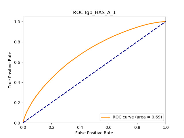
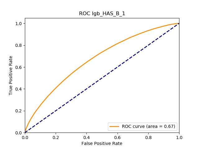
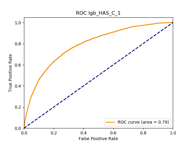
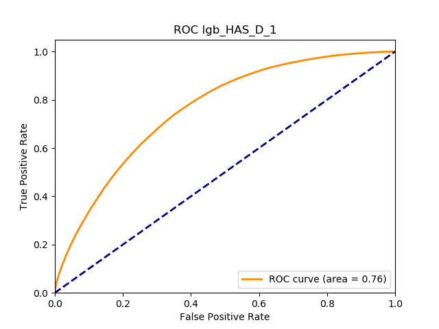
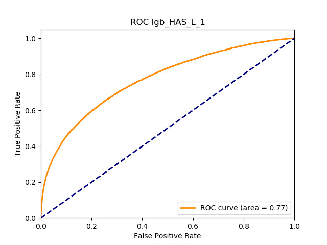
Consistent with what has been done before, the models were constructed using first-period training data and using HAS_X (i.e., possession of product X) as a response variable. Then, predictions have been calculated for test set data. Finally, we calculate the AUC comparing the above predictions to the variable (i.e., the purchase of product X between period one and two) on the test set records that have in the first period.
Recalling our objectives, it is worth noting that when training the algorithms, we are assuming that the propensity of owning a product is shadowing the one of buying that same product. This fact is in contrast with how supervised learning algorithms have been presented in the previous section, the canonical theoretical framework. Here, instead, we are testing the derived models on a response that is different than the one on which they are trained, but related.
As previously shown, the actual period-one purchases are significantly lower than 1% for many products in our data set. Thus, while it was theoretically possible to model directly the one-year probability to purchase, estimated probabilities would be affected by a much higher uncertainty.
5.5.2. Generalized linear models
We used logistic regressions, fitting separate models for possession of each product in the initial period. To handle potential nonlinearities, continuous predictors were transformed into categorical ones using tercile binning (i.e., each new variable has three possible levels that indicate in which tercile the original value lies). Coefficients were estimated using the elastic net approach, performing a grid search over the global penalty weight parameter The R version of the H2O software was used to fit the GLMs.
All of the AUC values are significantly above the noninformative threshold, and many products report an AUC above 0.70 indicating good classification ability, as Table 10 indicates.
5.5.3. Machine learning models: GBT and deep learning
We employed three boosting algorithms: XGBoost, lightGBM, and CatBoost. For all the GBT algorithms we preprocessed the categorical variables in order to group the states accounting for less than the first percentile in a new state, labeled “others.” In more detail, we performed a one-hot encoding on the categorical variables to train XGBoost and a label encoding for lightGBM. We did not need to apply any transformations for CatBoost because it accepts categorical features.
All of these algorithms have different sets of hyperparameters, which were selected through threefold cross-validation, trained over a representative subset of the data. Since the procedure is time-consuming, we tested only a subset of all the possible admissible parameters. Hence, we cannot assure the reader of having found the optimal hyperparameters for our data set, but this was not an issue in this work.
For the deep learning (DL) algorithm, the input data were preprocessed to obtain numerical inputs contained in the interval, which is a requirement of the algorithm. On categorical variables, we applied an entity-embedding layer (Guo and Berkhahn 2016), which encodes categorical features into a -dimensional hypercube where is smaller than the number of the categorical classes. Meanwhile on numerical features, we used a min-max scaling transformation. We adopted Keras with a TensorFlow back-end as a DL framework (Chollet 2017). To construct the presented network, we tested several architectures; however, as with the GBT algorithms, we cannot guarantee that the provided solution is the optimal one.
5.5.4. Results
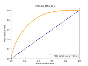
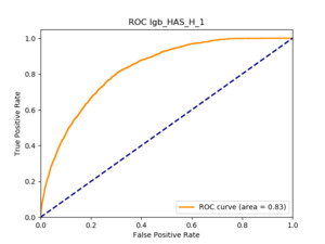
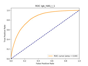
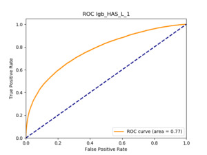
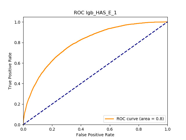
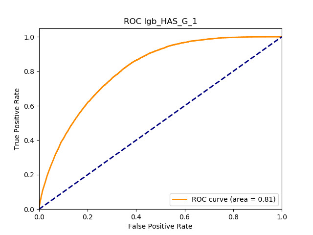
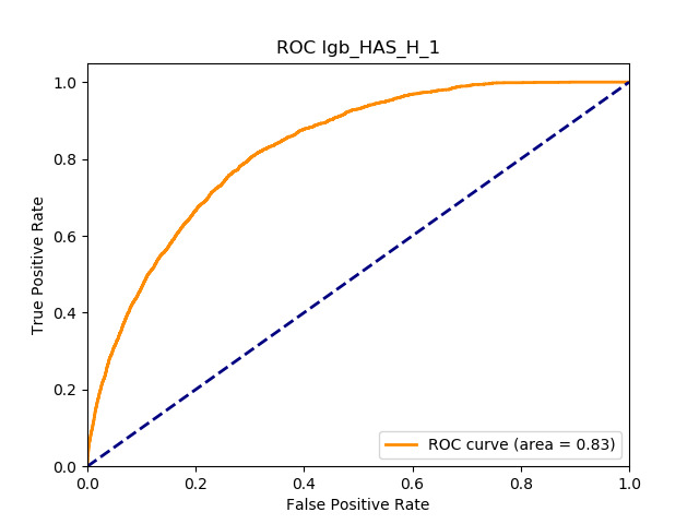
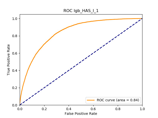
Table 11 displays the AUC values for the supervised learning algorithms. As expected, the predictive performance is always significantly higher compared to the canonical RS approaches, and to the GLMs, even if to a lesser extent. Furthermore, we note that there is no absolute winner among the chosen techniques, since the differences among them are small and could be attributed to suboptimal hyperparameter choices.
6. Summary and concluding remarks
The scarce literature we have reviewed underscores the difficulty of using RSs in the II due to the cardinality of the product portfolio, which is almost always orders of magnitude smaller than in other industries. The small number of products offered might also have an impact on the performance and efficacy of some of the algorithms we discuss. Nevertheless, widespread interest in RSs has arisen in the ML community, and given the role RSs could play in supporting insurance underwriting, we believe actuaries should be aware of such systems’ potential, even if that may be limited compared to their application in the e-commerce and entertainment industries.
We applied common RSs to a real II data set, and that allows us to compare the algorithms in different dimensions: predictive accuracy, easiness of implementation, and interpretability.
In terms of predictive accuracy, what is of most interest to the insurer is a model’s ability to target existing policyholders’ willingness to purchase additional coverage not currently in their portfolio. In this regard, the AUC on forthcoming-period purchases can be thought of as a reasonably accurate metric.
Table 12 reports each RS model’s AUC by product. We see that the ALS and LIBFM algorithms perform poorly on this data set, as their AUCs indicate little if any discriminating ability. On the other hand, the respective performances of the supervised learning methods are very similar and generally good. SLIM offers a good predictive performance, close to the ability of the other supervised learning models. The GLRM matrix decomposition technique displays some discriminating ability, but certainly lower than the above-mentioned models. Finally, the IBCF approach displays a fair discriminating ability, with values that are generally higher than the noninformative value of 0.5. The poor performance of the ALS and LIBFM algorithms could be because of their need for a much larger number of columns in order to work properly. It could be of some interest to confirm such findings using different and possibly wider-ranging insurance-marketing-related data sets.
Calculating the average rank of each RS model (shown in Table 13) provides a quantitative supplement for the analysis. Here, a lower average rank indicates superior predictive performance:
We have omitted the arules model from the analysis since it was not possible to provide rules for all products and since the provided rules offered a predictive performance only slightly above the noninformative value.
While the SL models offer superior performance, they do require much more modeling, data preparation efforts, and computational timing, orders of magnitude higher than what most CF models require. This is especially true for the ML models (deep neural networks and gradient boosting trees), which also almost always suffer from lack of interpretability. They require not only dependent variables (product possession) but also available demographic predictors to be preprocessed. Also many different models must be tested, and all of the presented models involved hyperparameter tuning. IBCF involves that also, but on the other hand, IBCF tuning is generally the fastest among the presented models. It appears that the SLIM model offers a very good balance between computational timing and predictive performance: its average rank score is just below that of the GLMs, without the need for the data preparation and computing time that GLMs require.
It is our impression that only the arules model, and to a lesser extent the IBCF approach, provides a directly intelligible output. In fact, association rules can be expressed in “if-then” rules form, and IBCF is based on an item–item similarity matrix that can somehow be intuitive. The GLMs can still be considered interpretable models, but they could require more effort than the aforementioned approaches. This consideration is valid also for the SLIM approach, where the product suggestions can be seen as a weighted combination of the existing product portfolio. The other models are either different forms of matrix decomposition or nonlinear or tree-based classification models (the SL models), and only recently have tools been developed to improve the methods’ interpretability.
Herein we have explored only a fraction of the methodologies used in the burgeoning field of RSs as at the end of 2018. A broad and practical presentation of many relevant RS algorithms implemented in modern Python software can be found in Javier Rodriguez Zaurin’s GitHub repository (Zaurin 2019).
Acknowledgments
The work was sponsored by the Casualty Actuarial Society (CAS), the Actuarial Foundation’s Research Committee, and the Committee on Knowledge Extension Research of the Society of Actuaries (SOA) during 2018.The authors wish to thank Jody Allen, professional education and research coordinator (CAS), and Erika Schulty, research associate (SOA), for their support.
The authors would also like to thank Marco Bocchio for constructive criticism of the manuscript.
We especially thank the anonymous reviewers for their careful reading of our manuscript and their many insightful comments and suggestions, which have significantly improved this work.
Finally, the opinions expressed in the paper are solely those of the authors. Their employers guarantee neither the accuracy nor the reliability of the content provided herein and take no position on it.


