1. INTRODUCTION

1.1. Motivation and background

As the cybersecurity threat landscape evolves, malicious security incidents continue to exact a high price on organizations with a public-facing Internet presence, which includes almost all organizations. The breach database maintained by Privacy Rights Clearinghouse, a nonprofit organization that records data breaches, contains 2,717 records of hacking- or malware-related incidents between January 2005 and July 2019. According to the database, those incidents disclosed more than 8.2 billion sensitive records (PRC 2019). The average cost of a data breach to victim organizations was estimated at $3.92 million for 2018 (IBM and Ponemon Institute 2018).

The Ponemon Institute and Accenture put the total value at risk from cybercrime at US$5.2 trillion over the 2019–2023 timespan (Accenture 2019). The enormous cost of risk from cybercrime motivates our approach: to analyze publicly accessible system configuration data that correlate with security incidents and to develop a method for identifying factors that can serve as a basis for quantifying this type of cyber risk.

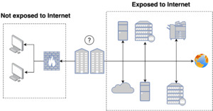
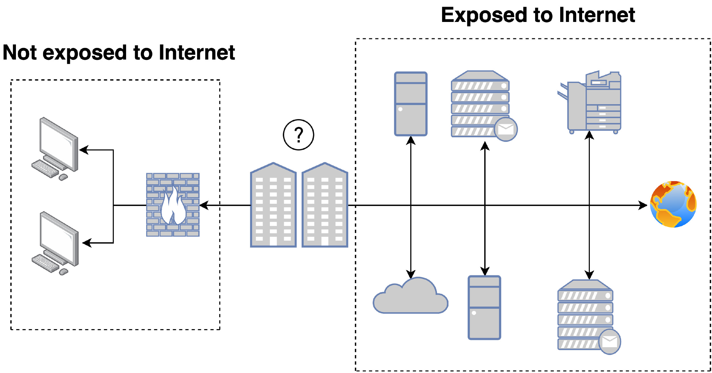
Figure 1 shows the two network segments (Internet-facing and private) for a given organization. We analyze external network posture, which is accessible by anybody with an Internet connection. External network security posture, at a high level, consists of configurations for different protocols, including the port and service behind the protocol, the version of the service, and many other details regarding the state of such external hosts.

Figure 1.Internet-facing and private network segments of an organization

The advantage of our using the external network is that it makes a great deal of information publicly available and does not require information from inside the organization. Hence, it makes it relatively informative and easy to acquire at scale.

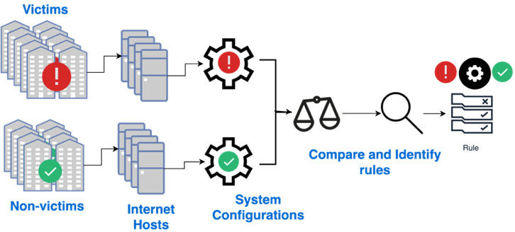
We investigate the extent to which system configuration data can be used to predict the likelihood of a security incident by carefully collecting a group of victim organizations (each of which has reported a security incident) and nonvictim organizations (none of which has reported a security incident) and comparing their external system configuration data (Figure 2).

Figure 2.Contemporary approach in problem domain: collect victim and nonvictim organizations, attribute their assets, and compare rules that discern victim configurations

We hypothesize that the configurations relate, in varying degrees, to the occurrences of hacking or malware incidents. This relationship exists either directly—through evidence that attackers exploited a vulnerability appearing in the external system configuration data—or indirectly—through lack of adequate internal policy and implementation of controls to protect the organization’s assets. The assumption that company culture is correlated with the external system configuration is consistent with previous works. Zhang et al. (2014) and Y. Liu, Sarabi, et al. (2015) have shown that misconfigurations can lead to malicious attacks and can be used to predict security incidents with high positive predictive value. We extend their research using heterogeneous data, holistic methods of host representation, and novel machine learning algorithms. In addition to this, the loose coupling of public data and technique affords readers the ability to apply the methods we describe to other similar data sets. The intuitive statistical concepts and analytical methods our approach uses can easily be used for other cyber risk analyses.

1.2. Cybersecurity primer

This section consists of a brief primer for the more complex ideas presented throughout the rest of the paper.

A computer network is a collection of computers that are connected and share information. A service is an application running a protocol on a computer port, where a protocol is a set of procedures that govern communication in a network and a port is a number between 0 and 65535 that uniquely identifies the service. For example, A file transfer protocol (FTP) service is handled on TCP port 21, and its data transfer can use TCP port 20 as well as dynamic ports depending on the specific configuration.

An organization’s domain is a label that identifies a group of computers (both internal and external) belonging to the organization, e.g., drexel.edu. A subdomain is a label that describes a smaller group of computers belonging to a domain or another subdomain, e.g., www.drexel.edu. The Domain Name System (DNS) converts the domain and subdomain names to corresponding Internet Protocol (IP) addresses and vice versa. A digital asset, in this context, could be an IP address, a domain name, a subdomain name, or the host (computer) behind the IP address that belongs to a particular organization. On-premises assets refer to workstations and servers that an organization maintains itself, while cloud-hosted assets are assets managed by a cloud provider (e.g., GoDaddy, Amazon). The organization size is the number of Internet-facing or publicly exposed hosts for an organization.

Footprinting (e.g., subdomain enumeration) and Internet scanning are reconnaissance processes used to identify hosts, and their network services, that belong to an organization. Services running a misconfigured or vulnerable application on the public Internet provide a typical avenue for a threat actor (e.g., malware) to infiltrate a company’s network, which often leads to a security incident.

A security incident is an act of violating an explicit or implied security policy. Essentially, it is an event that indicates an organization’s information technology (IT) system may have been compromised. A data breach is a security incident in which sensitive, protected, or confidential data are copied, transmitted, viewed, stolen, or used by unauthorized individuals. A victim organization is an organization that has reported a security incident (or data breach). On the other hand, a nonvictim organization is an organization that has not published a security incident. A cohort, within this context, is a collection of victim and nonvictim organizations.

With the analysis in this paper we hope to (1) introduce a novel technique of classifying victim and nonvictim organizations (Section 4.1), (2) identify the criterion that best discriminates between those two classes (Section 4.3), and (3) gauge and compare the performance of the model (Sections 4.2, 4.3, and 5.2). For a longer, more detailed list of cybersecurity terms, please refer to the glossary at the end of the paper.

1.3. Related studies

Durumeric, Wustrow, and Halderman (2013) introduced a tool called ZMap that can be used to scan the public IPv4 (Internet Protocol version 4) space (about 4.2 billion IP addresses) in under an hour. Censys (Durumeric et al. 2015) is a search engine and data processing facility built on top of ZMap that collects structured Internet data every 24 hours. We leveraged Censys (2019) in our analysis to obtain accurate and timely data about the configurations of organizations.

Zhang et al. (2014) and Y. Liu, Sarabi, et al. (2015) conducted separate but related studies with a very similar motivation to our work. Zhang et al. (2014) analyzed the extent to which network mismanagement relates to maliciousness. They show a statistically significant positive correlation (0.64) between mismanagement and maliciousness. They also show that an inferred causal relationship exists between mismanaged networks and labeled malicious systems. Y. Liu, Sarabi, et al. (2015) aimed to proactively predict security incidents—e.g., of the sort that Verizon reports in its annual Data Breach Investigations Reports—using externally observable properties of an organization’s network. Their feature space consists of a diverse set of 258 externally measurable features of a network’s security posture. Among those features are one organization size feature, five misconfiguration features, 180 raw time series maliciousness features, and 72 analyzed time series maliciousness features. These are measurements of malicious activities seen to originate from the network. Their results outperform results to date with a 90 percent true positive rate, 90 percent accuracy, and a 10 percent false positive rate.

Our work is different from the aforementioned analyses in the following ways. First, we use a feature extraction engine that provides more than 1,386 features across 26 protocols, providing a richer feature space. Second, whereas Liu et al. utilized reputation blacklists in their analysis, we do not because it introduces a dependency for external security researchers to report malicious IP addresses. Moreover, such lists would need to be updated frequently to maintain accuracy. Lastly, in Liu et al.'s asset attribution step, they map an organization reported in an incident to a set of IP addresses through a sample IP address of the organization involved in the incident. However, that approach is prone to the introduction of attribution errors due to the large number of IPs controlled by public cloud providers. In our analysis, we attempt to improve upon that method by including contemporary reconnaissance tactics (McClure, Scambray, and Kurtz 2001; Roy et al. 2017; Hassan and Hijazi 2018), in combination with manually verified American Registry for Internet Numbers (ARIN) lookups of digital assets. This modification allows us to locate IP address blocks under multiple owner IDs, and effectively map them to the same organization, much like a contemporary attacker would.

In addition to the aforementioned works, some other malicious activity prediction studies are as follows:

• Sarabi et al. (2015) examined the extent to which an organization’s business details can help forecast its risk of experiencing different types of data incidents. They show that it is difficult to assert, with certainty, the types of incidents a particular organization is likely to face.

• Y. Liu, Zhang, et al. (2015) applied a support vector machine to a set of reputation blacklists to generate predictions for future security incidents that may happen to a network.

• Soska and Christin (2014) apply machine learning to predict whether a website may turn malicious and show that their method can achieve a 67 percent true positive rate and a 17 percent false positive rate.

1.4. Problem definition and scope

As mentioned earlier, our goal is to propose a system of security posture–based forecasting by profiling network configurations that are associated with victim organizations. To that end, we employ a numeric interpretation of the configurations for such systems. We then set up a machine learning problem using the configurations as features and the report label as the target. These raw feature vectors compile down to the organizations’ risk vectors. The risk vectors then predict whether an organization will experience a security incident.

Our scope does not include performing any of the following (similar to previous works, such as Sarabi [2018] and Y. Liu, Zhang, et al. [2015b]):

Intrusion point detection. In this work, we do not aim to identify vulnerabilities in Internet hosts, nor do we attempt to uncover possible attack vectors used by malicious agents. Despite that fact, our results and previous works (Sarabi 2018; Y. Liu, Zhang, et al. 2015) reveal that inadequately managed systems have noticeably high degrees of correlation with organizations that report security incidents.

Collection of measurements. This work brings together analyses from numerous data sources, but other than digital footprinting, it does not conduct novel measurements—that is, we do not scan the organizations’ network ourselves.

Use of internal data. We do not analyze cyber insurance applications, internal application logs, or any other information that is not available to an external attacker. Instead, our analysis focuses on outside-in data, i.e., the external network configurations of an organization.

1.5. Contributions

Current work, both in academia (Aditya, Grzonkowski, and Le-Khac 2018; Y. Liu, Zhang, et al. 2015; Zhang et al. 2014) and in the industry (FICO; BitSight [https://www.bitsight.com/]; Security Scorecard [https://securityscorecard.com/]) makes use of a similar pipeline for collecting information about organizations, forming the risk vectors, and analyzing the most effective discrimination rules (Sun et al. 2019). In that pipeline (Figure 2), a set of victim and nonvictim organizations is first identified. That step is followed by attributing their digital assets and configurations on those assets. The configurations are then compared to identify the rules that provide the best discrimination. Using Figure 2 as a starting point, we contribute to the general pipeline in the following ways (Figure 3).

• Heterogeneous nonvictim collection. To provide an accurate analysis of victim organizations, we compare victims against a set of nonvictim organizations. To avoid selection bias, we collect nonvictim organizations using three different methods (described later).

• Improved asset attribution. Footprinting is the process of identifying the assets of an organization. Since there is no single “ground-truth” data source of external asset ownership and digital asset usage on the public Internet, we use contemporary reconnaissance tools to attribute digital assets, in much the same way an attacker would.

• More holistic host representation. Recent studies (Y. Liu, Zhang, et al. 2015; Zhang et al. 2014) rely on a feature space of some 260 or fewer features. Our feature space spans 1,386 features, representing more detailed configuration data from the hosts. This expanded feature space affords us the ability to conduct our analysis at a higher resolution than previously possible.

• State-of-the-art machine learning for outlier detection. Our work applies an isolation forest (an outlier detection algorithm) to the problem domain to identify system configurations of interest. Such an outlier detection algorithm allows us to effectively reduce the data space to a set of hosts that is about 12 percent of the original size while achieving an incident prediction accuracy of 0.73 ± 0.06, an F1-score of 0.73 ± 0.06, and a false positive rate of 0.25 ± 0.10.

Figure 3.Novel contributions to the contemporary approach

1.6. Outline

The rest of this paper is structured as follows. In Section 2, we discuss the cyber risk and insurance dimensions of the work. Section 3 describes the data pipeline (gathering the network information from Censys and extracting the features from the hosts). In Section 4, we analyze the data by setting up the classification problem, selecting the system configurations of interest, and generating the feature importance charts. Finally, Section 5 concludes the analysis and lists some avenues for future work.

2. CYBER RISK

2.1. Definition

Our goal is to provide a method of determining the probability of a cyber incident with the highest possible confidence. Cyber risk, within the realm of cyber insurance, is often presented in terms of the likelihood that a given organization will experience a cybersecurity loss event multiplied by the magnitude of that cyber loss event, that is,

$$R = P*M,$$

where $R$ is the cyber risk, $P$ is the probability of a cyber event, and $M$ is the magnitude of the loss. For this discussion, however, we exclusively consider the likelihood of the cyber loss event ($P$) portion of cyber risk. Although the different types of cyber loss events number in the dozens, we focus on cyber losses stemming from remote attacks against Internet-connected computer systems or networks. We also define a cyber risk vector as a numerical representation of this cyber risk. Hence, the (cyber) risk vector is built from data about organizations’ external system configurations.

2.2. Cyber insurance

Cyber insurance underwriters frequently use industry class (finance, retail, healthcare, education) in addition to gross revenue and the number of data records held to evaluate cyber risk. Underwriting evaluations also rely on the use of data from insurance applications that prospective customers fill out. Today, automated cyber risk analyses using external system configuration data are available from several companies, including FICO Enterprise Security Suite, BitSight, SecurityScorecard, and UpGuard.

FICO’s Cyber Risk Score (https://cyberguide.advisenltd.com/fico/) relies on a diverse set of Internet-scale security signals to determine an organization’s risk profile. This information is then used to train a machine learning model that produces a risk score that forecasts the likelihood of a future breach event. SecurityScorecard analyzes the cyber risk of an organization using outside-in data. The platform gathers security data and grades organizations from A to F across 10 security categories (web application security, network security, endpoint security, DNS health, patching cadence, hacker chatter, IP reputation, leaked credentials, social engineering, and cubit score). Their goal is to discover organizations’ external security posture from the perspective of a hacker, business partner, or customer. BitSight uses externally observable data on compromised systems, security diligence, user behavior, and public disclosures to compute an organization’s security rating. BitSight’s security ratings consist of event data and diligence data. Whereas event data comprise evidence of botnet infections, spam messages, malware servers, unsolicited communication, and other indicators of compromise, diligence data include information about security diligence, such as SSL (Secure Sockets Layer), SPF (Sender Policy Framework), and DKIM (DomainKeys Identified Mail) configurations. Finally, UpGuard uses most of the aforementioned data types but also monitors so-called hacker chatter (e.g., social networks).

2.3. Challenge of asset attribution

One issue that academia and the industry still face is how to effectively attribute digital assets (Y. Liu, Zhang, et al. 2015; Zhang et al. 2014). Most industry professionals attempt to solve that by manual confirmation of an organization’s Internet-visible network assets. There is no apparent automated method to gather an organization’s digital resources, however. We use contemporary reconnaissance tactics to address the issue (see McClure, Scambray, and Kurtz 2001; Roy et al. 2017; Hassan and Hijazi 2018).

3. DATA

3.1. Data collection

We used a set of data sources, discussed in this section, to aid in identifying organizations of interest, attributing hosts to them, and collecting the attributed hosts. We selected the sources based on integration capability. Figure 4 shows the data collection pipeline.

Figure 4.Pipeline collects victim and nonvictim data to map, manage, and extract features from their assets

The pipeline is broken down into four steps: cohort selection, host attribution, host collection, and feature engineering.

Step 1. Cohort selection. The time range we employ in this analysis is January 1, 2017–January 1, 2019. An organization is classified as a victim or nonvictim within this time window (incident report window). The cohort set consists of one victim and three nonvictim subsets.

Figure 5.Victim organization collection pipeline

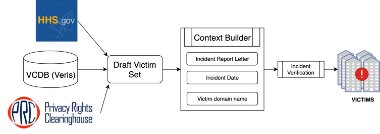
Victim organization collection. The victim organizations are located through security incident data sources. Security incident data sources contain ground-truth security incident information, including the organization that reported the security incident, the report date, and many more fields that add context to the incident. Among the many sources that provide such information, we selected three based on update frequency, data format, ease of access, and overall integration capability: Privacy Rights Clearinghouse, VERIS Community Database, and the U.S. Department of Health and Human Services. The use of three different security incident data sources reduces the bias toward any particular reporting agency, similar to Liu et al. (2015). From 263 incidents (176 Privacy Rights Clearinghouse incidents, 84 VERIS incidents, and three Health and Human Services incidents) that match our selection criteria, we randomly sampled 200 for this study.

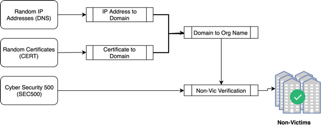
Nonvictim organization collection. As this work analyzes the common traits among Internet-facing systems of victim organizations and compares those traits with those of nonvictim organizations, we must generate a sublist composed of nonvictims. Nonvictim organizations are collected through three different methods, shown in Figure 6. Those methods entail sampling from three sources: Cybersecurity Ventures’ Security 500 (SEC500); digital certificates (CERTs); and domains from reverse IP address resolutions (DNS).

Figure 6.Nonvictim organization collection pipeline

Cybersecurity Ventures (https://cybersecurityventures.com/), a cyber economy researcher and publisher, annually selects the top (“most innovative”) 500 organizations in the field of cybersecurity. A sample of the domain names present in that list is used as a subset of nonvictim organizations.

The second method of identifying nonvictim organizations is to sample subjects from digital certificates. A uniformly sampled batch of 15,000 IP addresses is collected from a Censys table containing 160 million IP addresses. From this batch, the digital certificates are used to locate the subject fields, which are then associated with a domain name.

For the third method, the batch is again utilized to sample a host and a reverse lookup of the IP address randomly. This method would immediately return a domain name on the public IPv4 space.

We selected 200 nonvictim organizations using each of the three methods above, ensuring that none of them appears in any of the victim data sources. At this point, we have collected a cohort of 800 organizations (785 unique), where each organization contains a name, a victim/nonvictim label, one sample domain, and a lookup date.

Step 2. Host attribution (footprinting). Footprinting, or host (asset) attribution, is the process of finding digital assets (IPv4 addresses and domain names) associated with a particular organization. A custom component was built that collected, curated, and stored the digital assets for the cohort. The tools used to accomplish this are the same as those used by penetration testers, ethical hackers, and malicious actors for reconnaissance (Pentester Land 2018; Hudak 2017). Next, we associate a set of subdomains to each domain name in a process called subdomain enumeration: for example, if the domain is ibm.com, some possible subdomains include research.ibm.com and dev.ibm.com. The IP address resolution process resulted in 2.3 million total subdomains. Of those, 400,000 are nonresolvable. Hence, we have 1.9 million IPv4 addresses that are attributed to the cohort.

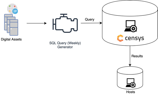
Step 3. Host collection. The host collection component constructs queries from the digital assets (domain and IP addresses) for each organization, which are then used to collect data about the associated hosts from Censys. Figure 7 shows the host collection process. The analysis collected 714,244 hosts across all the organizations in the cohort.

Figure 7.Host collection stage using Censys (Durumeric et al. 2015)

Step 4. Feature engineering. Once the hosts have been collected from Censys, a feature engineering component converts them into feature vectors. For our study, a feature is defined as a mathematically analyzable property of an observation. Each feature vector should ideally be a numerical representation of the Internet-facing system configurations present on each host. The process is shown in Figure 8. The feature extraction component uses the 9,899 fields available in Censys to extract 1,386 features. The engine handles the following feature types:

• Numeric fields: These are direct transfers of numeric fields from the Censys data model, e.g., the validity length in seconds for an HTTPS (HyperText Transfer Protocol Secure) certificate.

• Boolean fields: These are converted to {0, 1} for a mathematical representation, e.g., RUNNING P22 SSH would equal 1 if true or 0 if false.

• Enumerated fields: These are one-hot encoded for the possible values for that field, e.g., TLS CERT VERSION could be 1.0, 1.1, and 1.2. These are converted to three Boolean features: TLS VERSION 1.0, TLS VERSION 1.1, and TLS VERSION 1.2, which have values {0, 1}.

• Text fields: For these fields, we looked up the top 10 to 20 values through the Censys report tool and treated them as enumerated fields.

Figure 8.Feature engineering stage to extract features from 26 protocols

In addition to the features from the 26 protocols, we included the following features:

• ORG_SIZE: number of hosts an organization owns.

• NUM_PORTS: number of ports that are running a service on a host.

• METADATA_DESCRIPTION: synonym for the operating system.

• COMPANY_NAME_IN_ASN: the feature that allows us to differentiate the host as on-premises or in the cloud.

• AUTONOMOUS_SYSTEM: if the host is in the cloud, checks for more common cloud providers, such as AWS, Google, GoDaddy.

At this stage, we have collected 714,244 hosts across the 785 organizations. We have represented each host as a feature vector of length 1,386.

4. PROBLEM MODELING

Once we have selected the cohort and attributed the Internet-facing assets to their respective organizations, we apply numerous statistical tools, models, and algorithms in order to categorize/label the data. We then analyze the performance of the models and the rules that are most effective in discriminating between the two types of organizations (and their host machines) and thus most useful for quantifying the probability of a cybersecurity incident.

4.1. Experimental setup

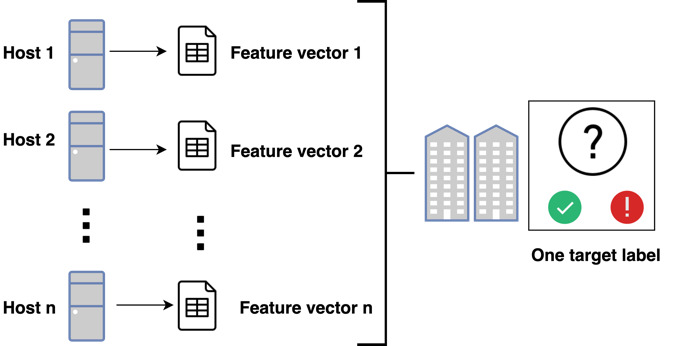
We now set up the experiment as a machine learning problem. The target label is whether an organization has or has not reported a security incident (a victim organization or a nonvictim organization). The features are the individual host configurations in an organization’s network. The first obstacle we seek to overcome at this phase stems from the fact that the labels victim organization and nonvictim organization are at the organization level, but the features we are analyzing are at the system level (see Figure 9). In short, we face the challenge of mapping the features to the label when the features and labels are at different resolutions, namely, the host and the organization, respectively. Averaging all the features across an organization’s hosts would not work because any distinctive feature associated with a host will be lost in a large enough organization, which is the case for numerous organizations in our cohort.

Figure 9.Challenge with the experimental setup: Features and target label at different levels

Moreover, the features we are most interested in are misconfigurations, which are common in the minority in a network. Another approach would be to assign the label to each of an organization’s hosts. However, that again would prove suboptimal for two reasons. First, it would erase the idiosyncrasies by overloading the model with numerous hosts with configurations that are not immediately relevant to the task of assessing organizational risk. Second, if an organization is large enough, looking at all of the hosts would be time-consuming, impractical, and expensive.

4.2. Outlier detection and isolation forest

We use unsupervised anomaly detection to mitigate the issues mentioned in Subsection 4.1. Outliers are observations that occur rarely in a data sample, and hence, they are statistically different from most other observations. Outlier detection (unsupervised anomaly detection) is a method of identifying observations that are outliers. Using that approach, we can identify hosts that are a representative sample of machines in a network (inliers) and hosts that are different (outliers) from most of the organization’s hosts. Two conventional outlier detection approaches are employed. First, univariate outlier detection is used to locate the extreme value for one feature (variable), e.g., the box plot rule. Second, multivariate outlier detection is used to locate the extreme value across multiple features (using, e.g., Mahalanobis distance, one-class support vector machine, elliptic envelope, or local outlier factor).

Most existing model-based approaches to outlier detection construct a profile of regular instances (F. T. Liu, Ting, and Zhou 2008) and identify instances that do not conform to the typical profile. An isolation forest is an ensemble decision tree algorithm that identifies anomalies instead of profiling normal points explicitly. The algorithm works as follows. First, for every base estimator (decision tree), a sample of 256 data points is selected from the data set. Second, a random sample set of features with a size equal to the square root of the feature space (generally, both anomalies and outliers can be explained by a few features) is selected. Third, a random feature from that set is selected. Fourth, a random value between the minimum and maximum is selected for that feature. Fifth, the data are split on that value for that feature. Finally, the preceding steps are repeated until the sample data points are fully separated. After these steps, each data point will have a set of associated depths (wherein the decision tree, this data point is separated from the others). The intuition is that anomalies/outliers will produce noticeably shorter paths on random partitions of the feature space, as shown in Figures 10 and 11.

Figure 10.Isolation forest (F. T. Liu, Ting, and Zhou 2008): Isolating x_i (left) and x_o (right)

Figure 11.Isolation forest (F. T. Liu, Ting, and Zhou 2008): Average depths converge

Because outliers will be isolated more easily on random partitions of the feature space, the expectation (mean) for this depth will be smaller for outliers than for other observations. The scoring function used in the isolation forest algorithm is

$$s(x,\ n) = 2^{- E\lbrack h(x)\rbrack/c(n)},$$

where $s(x,\ n)$ is the outlier score for a data point $x$ in the sample data of size $n$; $E\lbrack \ \rbrack$ is the expectation (mean) of a random value across all trees; $h(x)$ is the depth of data point $x$; and $c(n)$ is the average path length of unsuccessful search in a binary search tree (i.e., the average height of the base trees). The data point $x$ may be classified based on the value of $E\lbrack h(x)\rbrack$. First, if $E\lbrack h(x)\rbrack = n-1$, then $s(x,n)$ is near 0, i.e., the data point is always hard to isolate, and hence is an inlier. Second, if $E\lbrack h(x)\rbrack = 0$ then $s(x,n)$ is near 1, i.e., the data point is always easy to isolate, and hence is an outlier. Third, if $E\lbrack h(x)\rbrack = c(n)$, then $s(x,n)$ is near 0.5, i.e., the data point is ambiguous. This value is the decision threshold.

The isolation forest algorithm was selected for two reasons. First, it does not need to learn the underlying distribution (i.e., it is not a generative model), and second, it does not require any parameters other than the data and number of decision trees, which reduces developer’s bias.

An isolation forest model with 200 base estimators is learned with the host feature vectors and used to identify outliers and inliers for each organization. We identified 45,329 outliers and 45,225 inliers from the 714,244 total host count. These liers are about 6 percent outliers and 6 percent inliers, which reduced our data space to about 12 percent of the original size.

Outlier versus inlier analysis. Having identified sample liers, we next seek to assess whether the criteria that make a host an outlier transcend organizational boundaries. That is, if a host is an outlier in a particular organization, will it tend to be an outlier in another organization? To perform that analysis, we select a set of 20 sample outliers and 20 sample inliers for each organization from the cohort as our data set, resulting in 7,208 inliers and 7,312 outliers. This method is set up as a binary classification problem where the class label is 1 for outliers and 0 for inliers. An optimal maximum tree depth of 15 is tuned on a sample of 200 randomly selected organizations (20 inliers and 20 outliers from each organization). With this parameter, we use all 785 organizations to generate the receiver operating characteristic (ROC) curve for the true positive rate and false positive rate values (Figure 12).

Figure 12.Outlier versus inlier classification ROC curve

During the analysis, we saw that the performance for discerning outliers from inliers depends on organization size (i.e., number of hosts in an organization). Hence, the analysis is repeated for organizations grouped by size.

Figure 13 shows the ROC curves for different-sized organizations. We calculate the optimal threshold using Youden’s J statistic. Using the optimal threshold (labeled as the Mean Op. Pt. in the ROC graphs), we can gauge the model’s performance. Table 1 shows the performance metrics (F1-score, accuracy, false positive rate, number of important features, and support for outliers and inliers) for the analysis. The host attribution step during data collection is susceptible to historical noise due to the reassignment of IP addresses to new assets and organizations. To counter this, the above analysis is repeated for only the hosts attributed using the organization domain names (found in the subject portion of the hosts’ digital certificates). Attribution through domain name is more historically reliable, but it is less likely to capture hosts that do not have a certificate (attackers will more likely leverage because of less visibility) (McClure, Scambray, and Kurtz 2001; Roy et al. 2017; Hassan and Hijazi 2018). Table 2 shows the performance of the model using the optimal discrimination threshold.

Figure 13.Outlier versus inlier classification for different-sized organizations

From the curves in Figure 13, we see the following. First, outliers are more easily identified in larger organizations versus smaller ones. As the organization size increases, the area under the ROC increases, and the number of essential features required to predict the target label decreases (Figure 13, Table 1, and Table 2). Second, if one does not know the organization size, then for a given set of hosts, the model can use 41 features to assign an outlier label with 0.84 ± 0.01 accuracy and a 0.18 ± 0.04 false positive rate. These statements are consistent for the hosts that are attributed through only certificates as well.

Victim versus nonvictim host analysis. We assign the organization label to these representative lier samples (inliers and outliers). This method enables us to set up three separate classification scenarios: one victim cohort subset against three nonvictim cohort subsets, as a result of the three different nonvictim organizations. The method is repeated for the two types of liers (outliers and inliers) separately, as shown in Figure 14.

Figure 14.Host classification using outlier and inlier hosts

Hence, we have trained six models, two liers (outlier and inlier) for three different nonvictim selection scenarios. The inlier models compare the most typical system configurations of the victim against the nonvictim organizations while the outlier models compare the most atypical. This separation ensures that the organizations’ idiosyncratic configurations are captured more effectively. To economize, we select a maximum of 350 samples per lier per organization for the analysis. These models are used to generate the ROC curves shown in Figure 15. The performance of the model at the optimal discrimination threshold is tabulated in Tables 3 and 4 for the two lier classification problems.

Figure 15.Randomly sampled nonvictim versus victim host classification using all attributions: (a) DNS inliers; (b) DNS outliers; (c) CERT inliers; (d) CERT outliers; (e) SEC500 inliers; (f) SEC500 outliers

Looking at the curves in Figure 15, we can see that both lier analyses for the DNS and CERT cohort subsets perform well (discernable against VICTIM subset). However, the SEC500 models do not perform as well. This performance is due to the organization size (i.e., the large sizes of the nonvictim organizations) being an important feature for the former two cohorts.

Victim versus nonvictim organization analysis. Once the inlier and outlier hosts are attributed to the victim and nonvictim organizations, the next challenge is to condense the hosts’ probability scores into an organizational risk profile. The intuition behind such a profile is that it should be a “summary” of the sample liers’ probability scores. We approximate the risk profile as the summary statistics for the distribution of scores across the lier machines. The four summary statistics are (1) the five quartiles: [0, 25, 50, 75, 100]; (2) the score average; (3) the score variance; and (4) the number of scores. Those result in 16 summary statistics (eight per outlier and inlier) for each organization that we can now use to train a risk model. The summary of the training probabilities is used for training risk profiles, and the same is applied for the testing probabilities, as shown in Figure 16. These are used to train a random forest risk profile model that predicts the likelihood of experiencing a reportable security incident based on the lier samples. Figure 17 shows the ROC curves for the models run against each cohort subset. Table 5 shows the performance of this model at the optimal discrimination threshold.

Figure 16.Organization classification using the probability distributions from outlier and inlier classifications

Figure 17.Victim versus nonvictim organization classification using all attributions: (a) DNS, (b) CERT, (c) SEC500

Through the individual lier classification (Subsection 4.2), it is not apparent which type of lier is better for security incident prediction. In other words, separately analyzing the sample inliers or sample outliers will not lead to the most optimal classification performance. However, when combined to predict the label for an organization, the model performs better.

We can see that summarizing the scores for individual liers into a risk vector shows an average classification performance of 0.73 ± 0.06 accuracy, a 0.73 ± 0.06 F1-score, and a 0.25 ± 0.10 false positive rate (Figure 17 and Table 5). This outcome is consistent with results for the certificate-attributed hosts as well.

4.3. Analysis of results

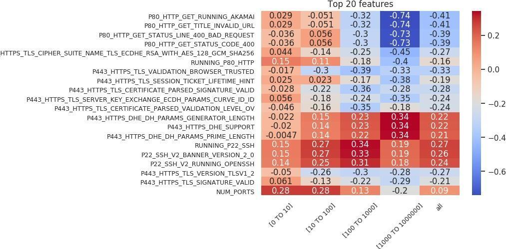
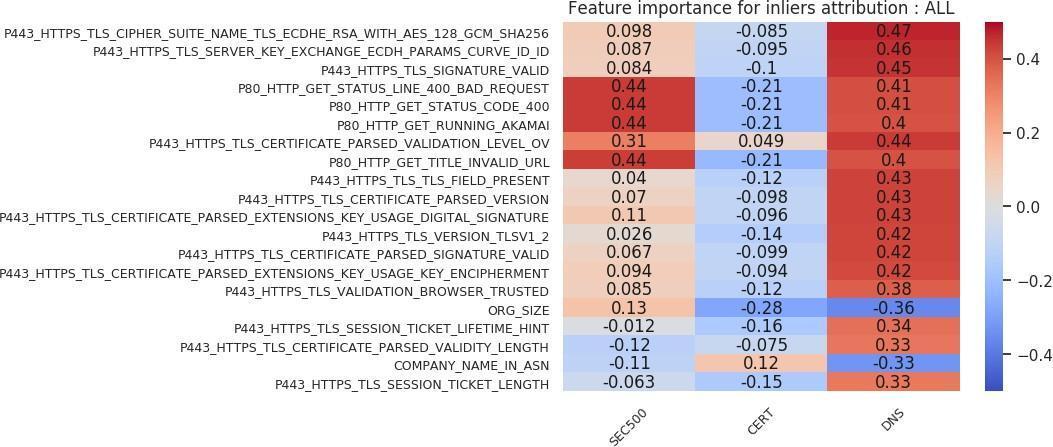
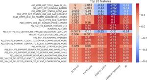
Sarabi and Liu (2018) wrote that “in the context of security, simply building black-box models is not sufficient, as one cannot readily infer why a model is making a certain prediction.” To fully answer the question of what makes an outlier in our feature space, we need to identify the rules that are important in the classification. We take the features that are important in the random forest model and combine them with the Spearman correlation between the feature and the target label to identify these rules. This collection is then sorted based on correlation, and the top 20 are presented as a feature importance chart. The feature importance charts for the outlier versus inlier classification are shown in Figures 18 and 19. On the x-axis of each chart, we can see the organization size associated with the model, while the y-axis represents the features. Each entry shows how correlated that important feature was with the target outlier label.

Figure 18.Outlier versus inlier classification feature importance chart using all attributions

Figure 19.Outlier versus inlier classification feature importance chart using only certificate attributions

Numerous theories can be applied to explain the charts in Figures 18 and 19. For the sake of brevity, we will analyze only a small subset of the features. The following are positively correlated with the outlier label: first, running an SSH (Secure Shell) server (most of the top 20 features are taken up by the SSH protocol); second, an HTTPS web server configured with “P443 HTTPS DHE” (Diffie–Hellman) features; and third, a web server on port 80 that returns a “200” (OK).

The following are negatively correlated with the outlier label: first, an HTTPS service with a valid, browser-trusted certificate; second, an HTTPS web server that is not configured with Diffie–Hellman features; and third, using an “Akamai Global Host” web server on port 80 that returns a “400” bad request.

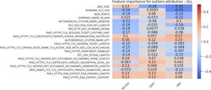
We can extend the same feature importance chart analysis to victim versus nonvictim host analysis. Figures 20, 21, 22, and 23 show those charts. We deduce the following from the inlier charts (Figures 20 and 21). First, larger organization sizes, again depending on the cohort, are positively correlated with the victim label. Second, in the feature importance chart using all attribution techniques (Figure 20), we see that compared to the VICTIM cohort, the DNS cohort has far fewer HTTPS certificates. That result is a direct example of how selecting a nonvictim cohort can be a difficult task, and of how selecting a representative cohort is very subjective. In this case, the inlier model has identified the criterion to be that victim organizations’ profiles contain more certificates than those of nonvictim organizations. That result, depending on what the analyst wants the model to learn, may or may not be an issue. Third, using an “Akamai Global Host” web server with a “400” response is positively correlated with the victim label in the SEC500 and DNS subsets, but negatively correlated (or indifferent) with the CERT subset. Fourth, an HTTPS certificate that has organization-level validation (“VALIDATION LEVEL OV”) is positively correlated with the victim label in all subsets. Fifth, running an HTTPS certificate issued by Comodo or GeoTrust is slightly positively correlated with the victim label. Sixth, the length of validity for the HTTPS certificate is negatively correlated with the victim label. This result means a longer validity length is associated with nonvictim organizations.

Figure 20.Victim versus nonvictim inlier host classification using all attributions

Figure 21.Victim versus nonvictim inlier host classification using only certificate attributions

Figure 22.Victim versus nonvictim outlier host classification using all attributions

Figure 23.Victim versus nonvictim outlier host classification using only certificate attributions

Again, many theories can be developed based on outliers in Figures 22 and 23. The following are a select sample. First, larger organization sizes are negatively correlated with the victim label for the CERT and DNS cohorts. However, they are positively correlated with the victim label in the SEC500 analysis. That result means that victim organizations tend to be smaller in size than randomly sampled organizations from the Internet. Second, running an SSH server is negatively correlated with the victim label in the SEC500 and DNS cohort subsets, and indifferent in the CERT subset. Third, running an HTTPS server that has “P443 HTTPS RSA EXPORT SUPPORT” (the FREAK vulnerability, which allows an attacker to force export-grade encryption [Censys, n.d.]) enabled is slightly positively correlated with the victim label. Fourth, running an HTTPS certificate with Diffie–Hellman or Key Encipherment is slightly positively correlated with the victim label.

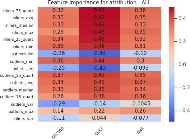
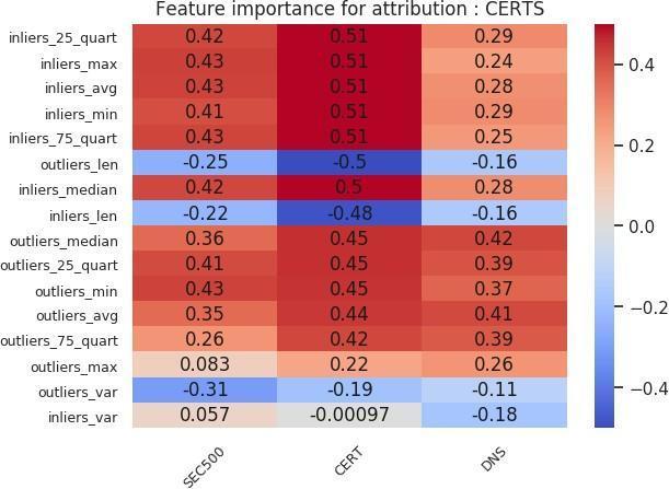
Figures 24 and 25 show the feature importance charts for the organization-level analysis. We can draw several conclusions. First, the inlier statistics are strongly positively correlated with the victim label in the CERT subset. However, in the other subsets, the correlation is equally distributed among the liers. Moreover, in the DNS subset, for the certificate-only attribution, outlier statistics are positively correlated with the target label. Second, having more outliers is negatively correlated across all cohort subsets. That does not extend to inliers since the number of inliers was chosen to match the number of outliers. Third, high variance in the probability scores of the outliers is negatively correlated with the victim label.

Figure 24.Victim versus nonvictim organization classification using all attributions

Figure 25.Victim versus nonvictim organization classification using only certificate attributions

4.4. Discussion

The analysis of the results (feature importance charts) exemplifies the fact that we do not conduct vulnerability analysis but rather profile network postures, since the features attributed to the victim organizations’ systems were predominantly benign configurations. We can see that the SSH protocol is positively correlated with the outlier label but negatively correlated with the victim label. This correlation is consistent with the understanding that the protocol is rare but also secure. However, a misconfigured HTTPS server (Diffie–Hellman [Adrian et al. 2015] and FREAK [Censys, n.d.]) is positively correlated with both the outlier label and the victim label. We found that a known vulnerability (FREAK) is slightly positively correlated with the victim label in almost all cohort subsets. Such a correlation indicates that victim organizations have undermanaged networks, as previous studies have found (Zhang et al. 2014; Y. Liu, Sarabi, et al. 2015). Moreover, the indication we find is in line with previous work that found untrusted HTTPS to be the most crucial mismanagement feature (Zhang et al. 2014; Y. Liu, Sarabi, et al. 2015). Finally, the performance we achieved is also consistent with prior studies that have used configuration information (Y. Liu, Sarabi, et al. 2015; Wang et al. 2014).

5. CONCLUSION

5.1. Summary of contributions

Referring back to the novel contributions illustrated in Figure 3, we take away the following. First, the heterogeneous nonvictim collection methods that show us the selected method of nonvictim collection do have an impact on the outcome of the most important rules (highly correlated system configurations) in the classification stage. Second, the state-of-the-art outlier detection techniques show that nonvictim organizations tend to have more outliers and higher variance in those outliers than victim organizations. Third, the novel footprinting techniques reveal that SSH is a secure outlier (this was not visible without this attribution technique seen in the domain name–only analysis). Fourth, the holistic host system representation (a result of the size of the feature space) allows us to generate the feature importance charts with greater detail and dig even deeper into each protocol. In addition to these contributions, this analysis also enables the expansion of effective risk management sectors like cyber insurance, and aids underwriters in better customization of their policies by introducing a novel method by which to approach the Internet security problem.

5.2. Performance comparison

The works of Soska and Christin (2014) and Y. Liu, Zhang, et al. (2015) (Subsection 1.3) are the two most similar in terms of technical approach to our analysis. Table 6 compares our model’s performance with theirs. From Table 6, it is evident that Liu et al.'s model demonstrates higher accuracy with a lower false positive rate than our analysis. We attribute this to the use of maliciousness features identified by third-party sources, as it is much easier to predict the likelihood of a security incident if an organization’s network is known to be malicious. Figure 26 illustrates this. In that figure, the performance of the mismanagement, most similar to our feature space, is worse than that of the other features. We covered the downsides of using reputation blacklists in Subsection 1.3; however, that remains an avenue for future work.

Figure 26.Y. Liu, Zhang, et al. (2015) model performance of separate features

5.3. Future work

The work described in this paper could be extended in several directions. First, although we performed the posture analysis by taking a snapshot of an organization’s network at a given moment, previous works (Y. Liu, Zhang, et al. 2015; Zhang et al. 2014) analyzed a time series of network snapshots. Time series analysis is an excellent direction for future work as it accounts for the dynamic nature of a network configuration over a time period. Second, in our analysis, we represented an organization as a summary statistic vector of the individual host probabilities. That representation was a solution to the resolution issue where the features and target labels were at different levels. However, that approach is suboptimal because of the loss of networks’ inter-host configuration information. An ideal, more holistic approach is left as an avenue for future work. Third, as we mentioned previously, selecting nonvictims is a challenging task. Moreover, now that we have found that the sampling technique affects the rules that discern victim organizations from nonvictim organizations, we need to collect more nonvictims using other techniques for analysis.

Previous papers (Y. Liu, Zhang, et al. 2015; Zhang et al. 2014; Sun et al. 2019) have made the case that the security community should pay attention to network configurations to maintain the health of the public Internet. But coming up with a way to predict security incidents within organizations’ infrastructure on the Internet is a rather complicated endeavor for the many reasons mentioned in this paper. In addition to those challenges, compared with internal network information, external posture data do not reveal much about an organization’s state.

In this paper, we collect external network posture information for a cohort of victim and nonvictim organizations. We investigate the extent to which those publicly available configurations can be used to predict the likelihood of a security incident. Finally, we compare and contrast the performance of the model we built against other contemporary models in the same problem space.

ACKNOWLEDGMENT

The authors gratefully acknowledge support from the Casualty Actuarial Society. The authors would also like to acknowledge the maintainers of the data sources used in this analysis, including (1) Censys for the host-level information and (2) RiskIQ PassiveTotal (https://www.riskiq.com/), BinaryEdge (https://www.binaryedge.io/), SecurityTrails (https://securitytrails.com/), and VirusTotal for subdomain enumeration information.

APPENDIX

Design Decisions

Due to the relative novelty of the problem, there are no contemporary data collection standards. And that is only exaggerated when dealing with a large data set such as the one here. Our design decision process included some assumptions as well as certain challenges. The decisions are categorized based on the challenges that we encountered: cohort selection, host attribution, host collection, feature engineering, and general.

Design Decision 1: Cohort Selection

The design decisions made in the cohort selection stage are as follows:

1. We make the assumption that organizations that have not reported a security incident are exemplary of a “good” security posture. As Y. Liu, Sarabi, et al. (2015) have shown, there are numerous cases where this does not hold. Three cases are likely. First, organizations might have experienced an incident but it went unreported due to intentional or unintentional negligence. An example of that could be a data breach where the data involved are not sufficient (number of records, exposed credit card info, etc.) to report an incident. Second, organizations might have reported an incident close to the report window but not within it. One of the requirements to be considered a victim organization is to have reported an incident in the incident report window. Third, some Cybersecurity 500 organizations had hosts that are honeypots. Honeypots are hosts that are intentionally left vulnerable to lure attackers away from other real hosts. This can lead to incorrect learning as these vulnerable hosts will be associated with the nonvictim subset.

2. This analysis assumes that the three victim data sources are an exhaustive representation of all victims that have reported security incidents. However, the lists are certainly not exhaustive.

3. As mentioned earlier, the selection of organizations with an international presence has certain issues. To mitigate this, we selected only organizations with a major office in the United States, regardless of where most of their business was conducted. We leave dealing with incidents outside of the United States as a direction of future work.

4. During the nonvictim cohort selection, this analysis avoided cloud providers (Amazon Web Services, GoDaddy, etc.) for the reason that the “ownership” for the configurations that appear in Censys would be uncertain. Again, analyzing the risk profiles of different cloud providers is left as a direction for future work.

As the above list shows, it is quite hard to collect sample organizations that have a “good” external network posture. However, there is one source of ground truth, which is that victim organizations have reported an incident. Therefore, a significant amount of scrutiny is necessary to ensure that the victim organizations are exemplary of “bad” network postures.

Design Decision 2: Host Attribution

The design decisions made during the host attribution stage are as follows. First, the domain name attribution step does not account for organizations that have more than one domain. Incorporating more than one domain name per organization is left as a direction for future work. Second, during the subdomain enumeration step, no guaranteed check is done to see if the subdomains found are updated/registered before or after the lookup date. Given the scope of the time frame and resources, we did not conduct a historical attribution of the IP addresses. A direction for future work would be to use Rapid7 Open Data (https://opendata.rapid7.com/) to check for historical data points. Third, during the subdomain resolution step, the list of resolvers used as a parameter for massdns had some malicious servers. These are name servers that are intentionally returning incorrect IPv4 addresses for the supplied subdomains. To mitigate this issue, we collected 10 reliable name server lists and ran each subdomain against five randomly selected groups. If four or more of the five groups return the same IP address for a subdomain, we take that value; otherwise we drop that subdomain—similar to a majority vote problem. Even though this back-of-the-envelope calculation yielded good results, this is left as a direction for future work.

Ideally, this footprinting technique should efficiently convert an organization name into a domain, or set of domains, that has a high level of confidence of correctly attributing all the public digital resources. However, even with the methods described here, there is still a possibility of false attributions and an even greater likelihood of missed detection when it comes to accurately identifying organization assets. This is because locating all the assets for an organization is a difficult endeavor as there is no ground truth to compare to.

Design Decision 3: Host Collection

Design decisions made in the host collection stage are as follows:

1. We make the assumption that the hosts that have been attributed to the organizations exist in Censys. However, that might not be the case as the company might have blacklisted Censys’s probes.

2. There is a cost associated with running a query against BigQuery’s API. Due to the fiscal constraints, running daily queries was not a feasible option. To make the step more affordable, we did an aggregated weekly lookup instead of daily lookups. The assumption here is that weekly lookups are close enough to daily looks not to skew the results; however, there are no scientific tests to ensure that this is the case.

Design Decision 4: Feature Engineering

During the feature engineering stage, we made the following design decisions:

1. There lies a subtle issue in our feature engineering technique. The lack of features that describe certain protocols as deeply as others leaves a certain imbalance in the way in which protocols dominate the feature space. Building a balanced scheme to extract reliable features from outside-in network posture data is left as a direction for future work.

2. This analysis focused on host-based features. However, inter-host-based (organization-level) features, such as the ratio of hosts that are on the cloud, could prove useful and are a good direction for future work.

Design Decision 5: General

Here are two general design decisions that are not mentioned above:

1. A huge challenge, also mentioned in Liu et al.'s (2015) work, is the challenge of acquiring high-quality incident data. This results in a feature space we cannot more deeply analyze with confidence. First mentioned in Liu et al. (2015), this would not be an issue if a more systematic incident reporting model were in place.

2. Given the resource constraints, we had neither the time nor the resources to do a full reconnaissance on the organizations. However, with more tools and techniques we could provide visibility into much more than just their external network posture.

GLOSSARY

This glossary provides definitions for security and privacy terminology and acronyms used within the analysis.

ACCESS: The ability or the means necessary to read, write, modify, or communicate data/information or otherwise use any system resource.

ACCESS CONTROL: A security mechanism used to grant users access to a system, based upon the identity of the user, and prevent access to unauthorized users. The user is commonly predefined to the system by the systems administrator with a user ID and password.

ASSETS: These include information, software, personnel, hardware, and physical resources (such as the computer facility).

AUTHENTICATION: The corroboration that an entity (user, process, etc.) is the one claimed.

AUTHORIZE/AUTHORIZATION: A document signed and dated by the individual who authorizes use and disclosure of their protected health information (PHI) for reasons other than treatment, payment, or health care operations. An authorization must contain a description of the PHI, the names or class of persons permitted to make a disclosure, the names or class of persons to whom the covered entity may disclose, an expiration date or event, an explanation of the individual’s right to revoke and how to revoke, and a statement about potential re-disclosure.

AVAILABILITY: Assurance that there exists timely, on demand, reliable access to data by authorized entities, commensurate with mission requirements.

BREACH: In general, the term ‘‘breach’’ means the unauthorized acquisition, access, use, or disclosure of protected health information that compromises the security or privacy of such information, except where an unauthorized person to whom such information is disclosed would not reasonably have been able to retain such information.

CLOUD ACCESS: To make contact with or gain access to cloud services.

CLOUD CONSUMER: Person or organization that maintains a business relationship with, and uses

services from, cloud service providers.

CLOUD PROVIDER: Person, organization, or entity responsible for making a service available to

service consumers.

COMPUTER SECURITY / CYBERSECURITY: The concepts, techniques, technical measures, and administrative measures used to protect the hardware, software, and data of an information processing system from deliberate or inadvertent unauthorized acquisition, damage, destruction, disclosure, manipulation, modification, use, or loss.

COMPUTER SYSTEM: Any equipment or interconnected system or subsystems of equipment used in the automatic acquisition, storage, manipulation, management, movement, control, display, switching, interchange, transmission, or reception of data or information, including computers; ancillary equipment; software, firmware, and similar procedures; services, including support services; and related resources.

CONFIDENTIALITY: Assurance that data are protected against provision or disclosure to unauthorized individuals, entities, or processes.

CRYPTOGRAPHY: A collection of tools and techniques to encrypt information to make it secure and maintain its confidentiality.

CRYPTOGRAPHIC HASH: A common function of computer security applications, used most frequently in digital signatures, passwords, message authentication codes, and other types of authentication. Most cryptographic algorithms take a string of any length as input (the “message”) and produce a unique fixed-length hash value (the “digest”).

CYBER INCIDENT: Actions taken through the use of computer networks that result in a compromise of or an actual or potentially adverse effect on a protected information system and/or the protected information residing therein.

DATABASE: A collection of interrelated data, often with controlled redundancy, organized according to a schema to serve one or more applications; data are stored so as to be used by different programs without concern for the data structure or organization. A common approach is used to add new data and to modify and retrieve existing data.

DIGITAL SIGNATURE: An electronic signature based upon cryptographic methods of originator authentication, computed by using a set of rules and a set of parameters, such that the identity of a signer and the integrity of the data can be verified.

DISCLOSURE: The release, transfer, provision of access to, or divulging of information outside the entity holding the information.

DNS: Domain Name System.

ELECTRONIC HEALTH RECORD: Electronic records of patient encounters in a healthcare delivery setting. An electronic health record typically consists of information including patient demographics, progress notes, medication history, vital signs, and laboratory results.

ENCRYPTION: The process of making information indecipherable by means of an algorithm process to protect it from unauthorized viewing or use, especially during transmission, or when it is stored on a transportable magnetic medium. A confidential key is required to de-encrypt the data.

EXTERNAL MEDIA: Any digital media that can be transported separately from the information systems on which it is created, edited, or read. This includes optical media such as CD-ROMs and DVDs, as well as floppy disks, USB drives (or flash drives and thumb drives), and tapes.

FIREWALL(S): Hardware and software components that protect one set of system resources (e.g., computers, networks) from attack by outside network users (e.g., Internet users) by blocking and checking all incoming network traffic. Firewalls permit authorized users to access and transmit privileged information and deny access to unauthorized users.

FIXED ENDPOINTS: A physical device, fixed in its location, that provides a man/machine interface to cloud services and applications. A fixed endpoint typically uses one method and protocol to connect to cloud services and applications.

FTP: File Transfer Protocol.

HACKER: A person who invades others’ computers, inspecting or tampering with the programs or data stored on them.

HIPAA: The Health Insurance Portability and Accountability Act, enacted in 1996, under which the HIPAA Security Rule, the HIPAA Privacy Rule, and other HIPAA rules were created. Provisions of the act address issues of security and privacy with regard to protected health information (PHI). Subsequent revisions of the law as well as the HITECH (Health Information Technology for Economic and Clinical Health) Act expanded the privacy requirements and enforcement regulations.

HIPAA BREACH: Unauthorized acquisition, access, use, or disclosure of unsecured protected health information.

HIPAA BREACH NOTIFICATION RULE: A rule, published in the United States Federal Register as 45 CFR §§ 164.400-414, that requires HIPAA-covered entities and their business associates to provide notification following a breach of unsecured protected health information. Similar breach notification provisions implemented and enforced by the Federal Trade Commission apply to vendors of personal health records and their third-party service providers, pursuant to section 13407 of the HITECH Act.

HIPS: Host intrusion prevention system.

IaaS: See INFRASTRUCTURE AS A SERVICE

IAP: Internet access point.

IDENTITY PROTECTION: Establishing appropriate administrative, technical, or physical safeguards to ensure the security and confidentiality of records and to protect against any anticipated threats or hazards to their security or integrity that could result in substantial harm, embarrassment, inconvenience, or unfairness to any individual on whom the information is maintained.

ILLEGAL ACCESS AND DISCLOSURE: Activities of employees that involve improper systems access and sometimes disclosure of information found thereon, but not serious enough to warrant criminal prosecution.

INCIDENT: A reported adverse event or group of adverse events. An incident may also be an identified violation or imminent threat of violation of information technology (IT) security policies, acceptable use policies, standard security practices, or a threat to the security of system assets (per NIST SP 800-61 Rev2). The following are some examples of possible IT security incidents:

1. Loss of confidentiality of information

2. Compromise of integrity of information

3. Loss of system availability

4. Denial of service

5. Misuse of service, systems, or information

6. Damage to systems from malicious code attacks, such as viruses, Trojan horses, or ransomware.

INFORMATION: Any communication or reception of knowledge, such as facts, data, or opinions; including numerical, graphic, or narrative forms, whether oral or maintained in any other medium, including computerized databases, paper, microform, or magnetic tape.

INFORMATION SYSTEM(S): An interconnected set of information resources organized for the collection, processing, maintenance, use, sharing, dissemination, or disposition of information, under the same direct management control that shares common functionality. A system normally includes hardware, software, information, data, applications, communications, and people.

INFORMATION TECHNOLOGY (IT) SECURITY INCIDENT: An event involving an IT resource that has had an adverse effect on the confidentiality, integrity, or availability of that resource or connected resources (data or network devices). Prompt detection and the appropriate handling of such security incidents is necessary to protect (an organization’s) information technology and data assets. Events involving sensitive or protected health information contained in nonelectronic systems, data, and media must also be investigated to determine whether an actual breach has occurred.

INFRASTRUCTURE AS A SERVICE (IaaS): The capability provided to the consumer to provision processing, storage, networks, and other fundamental computing resources where the consumer is able to deploy and run arbitrary software, which can include operating systems and applications. The consumer does not manage or control the underlying cloud infrastructure but has control over operating systems, storage, and deployed applications, and possibly limited control of select networking components (e.g., host firewalls).

INTEGRITY: Assurance that data are protected against unauthorized, unanticipated, or unintentional modification and/or destruction.

INTERNET: A worldwide electronic system of computer networks that provides communications and resource-sharing services to government employees, businesses, researchers, scholars, librarians, and students as well as the general public.

INTEGRITY: The property that data or information have not been altered or destroyed in an unauthorized manner. To ensure this, it may involve the use of programs and/or systems, and their monitoring, to detect attempts at improper system usage or information access and potential security breaches.

INTRUSION DETECTION: The use of programs and/or systems, and their monitoring, to detect attempts at improper system usage or information access and potential security breaches.

INTRUSION PREVENTION: The use of programs and/or systems, and their monitoring, to prevent attempts at improper system usage or information access and potential security breaches.

IPv4: Internet Protocol version 4.

IPv6: Internet Protocol version 6.

ISP: Internet service provider.

IT: Information technology.

LOCAL AREA NETWORK (LAN): A group of computers and other devices dispersed over a relatively limited area and connected by a communications link that enables any device to interact with any other on the network.

MALICIOUS SOFTWARE, MALICIOUS CODE (also known as MALWARE): The collective name for a class of programs intended to disrupt or harm systems and networks. The most widely known example of malicious software is the computer virus; other examples are Trojan horses and worms.

NETWORK: A group of computers and associated devices that are connected by communications facilities. A network can involve permanent connections, such as cables, or temporary connections made through telephone or other communications links, wired or wireless. A network can be as small as a LAN consisting of a few computers, printers, and other devices, or it can consist of many small and large computers distributed over a vast geographic area.

OSINT: Open source intelligence.

OWASP: Open Web Application Security Project.

PASSWORD(S): A confidential character string used to authenticate an identity or prevent unauthorized access. Passwords are most often associated with user authentication. However, they are also used to protect data and applications on many systems, including PCs. Password-based access controls for PC applications are often easy to circumvent if the user has access to the operating system (and knowledge of what to do).

PATCH/PATCHES: Vendor-supplied system and software updates designed to correct faults or vulnerabilities in installed systems and devices.

PERIMETER SECURITY: The use of technical means to protect the boundaries of systems and networks used to maintain or transmit personal or private information. Such means may include the use of firewalls and devices to detect or prevent unauthorized intrusion into systems and networks.

PERSONALLY IDENTIFIABLE INFORMATION (PII): Information in any form that consists of a combination of an individual’s name and one or more of the following: Social Security number, driver’s license or state ID, account numbers, credit card numbers, debit card numbers, personal code, security code, password, personal ID number, photograph, fingerprint, or other information that could be used to identify an individual.

PERSONAL INFORMATION: Personal information has many definitions including definitions by statute that may vary from state to state. Most generally, personal information is a combination of data elements that could uniquely identify an individual. Review applicable federal and state data breach statutes to determine what definition of personal information is applicable for purposes of any particular policy, procedure, or document.

PLATFORM AS A SERVICE (PaaS): The capability provided to the consumer to deploy onto the cloud

infrastructure consumer-created or acquired applications created using programming languages, libraries, services, and tools supported by the provider. The consumer does not manage or control the underlying cloud infrastructure including network, servers, operating systems, or storage but has control over the deployed applications and possibly configuration settings for the application-hosting environment.

POLICY: A high-level statement of enterprise beliefs, goals, and objectives and the general means for their attainment for a specified subject area.

PRIVACY: Information privacy is the assured, proper, and consistent collection, processing, communication, use, and disposition of disposition of personal information and personally identifiable information throughout its life cycle.

PRIVATE CLOUD: Cloud infrastructure provisioned for exclusive use by a single organization comprising multiple consumers (e.g., business units). It may be owned, managed, and operated by the organization, a third party, or some combination of them, and it may exist on or off premises.

PRIVATE INFORMATION: Information protected by the Privacy Act, referring to personally identifiable information, personal information, and protected health information collectively.

PROTECTED HEALTH INFORMATION: Individually identifiable health information except for education records covered by FERPA and employment records.

PUBLIC CLOUD: The cloud infrastructure provisioned for open use by the general public. It may be owned, managed, and operated by a business, academic, or government organization, or some combination of them. It exists on the premises of the cloud provider.

RANSOMWARE: Ransomware is a type of malware that attempts to deny access to a user’s data, usually by encrypting the data using a key known only to the hacker who deployed the malware. The hacker then directs the user to pay a ransom (usually in an untraceable cryptocurrency such as Bitcoin) in order to be provided with the decryption key. Users also run the risk of having their data destroyed, exfiltrated, or restored only in part, to facilitate further ransom demands.

REMOTE ACCESS: The ability for an organization’s users to access its nonpublic computing resources from locations external to the organization’s facilities.

RISK: An ongoing or impending concern that has a significant probability of adversely affecting business continuity. The potential for harm or loss. Risk is best expressed as the answers to these four questions:

1. What could happen? (What is the threat?)

2. How bad could it be? (What is the impact or consequence?)

3. How often might it happen? (What is the frequency?)

4. How certain are the answers to the first three questions? (What is the degree of confidence?)

The key element among these is the issue of uncertainty captured in the fourth question. If there is no uncertainty, there is no “risk” per se.

RISK ANALYSIS: A process whereby cost-effective security/control measures may be selected by balancing costs of various security control measures against the losses that would be expected if those measures were not in place.

RISK ASSESSMENT: The identification and study of the vulnerabilities of a system and the possible threats to its security.

SaaS: Software as a service.

SECURITY INCIDENT: HIPAA definition—Any attempted or successful unauthorized access, use, disclosure, modification, or destruction of information, or interference with operations in an information system. FIPS (Federal Information Protection Standard) Publication 200 definition—An occurrence that actually or potentially jeopardizes the confidentiality, integrity, or availability of an information system or the information the system processes, stores, or transmits or that constitutes a violation or imminent threat of violation of security policies, security procedures, or acceptable use policies.

SHARED CONTROL: A control that is managed and implemented partially by the cloud service provider and partially by the customer.

THREAT: An entity or event with the potential to harm the system. Typical threats are errors, fraud, disgruntled employees, fires, water damage, hackers, and viruses.

THREAT ACTOR: An entity that initiates the launch of a threat agent.

THREAT AGENT: An element that provides the delivery mechanism for a threat.

USER: The person with authorized access who uses a computer system and its application programs to perform tasks and produce results.

VIRTUAL LOCAL AREA NETWORK (also VLAN or Virtual LAN): A logical network, typically created within a network device, usually used to segment network traffic for administrative, performance, and/or security purposes. Because VLANs are based on logical instead of physical connections, they are extremely flexible.

VIRTUAL PRIVATE NETWORK (VPN): A connection that allows an organization to extend its internal/private network to a remote location through an untrusted network (e.g., the Internet).

VIRUS: A program that “infects” computer files, usually executable programs, by inserting a copy of itself into the file. These copies are usually executed when the “infected” file is loaded into memory, allowing the virus to infect other files. Unlike the computer worm, a virus requires human involvement (usually unwitting) to propagate.

VULNERABILITY: A condition or weakness in (or absence of) security procedures, technical controls, physical controls, or other controls that could be exploited by a threat.

WIDE AREA NETWORK (WAN): A group of computers and other devices dispersed over a wide geographical area (usually regional or national) that are connected by communications links. A WAN is a communications network that connects geographically separated areas.

WORLDWIDE WEB (WWW or WEB): The collection of electronic pages (documents) that are developed in accordance with the HTML (HyperText Markup Language) web format standard and may be accessed via Internet connections.

WORM: A program that propagates itself across computers, usually by spawning copies of itself in each computer’s memory. A worm might duplicate itself in one computer so often that it causes the computer to crash.