Robust Estimation of Loss Models for Truncated and Censored Severity Data

undefined

1. Introduction

Parametric statistical models for insurance claims severity are continuous, right-skewed, and frequently heavy-tailed (see Klugman, Panjer, and Willmot 2012). The data sets to which such models are usually fitted contain outliers that are difficult to identify and separate from genuine data. Moreover, due to commonly used loss mitigation techniques, the random variables we observe and wish to model are affected by data truncation (due to deductibles), censoring (due to policy limits), and scaling (due to coinsurance). In the current practice, statistical inference for loss models is ablmost exclusively maximum likelihood estimation (MLE)–based, which typically results in nonrobust parameter estimators, pricing models, and risk measurements.

Construction of robust actuarial models includes many ideas from the mainstream robust statistics literature (see, e.g., Huber and Ronchetti 2009), but there are additional nuances that need to be addressed. Namely, actuaries have to deal with heavy-tailed and skewed distributions, data truncation and censoring, identification and recycling of outliers, and aggregate loss, just to name a few. The actuarial literature is home to a number of specialized studies addressing some of these issues; see, e.g., Künsch (1992), Gisler and Reinhard (1993), Brazauskas and Serfling (2003), Garrido and Pitselis (2000), Marceau and Rioux (2001), Serfling (2002), and Dornheim and Brazauskas (2007). Further, those and other actuarial studies motivated the development of two broad classes of robust estimators—the methods of trimmed moments (see, e.g., Brazauskas 2009; Brazauskas, Jones, and Zitikis 2009) and winsorized moments (see, e.g., Zhao, Brazauskas, and Ghorai 2018a, 2018b). Those two approaches, called $T$- and $W$-estimators for short, are sufficiently general and flexible for fitting continuous parametric models based on completely observed ground-up loss data. In Figure 1.1, we illustrate how $T$ and $W$ methods act on data and control the influence of extremes. First of all, notice that typical loss mitigation techniques employed in insurance practice (e.g., deductibles and policy limits) are closely related to data winsorizing or its variants. Second, we see that in order to taper the effects of rare but high severity claims on parameter estimates, data should be “preprocessed” using trimming or winsorizing. Thenceforth, $T$ and $W$ estimates can be found by applying the classical method of moments. Note that these initial modifications of data have to be taken into account when deriving corresponding theoretical moments. This yields an additional benefit. Specifically, unlike the parameter estimatbors based on the standard method of moments, which may not exist for heavy-tailed models (due to the nonexistence of finite moments), theoretical $T$ and $W$ moments are always finite. Finally, for trimmed or winsorized data, estimation of parameters via the method of moments is not the only option. Indeed, one might choose to apply another estimation procedure (e.g., properly constructed MLE) and gain similar robustness properties. In this paper, however, we focus on rigorous treatment of moment-type estimators.

$T$-estimators have been discussed in the operational risk literature by Opdyke and Cavallo (2012), used in credibility studies by Kim and Jeon (2013), and further tested in risk measurement exercises by Abu Bakar and Nadarajah (2018). Also, the idea of trimming has been gaining popularity in modeling extremes (see Bhattacharya, Kallitsis, and Stoev 2019; Bladt, Albrecher, and Beirlant 2020). Thus we anticipate the methodology developed in this paper will be useful and transferable to all these and other areas of research.

Moreover, besides the typical nonrobustness of MLE-based inference, the implementation of such procedures on real data is also technically challenging (see discussions by Frees 2017; Lee 2017). This issue is especially evident when one tries to fit complicated multiparameter models such as finite mixtures of distributions (see Verbelen et al. 2015; Miljkovic and Grün 2016; Reynkens et al. 2017). Thus, the primary objective of this paper is to go beyond the complete data scenario and develop $T$- and $W$-estimators for insurance data affected by the above-mentioned transformations. We show that, when properly redesigned, $T$- and $W$-estimators can be a robust and computationally efficient alternative to MLE-based inference for claim severity models that are affected by deductibles, policy limits, and coinsurance. In particular, we provide the definitions of $T$- and $W$-estimators and derive their asymptotic properties such as normality and consistency. Specific formulas or estimating equations for a single-parameter Pareto (Pareto I) model are provided. Finally, we illustrate the practical performance of the estimators by fitting Pareto I to the well-known Norwegian fire claims data. We use MLE and several $T$- and $W$-estimators, validate the fits, and apply the fitted models to price an insurance contract.

The remainder of the paper is organized as follows. In Section 2, we describe a series of loss variable (data) transformations, starting with complete data, continuing with truncated and censored data, and finishing with two types of insurance payments. Section 3 uses the data scenarios and models of the previous section and derives $T$- and $W$-estimators for the parameters of those models. Then asymptotic properties of those estimators are established. In Section 4, we develop specific formulas of the estimators when the underlying loss distribution is Pareto I, and we compare the asymptotic relative efficiency of $T$- and $W$-estimators with respect to MLE. Section 5 is devoted to practical applications of the Pareto I model; the effects of model fitting on insurance contract pricing are then investigated. Finally, concluding remarks are offered in Section 6.

2. Data and models

In this section, we review typical transformations of continuous random variables that one might encounter in modeling claim severity. For each type of variable transformation, the resulting probability density function (PDF), cumulative distribution function (CDF), and quantile function (QF) are specified.

2.1. Complete data

Let us start with the complete data scenario. Suppose the observable random variables $$X_1, \, X_2, \ldots, X_n \tag{2.1}$$ are independent and identically distributed (i.i.d.) and have the PDF $f(x)$, CDF $F(x)$, and QF $F^{-1}(v)$. Because loss random variables are nonnegative, the support of $f(x)$ is the set $\{x: x \geq 0 \}$.

The complete data scenario is not common when claim severities are recorded, but it represents what are known as “ground-up” losses and thus is important to consider. Statistical properties of the ground-up variable are of great interest in risk analysis, in product design (for specifying insurance contract parameters), in risk transfer considerations, and for other business decisions.

2.2. Truncated data

Data truncation occurs when sample observations are restricted to some interval (not necessarily finite), say $(t_1, t_2)$ with $t_1 < t_2$. Measurements and even a count of observations outside the interval are completely unknown. To formalize this discussion, we will say that we observe the i.i.d. data $$X_1^*, \, X_2^*, \ldots, X_n^*, \tag{2.2}$$ where each $X^*$ is equal to the ground-up loss variable $X$ if $X$ falls between $t_1$ and $t_2$, and is undefined otherwise. That is, $X^*$ satisfies the following conditional event relationship: $$X^* \stackrel{d}{=} X \, \big | \, t_1 < X < t_2,$$ where $\stackrel{d}{=}$ denotes “equal in distribution.” Due to that relationship, the CDF $F_*,$ PDF $f_*,$ and QF $F_*^{-1}$ of variables $X^*$ are related to $F$, $f$, and $F^{-1}$ (see Section 2.1) and are given by

$$\begin{aligned}F_*( x; \, t_1, t_2 ) &= \mathbf{P} \left[ X \leq x \, \big | \, t_1 < X < t_2 \right] \\&= \left\{ \begin{array}{cl} 0, & x \leq t_1; \\[0.5ex] \frac{F(x) - F(t_1)}{F(t_2)-F(t_1)}, & t_1 < x < t_2; \\[0.5ex] 1, & x \geq t_2, \\ \end{array} \right.\end{aligned}\tag{2.3}$$

$$\begin{aligned}f_*( x; \, t_1, t_2 ) &= \frac{d}{dx} \Big[ F_*(x; \, t_1, t_2 ) \Big] \\&= \left\{ \begin{array}{cl} \frac{f(x)}{F(t_2)-F(t_1)}, & t_1 < x < t_2; \\[0.5ex] \mbox{undefined}, & x = t_1, ~ x = t_2; \\[0.25ex] 0, & \mbox{elsewhere}, \\ \end{array} \right.\end{aligned} \tag{2.4}$$

$$\begin{aligned}F_*^{-1}( v; \, t_1, t_2 ) = F^{-1} \big( v F(t_2) + (1-v) F(t_1) \big), \\ \mbox{for} ~~ 0 \leq v \leq 1.\end{aligned} \tag{2.5}$$

In industrywide databases such as ORX Loss Data (managingrisktogether.orx.org), only losses above some prespecified threshold, say $d$, are collected, which results in left-truncated data at $d$. Thus, the observations available to the end user can be viewed as a realization of random variables (2.2) with $t_1 = d$ and $t_2 \rightarrow \infty$. The latter condition slightly simplifies formulas (2.3)–(2.5); one just needs to replace $F(t_2)$ with 1.

2.3. Censored data

Several versions of data censoring occur in statistical modeling: interval censoring (includes left and right censoring depending on which endpoint of the interval is infinite), type I censoring, type II censoring, and random censoring. For actuarial work, the most relevant type is interval censoring. It occurs when complete observations are available within some interval, say $(t_1, t_2)$ with $t_1 < t_2$, but data outside the interval are only partially known. That is, counts are available but actual values are not. To formalize this discussion, we will say that we observe the i.i.d. data $$X_1^{**}, \, X_2^{**}, \ldots, X_n^{**}, \tag{2.6}$$ where each $X^{**}$ is equal to the ground-up variable $X$ if $X$ falls between $t_1$ and $t_2$, and is equal to the corresponding endpoint of the interval if $X$ is beyond that point. That is, $X^{**}$ is given by $$X^{**} = \min\big\{ \max (t_1, X), \, t_2 \big\} = \left\{ \begin{array}{cl} t_1, & X \leq t_1; \\ X, & t_1 < X < t_2; \\ t_2, & X \geq t_2. \\ \end{array} \right.$$

Due to this relationship, the CDF $F_{**}$, PDF $f_{**}$, and QF $F_{**}^{-1}$ of variables $X^{**}$ are related to $F$, $f$, and $F^{-1}$ and have the following expressions:

$$\begin{aligned} F_{**}( x; \, t_1, t_2 ) = & \mathbf{\mbox{P}} \left[ \min\big\{ \max (t_1, X), \, t_2 \big\} \leq x \right] \nonumber \\ = & \mathbf{\mbox{P}} \big[ X \leq x \big] \mathbf{\mbox{1}} \left\{ t_1 \leq x < t_2 \right\} \\& + \mathbf{\mbox{1}} \left\{ t_2 \leq x \right\} \\ = & \left\{ \begin{array}{cl} 0, & x < t_1; \\ F(x), & t_1 \leq x < t_2; \\ 1, & x \geq t_2, \\ \end{array} \right. \end{aligned}\tag{2.7}$$

where $\mathbf {\mbox{1}} \{ \cdot \}$ denotes the indicator function. Further,

$$F_{**}^{-1}( v; \, t_1, t_2 ) = \left\{ \begin{array}{cl} t_1, & v < F(t_1); \\ F^{-1}(v), & F(t_1) \leq v < F(t_2); \\ t_2, & v \geq F(t_2). \\ \end{array} \right.\tag{2.8}$$

Note that CDF (2.7) is a mixture of continuous CDF $F$ and discrete probability mass at $x=t_1$ (with probability $F(t_1)$) and $x=t_2$ (with probability $1-F(t_2^-)$). This results in a mixed PDF/probability mass function:

$$f_{**}( x; \, t_1, t_2 ) = \left\{ \begin{array}{cl} F(t_1), & x = t_1; \\ f(x), & t_1 < x < t_2; \\ 1 - F(t_2^-), & x = t_2; \\ 0, & \mbox{elsewhere}. \\ \end{array} \right.\tag{2.9}$$

2.4. Insurance payments

Insurance contracts have coverage modifications that need to be taken into account when modeling the underlying loss variable. Usually coverage modifications such as deductibles, policy limits, and coinsurance are introduced as loss control mechanisms so that unfavorable policyholder behavioral effects (e.g., adverse selection) can be minimized. There are also situations when certain features of the contract emerge naturally (e.g., the value of insured property in general insurance is a natural upper policy limit). Here we describe two common transformations of the loss variable along with the corresponding CDFs, PDFs, and QFs.

Suppose the insurance contract has ordinary deductible $d$, upper policy limit $u$, and coinsurance rate $c$ ($0 \leq c \leq 1$). These coverage parameters imply that when a loss $X$ is reported, the insurance company is responsible for a proportion $c$ of $X$ exceeding $d$, but no more than $c(u-d)$.

Next, if the loss severity $X$ below the deductible $d$ is completely unobservable (even its frequency is unknown), then the observed i.i.d. insurance payments $Y_1, \ldots, Y_n$ can be viewed as realizations of left-truncated, right-censored, and linearly transformed $X$ (called the payment-per-payment variable):

$$\begin{aligned}Y & ~\stackrel{d}{=}~ c \left( \min\big\{ X, \, u \big\} - d \right) \, \big | \, X > d \\ &~=~ \left\{ \begin{array}{cl} \mbox{undefined}, & X \leq d; \\ c \left( X-d \right), & d < X < u; \\ c \left( u-d \right), & u \leq X. \\ \end{array} \right.\end{aligned} \tag{2.10}$$

We can see that the payment variable $Y$ is a linear transformation of a composition of variables $X^*$ and $X^{**}$ (see Sections 2.2 and 2.3). Thus, similar to variables $X^*$ and $X^{**}$, its CDF $G_{Y}$, PDF $g_{Y}$, and QF $G_{Y}^{-1}$ are also related to $F$, $f$, and $F^{-1}$ and are given by

$$\begin{aligned}G_{Y}&( y; \, c, d, u ) \\ & = \mathbf{\mbox{P}} \left[ c \left( \min\big\{ X, \, u \big\} - d \right) \leq y \, \big | \, X > d \right] \\& = \left\{ \begin{array}{cl} 0, & y \leq 0; \\[0.5ex] \frac{F(y/c+d) - F(d)}{1-F(d)}, & 0 < y < c(u-d); \\[0.5ex] 1, & y \geq c(u-d), \\ \end{array} \right.\end{aligned} \tag{2.11}$$

$$\begin{aligned}g_{Y}&( y; \, c, d, u ) \\ & = \left\{ \begin{array}{cl} \frac{f(y/c+d)}{c [1-F(d)] }, & 0 < y < c(u-d); \\[1ex] \frac{1-F(u^-)}{1-F(d)}, & y = c(u-d); \\[0.75ex] 0, & \mbox{elsewhere}, \\ \end{array} \right.\end{aligned} \tag{2.12}$$

and

$$\begin{aligned}G_{Y}^{-1}&( v; \, c, d, u ) \\ &= \left\{ \begin{array}{l} c \left[ F^{-1} \big( v + (1-v) F(d) \big) - d \right],\\ \hspace{30mm}0 \leq v < \frac{F(u)-F(d)}{1-F(d)}; \\ c(u-d),\\ \hspace{30mm}\frac{F(u)-F(d)}{1-F(d)} \leq v \leq 1. \\ \end{array} \right.\end{aligned}\tag{2.13}$$

The scenario that no information is available about $X$ below $d$ is likely to occur when modeling is performed based on the data acquired from a third party (e.g., a data vendor). For payment data collected in-house, the information about the number of policies that did not report claims (equivalently, resulted in a payment of 0) would be available. This minor modification yields different payment variables, say $Z_1, \ldots, Z_n$, which can be treated as i.i.d. realizations of interval-censored and linearly transformed $X$ (called the payment-per-loss variable):

$$\begin{aligned}Z & = c \left( \min \big\{ X, u \big\} - \min \big\{ X, d \big\} \right) \\ & = \left\{ \begin{array}{cl} 0, & X \leq d; \\ c \left( X-d \right), & d < X < u; \\ c \left( u-d \right), & u \leq X. \\ \end{array} \right.\end{aligned} \tag{2.14}$$

Again, its CDF $G_{Z}$, PDF $g_{Z}$, and QF $G_{Z}^{-1}$ are related to $F$, $f$, and $F^{-1}$ and given by

$$\begin{aligned}G_{Z}&( z; \, c, d, u ) \\& = \mathbf{P} \left[ c \left( \min \big\{ X, u \big\} - \min \big\{ X, d \big\} \right) \leq z \right] \\& = \left\{ \begin{array}{cl} 0, & z < 0; \\[0.25ex] F(z/c+d), & 0 \leq z < c(u-d); \\[0.25ex] 1, & z \geq c(u-d), \\ \end{array} \right.\end{aligned} \tag{2.15}$$

$$\begin{aligned}g_{Z}&( z; \, c, d, u ) \\& = \left\{ \begin{array}{cl} F(d), & z = 0; \\[0.25ex] f(z/c+d)/c, & 0 < z < c(u-d); \\[0.25ex] 1 - F(u^-), & z = c(u-d); \\[0.25ex] 0, & \mbox{elsewhere}, \\ \end{array} \right.\end{aligned} \tag{2.16}$$

and

$$\begin{aligned}G_{Z}^{-1}&( v; \, c, d, u ) \\&= \left\{ \begin{array}{cl} 0, & 0 \leq v \leq F(d); \\[0.25ex] c \left( F^{-1} (v) - d \right), & F(d) < v < F(u); \\[0.25ex] c(u-d), & F(u) \leq v \leq 1. \\ \end{array} \right.\end{aligned}\tag{2.17}$$

3. $T$- and $W$-estimation

In this section, we first provide definitions of parameter estimators obtained by using the method of trimmed moments (MTM) ($T$-estimators; Section 3.1) and the method of winsorized moments (MWM) ($W$-estimators; Section 3.2) under the data scenarios of Sections 2.1–2.4. Then, in Section 3.3, we specify the asymptotic distribution of the resulting estimators. Also, throughout the section we assume that the ground-up losses follow a continuous parametric distribution with PDF $f(x \, | \, \mathbf{\theta})$ and CDF $F(x \, | \, \mathbf{\theta})$ that are indexed by $k \ge 1$ unknown parameters $\mathbf{\theta} = (\theta_1, \ldots, \theta_k).$ The goal is to estimate those parameters using $T$- and $W$-estimators by taking into account the probabilistic relationships between the CDF $F(x \, | \, \mathbf{\theta})$ and the distribution function of observed data.

3.1. $T$-estimators

$T$-estimators are derived by following the standard method-of-moments approach, but instead of standard moments we match sample and population trimmed ($T$) moments (or their variants). The advantage of such an approach over the standard one is that the population $T$ moments always exist irrespective of the tail-heaviness of the underlying distribution. The following definition lists the formulas of sample and population $T$ moments for the data scenarios of Sections 2.1–2.4.

Definition 3.1. For data scenarios and models of Sections 2.1–2.4, let us denote the sample and population $T$ moments as $\widehat{T}_{j}$ and $T_j(\mathbf{\theta})$, respectively. If $w_{1:n} \leq \cdots \leq w_{n:n}$ is an ordered realization of variables (2.1), (2.2), (2.6), (2.10), or (2.14) with QF denoted $F^{-1}_V(v \, | \, \mathbf{\theta})$ (which depending upon the data scenario equals to QF $F^{-1}$, (2.5), (2.8), (2.13), or (2.17), then the sample and population $T$ moments, with the trimming proportions $a$ (lower) and $b$ (upper), have the following expressions:

$$\begin{aligned} \widehat{T}_{j} & = \frac{1}{n-m_n-m_n^*} \sum_{i = m_n + 1}^{n - m_n^*} \big[ h(w_{i:n}) \big]^j,\\ j &= 1, \ldots, k,\end{aligned}\tag{3.1}$$

$$\begin{aligned} T_j(\mathbf{\theta}) & = \frac{1}{1-a-b} \int_{a}^{1-b} \big[ h (F_V^{-1}(v \, | \, \mathbf{\theta})) \big]^j \, dv, \\ j & = 1, \ldots, k. \end{aligned}\tag{3.2}$$

Under all the data scenarios, the trimming proportions $a$ and $b$ and function $h$ are chosen by the researcher. Also, integers $m_n$ and $m_{n}^* ~ (0 \le m_n < n - m_n^* \le n)$ are such that $m_n/n \rightarrow a$ and $m_n^*/n \rightarrow b$ when $n \rightarrow \infty$. In finite samples, the integers $m_n$ and $m_{n}^*$ are computed as $m_n = [n a]$ and $m_{n}^* = [n b]$, where $[\cdot]$ denotes the greatest integer part.

Note 3.1. In the original formulation of MTM estimators for complete data (Brazauskas, Jones, and Zitikis 2009), the trimming proportions $a$ and $b$ and function $h$ were allowed to vary for different $j$, which makes the technique more flexible. On the other hand, for implementation of MTM estimators in practice, such flexibility requires one to make more decisions regarding the $a$ and $b$ interaction with each other and for different $h$. The follow-up research that used MTMs usually had not varied these constants and functions, which seems like a reasonable choice. Therefore, in this paper we choose to work with non-varying $a$, $b$, and $h$ for all $j$.

Note 3.2. For incomplete data scenarios, possible permutations between $a$, $b$ and $F(t_1)$, $F(t_2)$ have to be taken into account. For truncated data, there is only one possibility: $0 \leq F(t_1) \leq a < 1-b \leq F(t_2) \leq 1$. For censored data, however, it is possible to use part or all of the censored data in estimation. Thus, we can have six arrangements:

1. $0 \leq a < 1-b \leq F(t_1) < F(t_2) \leq 1$.

2. $0 \leq a \leq F(t_1) < 1-b \leq F(t_2) \leq 1$.

3. $0 \leq a \leq F(t_1) < F(t_2) \leq 1-b \leq 1$.

4. $0 \leq F(t_1) < F(t_2) \leq a < 1-b \leq 1$.

5. $0 \leq F(t_1) \leq a < F(t_2) \leq 1-b \leq 1$.

6. $0 \leq F(t_1) \leq a < 1-b \leq F(t_2) \leq 1$.

Among these, the sixth case $(0 \leq F(t_1)$ $\leq a$ $< 1-b$ $\leq F(t_2)$ $\leq 1)$ makes the most sense because it uses the available data in the most effective way. For the sake of completeness, however, we will investigate the other cases as well (see Section 4). Note that the insurance payments $Y$ and $Z$ are special (mixed) cases of truncated and censored data and thus will possess similar properties. Moreover, the $T$-estimators based on case 6 will be resistant to outliers, i.e., observations that are inconsistent with the assumed model and most likely appearing at the boundaries $t_1$ and $t_2$.

Note 3.3. In view of Notes 3.1 and 3.2, the $T$-estimators with $a>0$ and $b>0$ ($0 \leq F(t_1) \leq a < 1-b \leq F(t_2) \leq 1$) are globally robust with the lower and upper breakdown points given by $\mathrm{\small\text{LBP}} = a$ and $\mathrm{\small\text{UBP}} = b$, respectively. The robustness of such estimators against small or large outliers comes from the fact that in the computation of estimates the influence of the order statistics with the index less than $n \times {\small\text{LBP}}$ or greater than $n \times (1- \small\text{UBP})$ is limited. For more details on $\small\text{LBP}$ and $\small\text{UBP}$, see Brazauskas and Serfling (2000) and Serfling (2002).

3.2. $W$-estimators

$W$-estimators are derived by following the standard method-of-moments approach, but instead of standard moments we match sample and population winsorized ($W$) moments (or their variants). Similar to $T$-estimators, the population $W$ moments also always exist. The following definition lists the formulas of sample and population $W$ moments for the data scenarios of Sections 2.1–2.4.

Definition 3.2. For data scenarios and models of Sections 2.1–2.4, let us denote the sample and population $W$ moments as $\widehat{W}_{j}$ and $W_j(\mathbf{\theta})$, respectively. If $w_{1:n} \leq \cdots \leq w_{n:n}$ is an ordered realization of variables (2.1), (2.2), (2.6), (2.10), or (2.14) with QF denoted $F^{-1}_V(v \, | \, \mathbf{\theta})$ (which depending upon the data scenario equals to QF $F^{-1}$, (2.5), (2.8), (2.13), or (2.17), then the sample and population $W$ moments, with the winsorizing proportions $a$ (lower) and $b$ (upper), have the following expressions:

$$\begin{aligned}\widehat{W}_j = &\frac{1}{n}\Biggl\lbrack m_n\left[h\left(w_{m_n+1: n}\right)\right]^j \\ &+\sum_{i=m_n+1}^{n-m_n^*}\left[h\left(w_{i: n}\right)\right]^j \\ &+m_n^*\left[h\left(w_{n-m_n^*: n}\right)\right]^j\Biggr\rbrack,\end{aligned}\tag{3.3}$$

$$\begin{aligned}W_j(\mathbf{\theta}) =&\ a\left[h\left(F_V^{-1}(a \mid \mathbf{\theta})\right)\right]^j \\&+\int_a^{1-b}\left[h\left(F_V^{-1}(v \mid \mathbf{\theta})\right)\right]^j d v \\& +b\left[h\left(F_V^{-1}(1-b \mid \mathbf{\theta})\right)\right]^j\end{aligned}\tag{3.4}$$

where $j = 1, \ldots, k$, the winsorizing proportions $a$ and $b$ and function $h$ are chosen by the researcher, and the integers $m_n$ and $m_{n}^*$ are defined and computed the same way as in Definition 3.1.

Note 3.4. In the original formulation of MWM estimators for complete data, Zhao, Brazauskas, and Ghorai (2018a), the winsorizing proportions $a$ and $b$ and function $h$ were allowed to vary for different $j$. Based on arguments similar to those made in Note 3.1, in this paper we will choose the same $a$, $b$, and $h$ for all $j$. Further, the focus will be on the case when $a$ and $1-b$ fall within the interval $[F(t_1); \, F(t_2)]$: $0 \leq F(t_1) \leq a < 1-b \leq F(t_2) \leq 1$. Finally, the breakdown points of $W$-estimators are identical to those of $T$-estimators, i.e., $\small\text{LBP} = a$ and $\small\text{UBP} = b$.

3.3. Asymptotic properties

In this section, we specify the asymptotically normal distributions for the $T$- and $W$-estimators of Sections 3.1–3.2. It follows immediately from the parametric structure of those asymptotic distributions that all the estimators under consideration are consistent. Throughout the section the notation $\cal{AN}$ is used to denote “asymptotically normal.”

3.3.1. T-estimators

$T$-estimators are found by matching sample $T$ moments (3.1) with population $T$ moments (3.2) for $j = 1, \ldots, k$, and then solving the system of equations with respect to $\theta_1, \ldots, \theta_k$. The obtained solutions, which we denote by $\widehat{\theta}_j = s_j(\widehat{T}_{1}, \ldots, \widehat{T}_{k})$, $1 \leq j \leq k$, are, by definition, the $T$-estimators of $\theta_1, \ldots, \theta_k$. Note that the functions $s_j$ are such that $\theta_j = s_j(T_1(\mathbf{\theta}), \ldots, T_k(\mathbf{\theta}))$.

The asymptotic distribution of these estimators for complete data has been derived by Brazauskas, Jones, and Zitikis (2009). It also follows from a more general theorem established by Zhao et al. (2018a, Note 2.4), which relies on the central limit theory of $L$-statistics (Chernoff, Gastwirth, and Johns 1967). The following theorem generalizes those results to all data scenarios of Sections 2.1–2.4.

Theorem 3.1. Suppose an i.i.d. realization of variables (2.1), (2.2), (2.6), (2.10), or (2.14) has been generated by CDF $F_V(v \, | \, \mathbf{\theta})$, which depending upon the data scenario equals to CDF $F$, (2.3), (2.7), (2.11), or (2.15), respectively. Let $\widehat{\mathbf{\theta}}_{\small\text{T}} = \left( \widehat{\theta}_1, \ldots, \widehat{\theta}_k \right) = \left( s_1(\widehat{T}_{1}, \ldots, \widehat{T}_{k}), \ldots, s_k(\widehat{T}_{1}, \ldots,\widehat{T}_{k}) \right)$ denote a $T$-estimator of $\mathbf{\theta}$. Then

$$\widehat{\mathbf{\theta}}_{\small\text{T}} = \left( \widehat{\theta}_1, \ldots, \widehat{\theta}_k \right) ~~is~~ {\cal{AN}} \left( \big( \theta_1, \ldots, \theta_k \big), \, \frac{1}{n} \, \mathbf{D}_t \mathbf{\Sigma}_t \mathbf{D}_t' \right),$$

where

$\mathbf{D}_t := \big[ d_{ij} \big]_{i,j=1}^{k}$ is the Jacobian of the transformations $s_1, \ldots, s_k$ evaluated at $\big( T_1(\mathbf{\theta}), \ldots, T_k(\mathbf{\theta}) \big)$ and $\mathbf{\Sigma}_t := \big[ \sigma^2_{ij} \big]_{i,j=1}^{k}$ is the covariance-variance matrix with the entries

$$\begin{aligned}\sigma^2_{ij} = \ & \frac{1}{(1-a-b)(1-a-b)} \\ &\cdot \int_{a}^{1-b} \int_{a}^{1-b} \bigg\{\big( \min \{ v, w \} - v w \big) \; \mbox{d} \left[ h \big( F_V^{-1}(v) \big) \right]^j \, \\ &\hspace{45mm}\cdot \ \mbox{d} \left[ h \big( F_V^{-1}(w) \big) \right]^i\bigg\}.\end{aligned}$$

Proof. For complete data, generated by (2.1) and with the assumption that $F_{V} \equiv F$ is continuous, see Brazauskas, Jones, and Zitikis (2009) or Zhao et al. (2018a, Note 2.4).

For truncated data, generated by (2.2), the CDF $F_{*}$ given by (2.3) is still continuous and hence the results established for complete data can be directly applied to $F_{*}$.

For the remaining data scenarios, generated by (2.6), (2.10), or (2.14), the QF $F_{V}^{-1}$ is not smooth and the functions $H_{j} = \left[ h \circ F_{V}^{-1} \right]^{j}, \ j = 1,2, \ldots, k$ have points of non-differentiability (see Lemma A.1 in Zhao, Brazauskas, and Ghorai 2018a). The set of such points, however, has probability zero, which means that the CDFs $F_{**}$, $G_{Y}$, and $G_{Z}$ are almost everywhere continuous under the Borel probability measures induced by $F_{**}$, $G_{Y}$, and $G_{Z}$ (see, e.g., Folland 1999, Theorem 1.16). Therefore, $H'_j$ shall be replaced with $0$ whenever it is not defined; see Chernoff et al. (1967, Assumption A^*).

Note 3.5. Theorem 3.1 states that $T$-estimators for the parameters of loss models considered in this paper are asymptotically unbiased with the entries of the covariance-variance matrix diminishing at the rate $1/n$. Using these properties in conjunction with the multidimensional Chebyshev’s inequality it is a straightforward exercise to establish the fact that $T$-estimators are consistent.

3.3.2. W-estimators

$W$-estimators are found by matching sample $W$ moments (3.3) with population $W$ moments (3.4) for $j = 1, \ldots, k$, and then solving the system of equations with respect to $\theta_1, \ldots, \theta_k$. The obtained solutions, which we denote by $\widehat{\theta}_j = r_j(\widehat{W}_{1}, \ldots, \widehat{W}_{k})$, $1 \leq j \leq k$, are, by definition, the $W$-estimators of $\theta_1, \ldots, \theta_k$. Note that the functions $r_j$ are such that $\theta_j = r_j(W_1(\mathbf{\theta}), \ldots, W_k(\mathbf{\theta}))$.

The asymptotic distribution of these estimators for complete data has been established by Zhao et al. (2018a, Theorem 2.1 and Lemma A.1). The following theorem summarizes the asymptotic distribution of $W$-estimators to all data scenarios of Section 2.

Theorem 3.2. Suppose an i.i.d. realization of variables (2.1), (2.2), (2.6), (2.10), or (2.14) has been generated by CDF $F_V(v \, | \, \mathbf{\theta})$, which depending upon the data scenario equals to CDF $F$, (2.3), (2.7), (2.11), or (2.15), respectively. Let $\widehat{\mathbf{\theta}}_{\small\text{W}} = \left( \widehat{\theta}_1, \ldots, \widehat{\theta}_k \right) = \left( r_1(\widehat{W}_{1}, \ldots, \widehat{W}_{k}), \ldots, r_k(\widehat{W}_{1}, \ldots, \widehat{W}_{k}) \right)$ denote a $W$-estimator of $\mathbf{\theta}$. Then $$\widehat{\mathbf{\theta}}_{\small\text{W}} = \left( \widehat{\theta}_1, \ldots, \widehat{\theta}_k \right) ~~is~~ {\cal{AN}} \left( \big( \theta_1, \ldots, \theta_k \big), \, \frac{1}{n} \, \mathbf{D}_w \mathbf{\Sigma}_w \mathbf{D}_w' \right),$$ where $\mathbf{D}_w := \big[ d_{ij} \big]_{i,j=1}^{k}$ is the Jacobian of the transformations $r_1, \ldots, r_k$ evaluated at $\big( W_1(\mathbf{\theta}), \ldots, W_k(\mathbf{\theta}) \big)$ and $\mathbf{\Sigma}_w := \big[ \sigma^2_{ij} \big]_{i,j=1}^{k}$ is the covariance-variance matrix with the entries $$\sigma^2_{ij} = \widehat{A}_{i,j}^{(1)} + \widehat{A}_{i,j}^{(2)} + \widehat{A}_{i,j}^{(3)} + \widehat{A}_{i,j}^{(4)},$$ where the terms $\widehat{A}_{i,j}^{(m)}, \; m = 1, \ldots, 4$, are specified in Zhao et al. (2018a, Lemma A.1).

Proof. The proof can be established by following the same arguments as in Theorem 3.1.

Note 3.6. Similar to the discussion of Note 3.5, the asymptotic normality statement of this theorem implies that $W$-estimators are consistent.

4. Analytic examples: Pareto I

In this section, we first derive the MLE and $T$- and $W$-estimators for the tail parameter of a single-parameter Pareto distribution, abbreviated as Pareto I, when the observed data are in the form of either insurance payments $Y$, defined by (2.10), or $Z$, defined by (2.14). The corresponding MLE and $T$-estimators for lognormal distribution have recently been investigated by Poudyal (2021a). Note that Pareto I is the distribution of the ground-up variable $X$. The CDF, PDF, and QF of Pareto I are defined as follows:

$$\begin{aligned} \small\text{CDF:} \qquad F(x) & = 1 - (x_0/x)^{\alpha}, \qquad x > x_0, \end{aligned}\tag{4.1}$$
$$\begin{aligned}\small\text{PDF:} \qquad f(x) & = (\alpha/x_0) (x_0/x)^{\alpha + 1}, \qquad x > x_0, \end{aligned}\tag{4.2}$$
$$\begin{aligned} \small\text{ QF:} \quad ~ F^{-1}(v) & = x_0 (1-v)^{-1/\alpha}, \qquad 0 \leq v \leq 1, \end{aligned}\tag{4.3}$$

where $\alpha > 0$ is the shape (tail) parameter and $x_0 > 0$ is a known constant.

Then, the definitions of the estimators are complemented with their asymptotic distributions. Using the asymptotic normality results, we evaluate the asymptotic relative efficiency (ARE) of the $T$- and $W$-estimators with respect to the MLE: $$\mbox{ARE$\big($Q, MLE$\big)$} ~=~ \frac{\mbox{asymptotic variance of MLE estimator}} {\mbox{asymptotic variance of Q estimator}} \, ,$$ where Q represents the $T$- or $W$-estimator. Since for Pareto I the asymptotic variance of MLE reaches the Cramér-Rao lower bound, the other estimators’ efficiency will be between 0 and 1. Estimators with AREs close to 1 are preferred.

Also, for the complete data scenario, formulas of $\widehat{\alpha}_{\small\text{MLE}}$ and $\widehat{\alpha}_{\small\text{T}}$ are available in Brazauskas, Jones, and Zitikis (2009). Derivations for the other data scenarios of Section 2 (truncated and censored data) are analogous to the ones presented in this section and thus will be skipped.

4.1. MLE

4.1.1. Payments Y

If $y_1, \ldots, y_n$ is a realization of variables (2.10) with PDF (2.12) and CDF (2.11), where $F$ and $f$ are given by (4.1) and (4.2), respectively, then the log-likelihood function can be specified by following standard results presented in Klugman et al. (2012, Chapter 11):

$$\begin{aligned} {\cal{L}}_{P_Y} & \big( \alpha \, \big| \, y_1, \ldots, y_n \big) \\ = & \sum_{i=1}^n \log \big[ f(y_i/c+d) / c \big] \large\mathbf{1}\normalsize \{ 0 < y_i < c(u-d) \} \\& -~ n \log \big[ 1 - F(d) \big] \\&~+~ \log \big[ 1 - F(u^-) \big] \sum_{i=1}^n \large\mathbf{1}\normalsize \{ y_i = c(u-d) \} \\ = & \sum_{i=1}^n \Biggl\{ \left[ \log \left( \frac{\alpha}{c x_0} \right) - (\alpha+1) \log \left( \frac{y_i/c+d}{x_0} \right) \right] \\ &\hspace{15mm}\cdot \large\mathbf{1}\normalsize \{ 0 < y_i < c(u-d) \} \Biggr\} \\&-~ \alpha n \log (x_0/d) ~+~ \alpha \log (x_0/u) \sum_{i=1}^n \large\mathbf{1}\normalsize \{ y_i = c(u-d) \},\end{aligned}$$

where $\large\mathbf{1}\normalsize\{ \cdot \}$ denotes the indicator function. Straightforward maximization of ${\cal{L}}_{P_Y}$ yields an explicit formula of the MLE of $\alpha$:

$$\begin{align} \widehat{\alpha}_{\small\text{MLE}} = \,& \Biggl\lbrack\sum_{i=1}^n \large\mathbf{1}\normalsize \{ 0 < y_i < c(u-d) \}\Biggr\rbrack \\ &\div \Biggl\lbrack\sum_{i=1}^n \log \left( \frac{y_i}{cd} + 1 \right) \\ &\hspace{20mm} \cdot \large\mathbf{1}\normalsize \{ 0 < y_i < c(u-d) \} \\ &\hspace{10mm}+ \log \left(\frac{u}{d}\right) \sum_{i=1}^n \large\mathbf{1}\normalsize \{ y_i = c(u-d) \}\Biggr\rbrack. \end{align} \tag{4.4}$$

The asymptotic distribution of $\widehat{\alpha}_{\small\text{MLE}}$ follows from standard results for MLEs (see, e.g., Serfling 1980, Section 4.2). In this case, the Fisher information matrix has a single entry:

$$\begin{aligned}I_{11} & ~=~ - \mathbf{E} \left[ \frac{\partial^2 \log g_Y(Y \, | \, \alpha)}{\partial \alpha^2} \right] \\& ~=~ - \mathbf{E} \left[ - \frac{1}{\alpha^2} \large\mathbf{1}\normalsize \{ 0 < Y < c(u-d) \} \right] \\& ~=~ \frac{1}{\alpha^2} \big[ 1 - ( d/u )^{\alpha} \big].\end{aligned}$$

Hence, the estimator $\widehat{\alpha}_{\small\text{MLE}}$, defined by (4.4), has the following asymptotic distribution:

$$\widehat{\alpha}_{\small\text{MLE}} ~~is~~ {\cal{AN}} \left( \alpha, \, \frac{1}{n} \, \frac{\alpha^2}{1 - ( d/u )^{\alpha}} \right). \tag{4.5}$$

A few observations can be made from this result. First, the coinsurance factor $c$ has no effect on (4.5). Second, the corresponding result for the complete data scenario is obtained when there is no deductible (i.e., $d=x_0$) and no policy limit (i.e., $u \rightarrow \infty$). Third, if $u \rightarrow \infty$, then the asymptotic properties of $\widehat{\alpha}_{\small\text{MLE}}$ remain equivalent to those of the complete data case irrespective of the choice of $d$ ($d < \infty$). Also, notice that (4.4) implies that $\widehat{\alpha}_{\small\text{MLE}}$ is a consistent and efficient estimator.

4.1.2. Payments Z

If $z_1, \ldots, z_n$ is a realization of variables (2.14) with PDF (2.16) and CDF (2.15), where $F$ and $f$ are given by (4.1) and (4.2), respectively, then the log-likelihood function can be specified by following standard results presented in Klugman et al. (2012, Chapter 11):

$$\begin{aligned} {\cal{L}}_{P_Z}& \big( \alpha \, \big| \, z_1, \ldots, z_n \big) \\ =&\ \log \big[ F(d) \big] \sum_{i=1}^n \large\mathbf{1}\normalsize \{ z_i = 0 \} \\&~+~ \log \big[ 1 - F(u^-) \big] \sum_{i=1}^n \large\mathbf{1}\normalsize \{ z_i = c(u-d) \} \nonumber \\&+ \sum_{i=1}^n \log \big[ f(z_i /c + d) / c \big] \\ &\hspace{20mm}\cdot\large\mathbf{1}\normalsize \{ 0 < z_i < c(u-d) \} \nonumber \\ =&\ \log \big[ 1 - (x_0/d)^{\alpha} \big] \sum_{i=1}^n \large\mathbf{1}\normalsize \{ z_i = 0 \} \\&+ \alpha \log (x_0/u) \sum_{i=1}^n \large\mathbf{1}\normalsize \{ z_i = c(u-d) \} \nonumber \\ &+ \sum_{i=1}^n \Biggl[ \log \left( \frac{\alpha}{cx_0} \right) \\ &\hspace{20mm}- (\alpha+1) \log \left( \frac{\frac{z_i}{c}+d}{x_0} \right) \Biggr] \\ &\hspace{15mm}\cdot\large\mathbf{1}\normalsize \{ 0 < z_i < c(u-d) \}.~ \end{aligned}\tag{4.6}$$

It is clear from the expression of ${\cal{L}}_{P_Z}$ that it has to be maximized numerically. Suppose that a unique solution for the maximization of (4.6) with respect to $\alpha$ is found, and let us denote it $\widehat{\widehat{\alpha}}_{\small\text{MLE}}$.

Further, the asymptotic distribution of $\widehat{\widehat{\alpha}}_{\small\text{MLE}}$ follows from standard results for MLEs (see, e.g., Serfling 1980, Section 4.2). In this case, the single entry of the Fisher information matrix is

$$\begin{aligned} I_{11} &=-\mathbf{E}\left[\frac{\partial^2 \log g_Z(Z \mid \alpha)}{\partial \alpha^2}\right] \\&= -\mathbf{E}\Biggl\lbrack-\frac{\left(x_0 / d\right)^\alpha \log ^2\left(x_0 / d\right)}{\left(1-\left(x_0 / d\right)^\alpha\right)^2} \mathbf{1}\{Z=0\} \\ &\hspace{20mm}-\frac{1}{\alpha^2} \mathbf{1}\{ 0 < Z < c(u-d)\}\Biggr\rbrack \\&=\alpha^{-2}\Biggl\lbrack\frac{\left(x_0 / d\right)^\alpha}{1-\left(x_0 / d\right)^\alpha} \log ^2\left[\left(x_0 / d\right)^\alpha\right] \\ &\hspace{20mm}+\left(x_0 / d\right)^\alpha-\left(x_0 / u\right)^\alpha\Biggr\rbrack.\end{aligned}$$

Hence, the estimator $\widehat{\widehat{\alpha}}_{\small\text{MLE}}$, found by numerically maximizing (4.6), has the following asymptotic distribution:

$$\begin{align} \widehat{\widehat{\alpha}}_{\small\text{MLE}} \ is\hspace{30mm}& \\ {\cal{AN}} \Bigg( \alpha, \, \frac{\alpha^2}{n} \, \bigg[ \frac{(x_0/d)^{\alpha}}{1-(x_0/d)^{\alpha}} \log^2 \big[ (x_0/d)^{\alpha} \big]& \\ + (x_0/d)^{\alpha} - (x_0/u)^{\alpha} \bigg]^{-1} \Bigg).& \end{align} \tag{4.7}$$

Here, we again emphasize several points. First, as in Section 4.1.1, the coinsurance factor $c$ has no effect on (4.7). Second, the corresponding result for the complete data scenario is obtained when there is no deductible (to eliminate $d$ from (4.7), take the limit as $d \rightarrow x_0$) and no policy limit (i.e., $u \rightarrow \infty$). Third, (4.7) implies that $\widehat{\widehat{\alpha}}_{\small\text{MLE}}$ is a consistent and efficient estimator.

4.2. $T$-estimators

4.2.1. Payments Y

Let $y_{1:n} \leq \cdots \leq y_{n:n}$ denote an ordered realization of variables (2.10) with QF (2.13), where $F$ and $F^{-1}$ are given by (4.1) and (4.3), respectively. Since Pareto I has only one unknown parameter, we need only one $T$ moment equation to estimate it. Also, since payments $Y$ are left-truncated and right-censored, it follows from Note 3.2 that only the last three permutations between the trimming proportions $a$, $b$ and $F(t_1)$, $F(t_2)$ are possible (i.e., $a$ cannot be less than $F(t_1)$). That is, after converting $t_1$ and $t_2$ into the notation involving $c$, $d$, and $u$, we get from (3.2) the following arrangements:

Case 1: $0 < \frac{F(u)-F(d)}{1-F(d)} \leq a < 1-b \leq 1$ (estimation based on censored data only).
Case 2: $0 \leq a < \frac{F(u)-F(d)}{1-F(d)} \leq 1-b \leq 1$ (estimation based on observed and censored data).
Case 3: $0 \leq a < 1-b \leq \frac{F(u)-F(d)}{1-F(d)} \leq 1$ (estimation based on observed data only).

In all these cases, the sample $T$ moments (3.1) can be easily computed by first estimating the probability $[F(u)-F(d)]/[1-F(d)]$ as $n^{-1} \sum_{i=1}^n \large\mathbf{1}\normalsize \{ 0 < y_i < c(u-d) \}$, then selecting $a$, $b$, and finally choosing $h_Y(y) = \log(y/(cd)+1)$. Note that $c$ and $d$ are known constants, and the logarithmic transformation will linearize the QF $F^{-1}$ in terms of $\alpha^{-1}$ (at least for the observed data part). With these choices in mind, let us examine what happens to the population $T$ moments (3.2) under the cases 1–3. The following steps can be easily verified:

$$\begin{aligned} (1-a-b) \, & T_{1(y)} (\alpha) = \int_a^{1-b} h_Y \left( G_Y^{-1} (v \, | \, \alpha) \right) \, dv \\~=~&\ \int_a^{1-b} \log \left( \frac{G_Y^{-1} (v \, | \, \alpha)}{cd} + 1 \right) \, dv \\= & \int_a^{1-b} \Bigg[ \log \left( \frac{1}{d} \, F^{-1} \Big( v + (1-v) F(d) \Big) \right)\\ \cdot&\ \large\mathbf{1}\normalsize \left\{ 0 \leq v < \frac{F(u)-F(d)}{1-F(d)} \right\} \\ & ~+~ \log \left( u/d \right) \large\mathbf{1}\normalsize \left\{ \frac{F(u)-F(d)}{1-F(d)} \leq v \leq 1 \right\} \Bigg] \, dv \\= & \left\{ \begin{array}{cl} (1-a-b) \log (u/d),\\ \mbox{Case 1}; \\ \alpha^{-1} \Big[ (1-a) \big( 1 - \log (1-a) \big) + b \log \left( d/u \right)^{\alpha} - \left( d/u \right)^{\alpha} \Big],\\ \mbox{Case 2}; \\ \alpha^{-1} \Big[ (1-a) \big( 1 - \log (1-a) \big) - b \big( 1 - \log b \big) \Big],\\ \mbox{Case 3}. \\ \end{array} \right.\end{aligned}$$

It is clear from these expressions that estimation of $\alpha$ is impossible in Case 1 because there is no $\alpha$ in the formula of $T_{1(y)}(\alpha)$. In Case 2, $\alpha$ has to be estimated numerically by solving the following equation:

$$\begin{aligned}\alpha^{-1}& \Big[ (1-a) \big( 1 - \log (1-a) \big) + b \log \left( d/u \right)^{\alpha} - \left( d/u \right)^{\alpha} \Big] \\& ~=~ (1-a-b) \widehat{T}_{1(y)},\end{aligned} \tag{4.8}$$

where $\widehat{T}_{1(y)} = (n-m_n-m_n^*)^{-1} \sum_{i = m_n + 1}^{n - m_n^*} \log( y_{i:n}/(cd) + 1 )$. Suppose a unique solution of (4.8) with respect to $\alpha$ is found. Let us denote it $\widehat{\alpha}_{\small\text{T}}^{(2)}$ and remember that it is a function of $\widehat{T}_{1(y)}$, say $s_1^{(2)}(\widehat{T}_{1(y)})$. Finally, if Case 3 is chosen, we then have an explicit formula for a $T$-estimator of $\alpha$:

$$\widehat{\alpha}_{\small\text{T}}^{(3)} = \frac{I_t(a,1-b)}{(1-a-b) \widehat{T}_{1(y)}} ~=:~ s_1^{(3)}(\widehat{T}_{1(y)}), \tag{4.9}$$

where $$\begin{aligned}I_t(a,1-b) & := - \int_a^{1-b} \log (1-v) \, dv \\ & = (1-a) (1 - \log (1-a)) - b (1 - \log b)\end{aligned}$$ and the sample $T$ moment $\widehat{T}_{1(y)}$ is computed as before; see (4.8).

Next, we specify the asymptotic distributions and compute AREs of $\widehat{\alpha}_{\small\text{T}}^{(2)} = s_1^{(2)}(\widehat{T}_{{1{(y)}}})$ and $\widehat{\alpha}_{\small\text{T}}^{(3)} = s_1^{(3)}(\widehat{T}_{1{(y)}})$. The asymptotic distributions of $\widehat{\alpha}_{\small\text{T}}^{(2)}$ and $\widehat{\alpha}_{\small\text{T}}^{(3)}$ follow from Theorem 3.1. In both cases, the Jacobian $\mathbf{D}_t$ and the covariance-variance matrix $\mathbf{\Sigma}_t$ are scalar. Denoting $d_{11}^{(2)}$ and $d_{11}^{(3)}$ the Jacobian entries for Cases 2 and 3, respectively, we get the following expressions:

$$\begin{aligned} d_{11}^{(2)} &=\left.\frac{\partial \widehat{\alpha}_T^{(2)}}{\partial \widehat{T}_{1(y)}}\right|_{\widehat{T}_{1(y)}=T_{1(y)}}=\left.\frac{\partial s_1^{(2)}\left(\widehat{T}_{1(y)}\right)}{\partial \widehat{T}_{1(y)}}\right|_{\widehat{T}_{1(y)}=T_{1(y)}} \\ &=\frac{(1-a-b) \alpha^2}{(d / u)^\alpha\left(1-\log (d / u)^\alpha\right)-(1-a)(1-\log (1-a))}\\&=\ -\frac{(1-a-b) \alpha^2}{I_t\left(a, 1-(d / u)^\alpha\right)}, \\ d_{11}^{(3)} &=\left.\frac{\partial \widehat{\alpha}_T^{(3)}}{\partial \widehat{T}_{1(y)}}\right|_{\widehat{T}_{1(y)}=T_{1(y)}}=\left.\frac{\partial s_1^{(3)}\left(\widehat{T}_{1(y)}\right)}{\partial \widehat{T}_{1(y)}}\right|_{\widehat{T}_{1(y)}=T_{1(y)}}\\&\ =-\frac{(1-a-b) \alpha^2}{I_t(a, 1-b)}. \end{aligned}$$

Note that $d_{11}^{(2)}$ is found by implicitly differentiating (4.8). Further, denoting $\sigma_{11(2)}^{2}$ and $\sigma_{11(3)}^{2}$ the $\mathbf{\Sigma}_t$ entries for Cases 2 and 3, respectively, we get the following expressions:

$$\begin{aligned} (1-a&-b)^2 \sigma_{11(2)}^{2} \\=&\ \int_{a}^{1-b} \int_{a}^{1-b} \big( \min \{ v, w \} - v w \big) \;\\& \cdot\mbox{d} h_Y \big( G_Y^{-1}(v) \big) \, \mbox{d} h_Y \big( G_Y^{-1}(w) \big) \\[1ex] =&\ \alpha^{-2} \int_{a}^{1-(d/u)^{\alpha}} \int_{a}^{1-(d/u)^{\alpha}} \big( \min \{ v, w \} - v w \big) \;\\&\cdot\ \mbox{d} \log (1-v) \, \mbox{d} \log (1-w) \\[1ex] \; =:&\ \alpha^{-2} J_t (a,1-(d/u)^{\alpha}; a, 1-(d/u)^{\alpha})\end{aligned}$$

and

$$\begin{aligned} (1-a&-b)^2 \sigma_{11(3)}^{2} \\=&\ \int_{a}^{1-b} \int_{a}^{1-b} \big( \min \{ v, w \} - v w \big) \; \\& \cdot\mbox{d} h_Y \big( G_Y^{-1}(v) \big) \, \mbox{d} h_Y \big( G_Y^{-1}(w) \big) \\[1ex] =&\ \alpha^{-2} \int_{a}^{1-b} \int_{a}^{1-b} \big( \min \{ v, w \} - v w \big) \; \\& \cdot\mbox{d} \log (1-v) \, \mbox{d} \log (1-w) \\[1ex] =&\ \alpha^{-2} J_t (a,1-b; a, 1-b).\end{aligned}$$

Now, as follows from Theorem 3.1, the asymptotic variances of these two estimators of $\alpha$ are equal to $n^{-1} d_{11}^{(k)} \sigma^2_{11(k)} d_{11}^{(k)}$ for $k = 2,3$. This implies that the estimators $\widehat{\alpha}_{\small\text{T}}^{(2)}$, found by numerically solving (4.8), and $\widehat{\alpha}_{\small\text{T}}^{(3)}$, given by (4.9), have the following asymptotic distributions:

$$\small{\begin{aligned}\widehat{\alpha}_{\small\text{T}}^{(2)} ~~is~~& \\ {\cal{AN}}& \big( \alpha, \, \frac{\alpha^2}{n} \, \frac{J_t (a,1-(d/u)^{\alpha}; a,1-(d/u)^{\alpha})}{I_t^2(a,1-(d/u)^{\alpha})} \big)\end{aligned} \tag{4.10}}$$

and

$$\widehat{\alpha}_{\small\text{T}}^{(3)} ~~is~~ {\cal{AN}} \left( \alpha, \, \frac{\alpha^2}{n} \, \frac{J_t(a,1-b; a,1-b)}{I_t^2(a,1-b)} \right). \tag{4.11}$$

From (4.10) we see that the asymptotic variance of $\widehat{\alpha}_{\small\text{T}}^{(2)}$ does not depend on the upper trimming proportion $b$, where $\frac{F(u)-F(d)}{1-F(d)} \leq 1-b \leq 1$. As expected, both estimators and their asymptotic distributions coincide when $1-b = \frac{F(u)-F(d)}{1-F(d)} = 1-(d/u)^{\alpha}$. Thus, for all practical purposes $\widehat{\alpha}_{\small\text{T}}^{(3)}$ is a better estimator (i.e., it has an explicit formula and it becomes equivalent to $\widehat{\alpha}_{\small\text{T}}^{(2)}$ if one chooses $b = (d/u)^{\alpha}$); therefore $\widehat{\alpha}_{\small\text{T}}^{(2)}$ (more generally, Case 2) will be discarded from further consideration.

As discussed in Note 3.3, the $T$-estimators are globally robust if $a > 0$ and $b > 0$. This is achieved by sacrificing the estimator’s efficiency (i.e., the more robust the estimator the larger its variance). From (4.5) and (4.11), we find that the asymptotic relative efficiency of $\widehat{\alpha}_{\small\text{T}}^{(3)}$ with respect to $\widehat{\alpha}_{\small\text{MLE}}$ is

$$\begin{aligned}\mbox{ARE} & \left( \widehat{\alpha}_{\small\text{T}}^{(3)}, \widehat{\alpha}_{\small\text{MLE}} \right) \\&=~ \frac{\frac{\alpha^2}{n} \, \frac{1}{1 - ( d/u )^{\alpha}}} {\frac{\alpha^2}{n} \, \frac{J_t(a,1-b; a,1-b)}{I_t^2(a,1-b)}} \\&~=~ \frac{I_t^2(a,1-b)}{[ 1 - ( d/u )^{\alpha} ] J_t(a,1-b; a,1-b)} \, .\end{aligned}$$

In this case the integrals $I_t$ and $J_t$ can be derived analytically, but in general it is easier and faster to approximate them numerically; see Appendix A.2 in Brazauskas and Kleefeld (2009) for specific approximation formulas of the bivariate integrals $J_t$. In Table 4.1, we present ARE computations.

It is obvious from the table that for a fixed $b$, the effect of the lower trimming proportion $a$ on the ARE is negligible. As $b$ increases, $T$-estimators become more robust but less efficient, yet their AREs are still sufficiently high (all at least 0.67; more than half above 0.85). Also, all estimators’ efficiency improves as the proportion of right-censored data $\delta$ increases. Take, for example, $a=b=0.10$: the $T$-estimator’s efficiency grows from 0.857 (when $\delta = 0.01$) to 0.943 (when $\delta = 0.10$).

4.2.2. Payments Z

Let $z_{1:n} \leq \cdots \leq z_{n:n}$ denote an ordered realization of variables (2.14) with QF (2.17), where $F$ and $F^{-1}$ are given by (4.1) and (4.3), respectively. Payments $Z$ are left- and right-censored, and it follows from Note 3.2 that six permutations are possible between the trimming proportions $a$, $b$ and $F(d)$, $F(u)$. However, analysis similar to that done in Section 4.2.1 shows that two of those scenarios (estimation based on censored data only) have no $\alpha$ in the formulas of population $T$ moments and three (estimation based on observed and censored data) are inferior to the estimation scenario based on fully observed data. (Due to space limitations we do not present those investigations here.) Thus, from now on we will focus on the following arrangement: $$0 \leq F(d) \leq a < 1-b \leq F(u) \leq 1.$$

Similar to the previous section, standard empirical estimates of $F(d)$ and $F(u)$ provide guidance about the choice of $a$ and $1-b$. However, the function $h$ is defined differently: $h_Z(z) = \log(z/c+d)$. For Pareto I only the first $T$ moment is needed, and it is equal:

$$\begin{aligned} (1-a-b) \, T_{1(z)}(\alpha) &= \int_a^{1-b} h_Z \left( G_Z^{-1} (v \, | \, \alpha) \right) \, dv \\&~=~ \int_a^{1-b} \log (F^{-1}(v)) \, dv \\&= (1-a-b) \log (x_0) + \alpha^{-1} I_t(a, 1-b). \end{aligned}$$

Matching the $T_{1(z)}(\alpha)$ expression with $\widehat{T}_{1(z)} = (n-m_n-m_n^*)^{-1} \sum_{i = m_n + 1}^{n - m_n^*} \log( z_{i:n}/c + d )$ yields an explicit formula for a $T$-estimator of $\alpha$:

$$\begin{aligned}\widehat{\widehat \alpha}_{\small\text{T}} &= \frac{I_t(a,1-b)}{(1-a-b) [ \widehat{T}_{1(z)} - \log (x_0) ]} \\&~=:~ s (\widehat{T}_{1(z)}).\end{aligned} \tag{4.12}$$

To specify the asymptotic distribution and compute AREs of $\widehat{\widehat \alpha}_{\small\text{T}}$, we again rely on Theorem 3.1. The single Jacobian entry for estimator (4.12) is given by

$$\begin{aligned}d_{11}& = \frac{\partial \widehat{\widehat \alpha}_{\small\text{T}}} {\partial \widehat{T}_{1(z)}} \Bigg|_{\widehat{T}_{1(z)} = T_{1(z)}} \\&~=~ \frac{\partial s (\widehat {T}_{1(z)})} {\partial \widehat{T}_{1(z)}} \Bigg|_{\widehat{T}_{1(z)} = T_{1(z)}} \\&~=~ - \frac{(1-a-b) \alpha^2}{I_t(a,1-b)}.\end{aligned}$$

The single covariance-variance matrix entry, $\sigma_{11}^2$, is found as before:

$$(1-a-b)^2 \sigma_{11}^{2} ~=~ \alpha^{-2} J_t (a,1-b; a, 1-b).$$

Hence, the estimator $\widehat{\widehat{\alpha}}_{\small\text{T}}$, given by (4.12), has the following asymptotic distribution:

$$\widehat{\widehat \alpha}_{\small\text{T}} ~~is~~ {\cal{AN}} \left( \alpha, \, \frac{\alpha^2}{n} \, \frac{J_t(a,1-b; a,1-b)}{I_t^2(a,1-b)} \right). \tag{4.13}$$

Now, from (4.7) and (4.13) we find that the ARE of $\widehat{\widehat{\alpha}}_{\small\text{T}}$ with respect to $\widehat{\widehat{\alpha}}_{\small\text{MLE}}$ is

$$\begin{aligned} &\mbox{ARE} \left( \widehat{\widehat \alpha}_{\small\text{T}}, \widehat{\widehat \alpha}_{\small\text{MLE}} \right) \\&\ = \frac{\frac{\alpha^2}{n} \, \left[ \frac{(x_0/d)^{\alpha}}{1-(x_0/d)^{\alpha}} \log^2 \left[ (x_0/d)^{\alpha} \right] + (x_0/d)^{\alpha} - (x_0/u)^{\alpha} \right]^{-1}} {\frac{\alpha^2}{n} \, \frac{J_t(a,1-b; a,1-b)}{I_t^2(a,1-b)}} \\[1ex] \\&\ = I_t^2(a,1-b) \div \Bigg\{ \bigg[ \frac{(x_0/d)^{\alpha}}{1-(x_0/d)^{\alpha}} \log^2 \left[ (x_0/d)^{\alpha} \right] \\ &\ \quad + (x_0/d)^{\alpha} - (x_0/u)^{\alpha} \bigg] J_t(a,1-b; a,1-b) \Bigg\} .\end{aligned}$$

In Table 4.2, we present ARE computations for selected scenarios of data censoring.

Patterns in Table 4.2 are similar to those in Table 4.1, but in this case we also observe that $T$-estimators become more efficient as one or both censoring proportions increase. Take, for example, $a=0.80$ and $b=0.10$: the $T$-estimator’s efficiency grows from 0.737 ($\delta_l = 0.50$, $\delta_r = 0.01$) to 0.812 ($\delta_l = 0.50$, $\delta_r = 0.10$) or from 0.768 ($\delta_l = 0.50$, $\delta_r = 0.05$) to 0.850 ($\delta_l = 0.75$, $\delta_r = 0.05$).

4.3. W-estimators

As is evident from (3.1) and (3.3), the “central” part of winsorized data is equal to trimmed data times $1-a-b$. Therefore, $W$-estimators will be closely related to the corresponding $T$-estimators. Choosing the same $h$ functions and trimming/winsorizing scenarios as in Section 4.2, we can derive $W$-estimators of $\alpha$ and their asymptotic distributions in a straightforward fashion.

4.3.1. Payments Y

Let $y_{1:n} \leq \cdots \leq y_{n:n}$ denote an ordered realization of $Y$ payments, $h_Y(y) = \log(y/(cd)+1)$, and $0 \leq a < 1-b \leq \frac{F(u)-F(d)}{1-F(d)} \leq 1$. The population $W$ moment $W_{1(y)}(\alpha)$, given by equation (3.4), is related to $T_{1(y)}(\alpha)$ and equal to

$$\begin{aligned} W_{1(y)}(\alpha) = & a \left[ h_Y \left( G_{Y}^{-1}(a \, | \, \alpha) \right) \right] \\ & + \int_a^{1-b} h_Y \left( G_Y^{-1} (v \, | \, \alpha) \right) \, dv \\ &+ b \left[ h_Y \left( G_{Y}^{-1}(1-b \, | \, \alpha) \right) \right] \\[1ex] = &\ a \left[ -\alpha^{-1} \log{(1-a)} \right] \\&+ \alpha^{-1} I_t(a,1-b) + b \left[ -\alpha^{-1} \log{b} \right] \\[1ex] = &\ \alpha^{-1} \left[ 1-a-b -\log (1-a) \right] ~=:~ \ \alpha^{-1} I_w(a,1-b).\end{aligned}$$

Matching $W_{1(y)}(\alpha)$ with the empirical $W$ moment

$$\begin{aligned}\widehat{W}_{1(y)} = &\ n^{-1} \Big[ m_{n} \log{\big( y_{m_n+1:n}/(cd)+1 \big)} \\& + \sum_{i=m_{n}+1}^{n-m_{n}^{*}}\log{\big( y_{i:n}/(cd)+1 \big)} \\& + m_{n}^{*}\log{\big( y_{n-m_{n}^{*}:n}/(cd)+1 \big)} \Big]\end{aligned}$$

yields an explicit formula for a $W$-estimator of $\alpha$:

$$\widehat{\alpha}_{\small\text{W}} ~=~ \frac{I_w(a,1-b)}{\widehat{W}_{1(y)}} ~=:~ r_y (\widehat{W}_{1(y)}). \tag{4.14}$$

The asymptotic distribution of $\widehat{\alpha}_{\small\text{W}}$ follows from Theorem 3.2. The single Jacobian entry for estimator (4.14) is given by

$$\begin{aligned}d_{11} &= \frac{\partial \widehat{\alpha}_{\small\text{W}}}{\partial \widehat{W}_{1(y)}} \Bigg|_{\widehat{W}_{1(y)}=W_{1(y)}} \\&=~ \frac{\partial r_y (\widehat{W}_{1(y)})}{\partial \widehat{W}_{1(y)}} \Bigg|_{\widehat{W}_{1(y)}=W_{1(y)}} \\&=~ - \frac{\alpha^2}{I_w(a,1-b)}.\end{aligned}$$

The entry $\sigma_{11}^2$ is equal to $\widehat{A}_{1,1}^{(1)} + \cdots + \widehat{A}_{1,1}^{(4)}$ (see Lemma A.1 in Zhao, Brazauskas, and Ghorai 2018a), where $\widehat{A}_{1,1}^{(1)}, \ldots, \widehat{A}_{1,1}^{(4)}$ are derived as follows. Given that $\Delta_1 = W_{1(y)}(\alpha) = \alpha^{-1} \big( 1-a-b - \log (1-a) \big)$,

$$\begin{aligned} H_{1}(v) & = h_Y \left( G_{Y}^{-1}(v) \right) ~=~ \log \left( \frac{G_{Y}^{-1}(v \, | \, \alpha)}{cd}+1 \right) \\[1ex] & = - \alpha^{-1} \log (1-v) \, \large\mathbf{1}\normalsize \left\{ 0 \leq v < \frac{F(u)-F(d)}{1-F(d)} \right\} \\+&\ \log (u/d) \, \large\mathbf{1}\normalsize \left\{ \frac{F(u)-F(d)}{1-F(d)} \leq v \leq 1 \right\},\end{aligned}$$

and $H_{1}^{'}(v) = \alpha^{-1} (1-v)^{-1} \large\mathbf{1}\normalsize \left\{ 0 < v < \frac{F(u)-F(d)}{1-F(d)} \right\}$, we have:

$$\begin{aligned} \widehat{A}_{1,1}^{(1)} & = \alpha^{-2} J_t (a,1-b; a,1-b), \\[0.5ex] \widehat{A}_{1,1}^{(2)} ~=~ \widehat{A}_{1,1}^{(3)} & = \alpha^{-2} \left[ (1-a-b) \left( \frac{a^2}{1-a} - b \right) \\ + b \log(1-a) - b \log b \right], \\[0.5ex] \widehat{A}_{1,1}^{(4)} & = \alpha^{-2} \left[ \frac{a^2}{1-a}(a+2b) + b(1-b) \right].\end{aligned}$$

This yields

$$\begin{aligned} \sigma_{11}^{2} = &\ \alpha^{-2} \Big[ J_t (a,1-b; a,1-b) + \frac{a^2(2-a)}{1-a} \\&- b \big[ 1-2a-b + 2 \log b - 2 \log(1-a) \big] \Big] \\[0.5ex] \ \, =:&\ \alpha^{-2} J_w (a,1-b; a,1-b).\end{aligned}$$

Putting it all together, $\widehat{\alpha}_{\small\text{W}}$, given by (3.4), has the following asymptotic distribution:

$$\widehat{\alpha}_{\small\text{W}} ~~is~~ {\cal{AN}} \left( \alpha, \, \frac{\alpha^2}{n} \, \frac{J_w(a,1-b; a,1-b)}{I_w^2(a,1-b)} \right). \tag{4.15}$$

Consequently,

$$\begin{aligned}\mbox{ARE} \left( \widehat{\alpha}_{\small\text{W}}, \widehat{\alpha}_{\small\text{MLE}} \right) =~ & \frac{\frac{\alpha^2}{n} \, \frac{1}{1 - ( d/u )^{\alpha}}} {\frac{\alpha^2}{n} \, \frac{J_w(a,1-b; a,1-b)}{I_w^2(a,1-b)}} \\~=~ & \frac{I_w^2(a,1-b)}{[ 1 - ( d/u )^{\alpha} ] J_w(a,1-b; a,1-b)} \, .\end{aligned}$$

In Table 4.3, we present ARE computations for selected scenarios of data censoring.

Patterns in Tables 4.1 and 4.3 are identical. However, it is worth noting that for a fixed censoring scenario and fixed $a$ and $b$, each $W$-estimator is slightly more efficient than its $T$ counterpart.

4.3.2. Payments Z

Let $z_{1:n} \leq \cdots \leq z_{n:n}$ denote an ordered realization of $Z$ payments, $h_Z(z) = \log(z/c + d)$, and $0 \leq F(d) \leq a < 1-b \leq F(u) \leq 1$. Then the population $W$ moment is equal to

$$\begin{aligned} W_{1(z)}(\alpha) = &\ a \left[ h_Z \left( G_{Z}^{-1}(a \, | \, \alpha) \right) \right] \\& + \int_a^{1-b} h_Z \left( G_Z^{-1} (v \, | \, \alpha) \right) \, dv \\&+ b \left[ h_Z \left( G_{Z}^{-1}(1-b \, | \, \alpha) \right) \right] \\[1ex] = &\ a \left[ \log x_0 - \alpha^{-1} \log(1-a) \right] + (1-a-b) \\& \cdot\ \log x_0 + \alpha^{-1} I_t(a,1-b) + b \left[ \log x_0 - \alpha^{-1} \log b \right] \\[1ex] = &\ \log x_0 + \alpha^{-1} I_w(a,1-b).\end{aligned}$$

Matching $W_{1(z)}(\alpha)$ with the empirical $W$ moment

$$\begin{aligned}\widehat{W}_{1(z)} =&\ n^{-1} \Big[ m_{n}\log{(z_{m_{n}+1:n}/c+d)} \\&+ \sum_{i=m_{n}+1}^{n-m_{n}^{*}}\log{(z_{i:n}/c+d)} + m_{n}^{*}\log{(z_{n-m_{n}^{*}:n}/c+d)} \Big]\end{aligned}$$

yields an explicit formula for a $W$-estimator of $\alpha$:

$$\widehat{\widehat \alpha}_{\small\text{W}} ~=~ \frac{I_w(a,1-b)}{\widehat{W}_{1(z)} - \log x_0} ~=:~ r_z (\widehat{W}_{1(z)}). \tag{4.16}$$

We derive the asymptotic distribution of $\widehat{\widehat \alpha}_{\small\text{W}}$ by following the same steps as in Section 4.3.1. That is,

$$\begin{aligned}d_{11} &= \frac{\partial \widehat{\widehat{\alpha}}_{\small\text{W}}}{\partial \widehat{W}_{1(z)}} \Bigg|_{\widehat{W}_{1(z)}=W_{1(z)}} =~ \frac{\partial r_z (\widehat{W}_{1(z)})}{\partial \widehat{W}_{1(z)}} \Bigg|_{\widehat{W}_{1(z)}=W_{1(z)}} \\&=~ - \frac{\alpha^2}{I_w(a,1-b)}.\end{aligned}$$

Then, given that $\Delta_1 = W_{1(z)}(\alpha) = \log x_0 + \alpha^{-1} I_w(a,1-b)$ and, for $0 \leq F(d) \leq a < 1-b \leq F(u) \leq 1$, $H_{1}(v) = h_Z \left( G_{Z}^{-1}(v) \right) = \log x_0 - \alpha^{-1} \log (1-v)$, $H_{1}^{'}(v) = \frac{1}{\alpha (1-v)}$, we have

$$\begin{aligned} \sigma_{11}^{2} = &\ \alpha^{-2} \Big[ J_t (a,1-b; a,1-b) \\&+ \frac{a^2(2-a)}{1-a} - b \big[ 1-2a-b + 2 \log b - 2 \log(1-a) \big] \Big] \\[0.5ex] = &\ \alpha^{-2} J_w (a,1-b; a,1-b).\end{aligned}$$

Hence, $\widehat{\widehat \alpha}$, given by (4.16), has the following asymptotic distribution:

$$\widehat{\widehat \alpha}_{\small\text{W}} ~~is~~ {\cal{AN}} \left( \alpha, \, \frac{\alpha^2}{n} \, \frac{J_w(a,1-b; a,1-b)}{I_w^2(a,1-b)} \right). \tag{4.17}$$

Consequently,

$$\scriptsize{\begin{aligned} \mbox{ARE} \left( \widehat{\widehat \alpha}_{\small\text{W}}, \widehat{\widehat \alpha}_{\small\text{MLE}} \right) & = \frac{\frac{\alpha^2}{n} \, \left[ \frac{(x_0/d)^{\alpha}}{1-(x_0/d)^{\alpha}} \log^2 \left[ (x_0/d)^{\alpha} \right] + (x_0/d)^{\alpha} - (x_0/u)^{\alpha} \right]^{-1}} {\frac{\alpha^2}{n} \, \frac{J_w(a,1-b; a,1-b)}{I_w^2(a,1-b)}} \\[1ex] & = \frac{I_w^2(a,1-b)} { \left[ \frac{(x_0/d)^{\alpha}}{1-(x_0/d)^{\alpha}} \log^2 \left[ (x_0/d)^{\alpha} \right] + (x_0/d)^{\alpha} - (x_0/u)^{\alpha} \right] J_w(a,1-b; a,1-b)} \, .\end{aligned}}$$

In Table 4.4, we present ARE computations for selected scenarios of data censoring.

Patterns in Table 4.4 are similar to those in Table 4.2. However, unlike the ARE results in Tables 4.1 and 4.3, for payments $Z$, comparison of the $W$-estimators versus the $T$-estimators shows that neither method outperforms the other all the time. Each type of estimator can have a better ARE than the competitor, but that depends on the choice of $a$ and $b$ (which also depends on $\delta_l$ and $\delta_r$).

5. Real data example

In this section, we use MLE and several $T$- and $W$-estimators for fitting the Pareto I model to the well-studied Norwegian fire claims data (see Brazauskas and Serfling 2003; Nadarajah and Abu Bakar 2015; Brazauskas and Kleefeld 2016; Abu Bakar, Nadarajah, and Ngataman 2020), which are available at the following website:

http://lstat.kuleuven.be/Wiley (in Chapter 1, file norwegianfire.txt).

5.1. Data and preliminary diagnostics

The data represent the total damage done by fires in Norway for the years 1972 through 1992; only damages in excess of a priority of 500,000 Norwegian kroner (nok) are available. We will analyze the data set for the year 1975, which has $n=142$ observations with the most extreme loss of 52.6 million nok. The data for that year were also modeled with Pareto I by Brazauskas and Serfling (2003). Table 5.1 provides a summary of the data set.

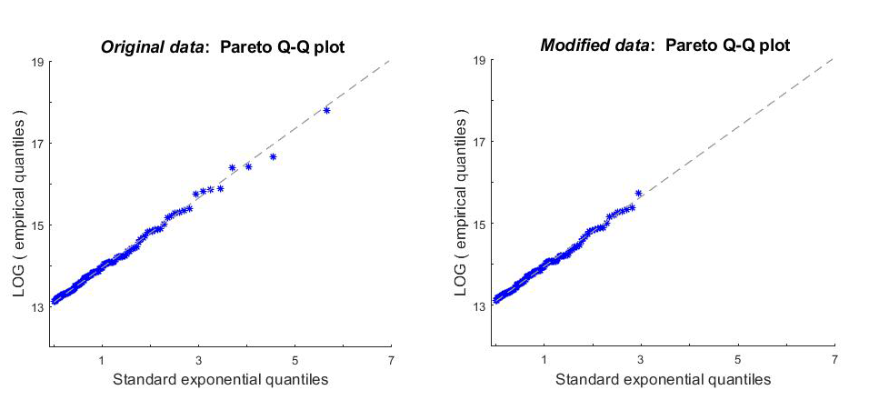
Since no information is given for damages of less than 500,000 nok and there is no policy limit and no coinsurance, the random variable that generated the data is related to payment $Y$—i.e., it is $Y+d$ with $c=1$, $d=500,000$, and $u=\infty$. Moreover, as is evident from Table 5.1, the data are right-skewed and heavy-tailed suggesting that Pareto I, with CDF (4.1) and QF (4.3), might be an appropriate model in this case. To see how right-censoring changes the estimates of $\alpha$, model fits, and ultimately premium estimates for a layer, we consider two data scenarios: original data ($c=1$, $d=500,000$, $u=\infty$) and modified data ($c=1$, $d=500,000$, $u=7,000,000$).

Further, we fit Pareto I$\; (x_0, \alpha)$ under the original and modified data scenarios. Preliminary diagnostics—the quantile-quantile plots (Q-Q plots) presented in Figure 5.1—strongly suggest that the Pareto I assumption is reasonable. Note that the plots are parameter-free. That is, since Pareto I is a log-location-scale family, its Q-Q plot can be constructed without first estimating model parameters. Note also that only actual data can be used in these plots (i.e., no observations $u = 7,000,000$ under the modified data scenario).

5.2. Model estimation and validation

To compute parameter estimates $\widehat{\alpha}$, we use the following formulas: (4.4) for MLE, (4.9) for $T$, and (4.14) for $W$. To match the specifications of the fire claims data (denoted $l_{1}, \ldots, l_{142}$), in (4.4) $c=1$ and $y_i+d$ is replaced with $l_i$; and in (4.9) and (4.14), function $h_Y$ is now defined as $h_Y(l_i) = \log (l_i/d)$. Specifically, for modified data ($d=0.5 \times 10^6$, $u=7 \times 10^6$, claims $l_1, \ldots, l_n$, $n=142$), MLE is given by

$$\small{\widehat{\alpha}_{\small\text{MLE}} = \frac{\sum_{i=1}^{n} \large\mathbf{1}\normalsize \{ d < l_i < u \}} {\sum_{i=1}^{n} \log ( l_i/d ) \large\mathbf{1}\normalsize \{ d < l_i < u \} + \log (u/d) \sum_{i=1}^{n} \large\mathbf{1}\normalsize \{ l_i = u \}}},$$

and for original data ($d=0.5 \times 10^6$, $u=\infty$, claims $l_1, \ldots, l_{n}$, $n=142$), it becomes $\widehat{\alpha}_{\small\text{MLE}} = \frac{n}{\sum_{i=1}^{n} \log ( l_i/d )}.$ Computational formulas for the $T$- and $W$-estimators remain the same for both data scenarios:

$$\begin{aligned}\widehat{\alpha}_{\small\text{T}} &= \frac{(1-a) (1 - \log (1-a)) - b (1 - \log b)}{(1-a-b) \, \widehat{T}_{1(y)}} \\& \mbox{and}\qquad \widehat{\alpha}_{\small\text{W}} = \frac{1-a-b- \log (1-a)}{\widehat{W}_{1(y)}},\end{aligned}$$

where $\widehat{T}_{1(y)} = (n-m_{n}-m_{n}^*)^{-1} \sum_{i = m_{n} + 1}^{n - m_{n}^*} \log( l_i / d)$ and

$$\begin{aligned}\widehat{W}_{1(y)} =&\ n^{-1} \Big[ m_{n} \log{\big( l_{m_{n}+1} / d \big)} \\&+ \sum_{i=m_{n}+1}^{n-m_{n}^{*}}\log{\big( l_{i}/ d \big)} + m_{n}^{*}\log{\big( l_{n-m_{n}^{*}}/ d \big)} \Big],\end{aligned}$$

with several choices of $m_{n} = [n a]$ and $m_{n}^{*} = [n b]$. The corresponding asymptotic distributions are specified by (4.5), (4.11), and (4.15). They are used to construct the 90% confidence intervals for $\alpha$. All computations are summarized in Table 5.2, where goodness-of-fit analysis is also provided; see Klugman, Panjer, and Willmot (2012) for how to perform the Kolmogorov–Smirnov (KS) test for right-censored data (Section 15.4.1) and how to estimate its $p$-value using parametric bootstrapping (Section 19.4.5).

As is evident from Table 5.2, all estimators exhibit excellent goodness-of-fit performance, as one would expect after examining Figure 5.1. Irrespective of the method of estimation, the fitted Pareto I model has a very heavy right tail—i.e., for $1 < \alpha < 2$, all its moments are infinite except the mean. The $T$- and $W$-estimators with $a=b=0$ match the estimates of MLE under the original data scenario. As discussed in Section 4.2, this choice of $a$ and $b$, however, would be inappropriate when data are censored at $u = 7,000,000$, which corresponds to about 4.9% of censoring. Clearly, this level of censoring has no effect whatsoever on $T$- and $W$-estimators with $a=b=0.10$ and $a=0.05, b=0.15$, which demonstrates their robustness. The MLE, on the other hand, is affected by censoring. While the change in its estimated values of $\alpha$ and the corresponding confidence intervals seems minimal (less than 2%), it gets magnified when applied to calculation of premiums, as will be shown next.

5.3. Contract pricing

Let us consider the estimation of the loss severity component of the pure premium for an insurance benefit ($B$) that equals the amount by which a fire loss damage ($L$) exceeds 7 million nok with a maximum benefit of 28 million nok. That is,

$$B = \begin{cases} 0, & \mbox{if} ~~ L \leq d^*; \\[0.25ex] L-d^*, & \mbox {if} ~~ d^* < L \leq u^*; \\[0.25ex] u^* - d^*, & \mbox {if} ~~ L > u^*, \end{cases}\tag{5.1}$$

and, if $L$ follows the distribution function $F$, we seek

$$\begin{aligned}\varPi [F] & ~=~ \mathbf{E}[B] \\& ~=~ \int_{d^*}^{u^*} (x - d^*) \, dF(x) + (u^* - d^*) [ 1-F(u^*) ] \\& ~=~ \int_{d^*}^{u^*} [ 1 - F(x) ] \, d x,\end{aligned}$$

where $d^* = 7 \cdot 10^6$ and $u^* = 35 \cdot 10^6$. (In U.S. dollars, this roughly corresponds to the layer from 1 to 5 million.) We will present premium estimates for two versions of $L$: observed loss (corresponds to $L \sim \mbox{Pareto I} \; (d=5 \cdot 10^5, \alpha)$) and ground-up loss (corresponds to $L \sim \mbox{Pareto I} \; (x_0=7 \cdot 10^3, \alpha)$). The second version shows how different the premium is if all—observed and unobserved—data were available. It also facilitates evaluation of various loss variable characteristics; for example, if one switches from a priority of 500,000 to 250,000, the change in loss elimination ratio could be estimated, but such computations are impossible under the first version of $L$.

Now, straightforward derivations yield the following expression for $\varPi [F]$:

$$\begin{aligned} \varPi [F] ~=~&\ C \times \frac{(u^*/C)^{1-\alpha} - (d^*/C)^{1-\alpha}}{1-\alpha},\\& \qquad \alpha \ne 1,\end{aligned}\tag{5.2}$$

where $C = d$ (for observed loss) or $= x_0$ (for ground-up loss). If $\alpha=1$, then $\varPi [F] = C \log(u^*/d^*)$. To get point estimates $\varPi [\widehat{F}]$, we plug the estimates of $\alpha$ from Table 5.2 into (5.2). To construct interval estimators, we rely on the delta method (see Serfling 1980, Section 3.3), which uses the asymptotic distributions (4.5), (4.11), and (4.15) and transforms $\widehat{\alpha}$ according to (5.2). Thus, we have that $\varPi [\widehat{F}]$ is asymptotically normal with mean $\varPi [F]$ and variance $\mathbf{Var} (\widehat{\alpha}) \times \left( \frac{\partial}{\partial \alpha} \Big[ \varPi [F] \Big] \right)^2,$ where

$$\begin{aligned}\frac{\partial}{\partial \alpha} \Big[ \varPi [F] \Big] =~&\frac{C}{(1-\alpha)^2} \\ &\cdot \Biggl\{ (1-\alpha) \biggl\lbrack \left( \frac{d^*}{C} \right)^{1-\alpha} \log \left( \frac{d^*}{C} \right) \\ &\hspace{10mm}- \left( \frac{u^*}{C} \right)^{1-\alpha} \log \left( \frac{u^*}{C} \right) \biggr\rbrack \\&\hspace{10mm}+ \left( \frac{u^*}{C} \right)^{1-\alpha} - \left( \frac{d^*}{C} \right)^{1-\alpha} \Biggr\}\end{aligned}$$

and $\mathbf{Var} (\widehat{\alpha})$ is taken from (4.5), (4.11), or (4.15). To ensure that the left endpoint of the confidence intervals is positive, we will construct log-transformed intervals, which have the following structure: $\big[ \varPi [\widehat{F}] \cdot K^{-1}; \, \varPi [\widehat{F}] \cdot K \big]$ for $K > 0$. Table 5.3 presents point and 90% log-transformed interval estimates of premiums for observed and ground-up losses under the original and modified data scenarios.

As can be seen from Table 5.3, premiums for the ground-up loss are two orders of magnitude smaller than those for the observed loss. This was expected because the ground-up distribution automatically estimates that the number of losses below 500,000 is large while the observed loss distribution assumes that that number is zero. Further, as the data scenario changes from original to modified, the robust estimates of premiums ($T$ and $W$ with $a=b=0.10$ and $a=0.05$, $b=0.15$) do not change, but those based on MLE increase by 5% (for observed loss) and 11% (for ground-up loss). Finally, note that such MLE-based premium changes occur even though Pareto I fits the data exceptionally well (see Table 5.2). If the model fits were less impressive, the premium swings would be more pronounced.

5.4. Additional illustrations

We mentioned in Section 1 that robust model fits can be achieved by other methods of estimation; one just needs to apply them to trimmed or winsorized data. Since for the Pareto I distribution $T$- and $W$-estimators of $\alpha$ with $a=b=0$ coincide with MLE (see Table 5.2), it is reasonable to expect that left- and/or right-censored MLE should behave like a $W$-estimator with similarly chosen winsorizing proportions. (Such a strategy is sometimes used in data analysis practice to robustify MLE.) In what follows, we investigate how the idea works on Norwegian fire claims.

First of all, the asymptotic properties of MLE as stated in Section 4.1 are valid when the right-censoring threshold $u$ is fixed; hence the probability to exceed it is random. The fixed-thresholds method of moments and some of its variants have been investigated by Poudyal (2021b). The corresponding properties for $T$- and $W$-estimators are established under the complete opposite scenario: data proportions are fixed but thresholds are random. To see what effect this difference has on actual estimates of $\alpha$, we compute MLEs by matching its censoring points with those used for the $T$- and $W$-estimators in Table 5.2. In particular, for $a = b = 0.10$, we have $m_n = m_n^* = [14.2] = 14$, which implies that for observations from $l_{15} = 0.551 \cdot 10^6$ to $l_{128} = 3.289 \cdot 10^6$ their actual values are included in the computation of $\widehat{\alpha}_{\small\text{W}}$, and for the remaining ones the minimum and maximum of actual observations are used, i.e., $l_1 = \cdots = l_{14} = 0.551 \cdot 10^6$ and $l_{129} = \cdots = l_{142} = 3.289 \cdot 10^6$. When computing the censored MLE, this kind of effect on data can be achieved by choosing the left- and right-censoring levels $\widetilde{d}$ and $\widetilde{u}$ as follows: $\widetilde{d} = 0.551 \cdot 10^6$ and $\widetilde{u} = 3.289 \cdot 10^6$. Likewise, for $a = 0.05$ and $b = 0.15$, we have $m_n = [7.1] = 7$ and $m_n^* = [21.3] = 21$ and arrive at $\widetilde{d} = 0.530 \cdot 10^6$ and $\widetilde{u} = 2.497 \cdot 10^6$. Note that $\widetilde{d}$ and $\widetilde{u}$ are not fixed, which is required for derivations of asymptotic properties, but rather they are estimated threshold levels. Rigorous theoretical treatment of MLEs with estimated threshold levels is beyond the scope of the current paper and thus is deferred to future research projects. For illustrative purposes, however, we can assume that the threshold levels $\widetilde{d}$ and $\widetilde{u}$ are fixed and apply the methodology of Section 4.1.

Due to the left-truncation of Norwegian fire claims at $d = 500,000$ and additional left- and right-censoring at $\widetilde{d}$ ($\widetilde{d} > d$) and $\widetilde{u}$, respectively, we are fitting Pareto I$\; (d, \alpha)$ to payment $Z$ data. Given these modifications, $\widehat{\widehat{\alpha}}_{\small\text{MLE}}$ (censored at $\widetilde{d}$ and $\widetilde{u}$) is found by maximizing (4.6) of the following form:

$$\begin{aligned} &{\cal{L}}_{P_Z} \big( \alpha \, \big| \, l_1, \ldots, l_n \big) \\ &\ = \log \big[ 1 - (d/\widetilde{d})^{\alpha} \big] \sum_{i=1}^n \large\mathbf{1}\normalsize \{ l_i = \widetilde{d} \} \\& \quad \ +~ \alpha \log (d/\widetilde{u}) \sum_{i=1}^n \large\mathbf{1}\normalsize \{ l_i = \widetilde{u} \} \\& \quad \ + ~ \sum_{i=1}^n \big[ \log \left( \alpha/d \right) - (\alpha+1) \log \left( l_i/d \right) \big] \large\mathbf{1}\normalsize \{ \widetilde{d} < l_i < \widetilde{u} \}. \qquad ~\end{aligned}$$

Similarly, the asymptotic distribution (4.7) should be of the following form:

$$\begin{align} \widehat{\widehat{\alpha}}_{\small\text{MLE}} ~~is~~ \hspace{34mm} & \\ {\cal{AN}} \Bigg( \alpha, \, \frac{\alpha^2}{n} \, \Bigg[ \frac{\left(\frac{d}{\widetilde{d}}\right)^{\alpha}}{1-\left(\frac{d}{\widetilde{d}}\right)^{\alpha}} \log^2 \left[ \left(\frac{d}{\widetilde{d}}\right)^{\alpha} \right]& \\ + \left(\frac{d}{\widetilde{d}}\right)^{\alpha} - \left(\frac{d}{\widetilde{u}}\right)^{\alpha} \Biggr]^{-1} \Biggr).& \end{align}$$

Numerical implementation of these formulas is provided in Table 5.4, where we compare censored MLEs with $W$ estimators based on such $a$ and $b$ that act on data the same way as MLEs. It is clear from the table that censored MLEs do achieve the same degree of robustness as the corresponding $W$-estimators. Moreover, the point and interval estimates produced by these two methods are very close but not identical. Finally, it should be emphasized once again that the MLE-based intervals are constructed using the assumed asymptotic distribution that is not proven and may be incorrect.

6. Concluding remarks

In the paper, we developed the methods of trimmed (called $T$) and winsorized (called $W$) moments for robust estimation of claim severity models that are affected by deductibles, policy limits, and coinsurance. We provided the definitions and asymptotic properties of those estimators for various data scenarios, including complete, truncated, and censored data, and two types of insurance payments. Further, we derived specific definitions and explicit asymptotic distributions of the maximum likelihood, $T$-, and $W$-estimators for insurance payments when the loss variable follows a single-parameter Pareto distribution. Those analytic examples clearly show that $T$- and $W$-estimators sacrifice little efficiency with respect to MLE but are robust and have explicit formulas (whereas MLE requires numerical optimization; see Section 4.1.2). These are highly desirable properties in practice. Finally, we illustrated the practical performance of the estimators under consideration using the well-known Norwegian fire claims data.

The research presented in the paper invites follow-up studies in several directions. For example, the most obvious direction would be to study small-sample properties of the estimators (for Pareto $\alpha$) using simulations. A second direction might be to derive specific formulas and investigate the estimators’ efficiency properties for other loss models such as lognormal, gamma, log-logistic, folded-$t$, and GB2 distributions. A third avenue might be to consider robust estimation based on different influence functions such as Hampel’s redescending or Tukey’s biweight (bisquare) functions. A fourth line of inquiry could be to compare practical performance of our models’ robustness with that based on model distance and entropy. Note that the latter approach derives the worst-case risk measurements, relative to measurements from a baseline model, and has been used by authors in the actuarial literature (e.g., Blanchet et al. 2019) as well as in the financial risk management literature (see, e.g., Alexander and Sarabia 2012; Glasserman and Xu 2014). Fifth, it would also be of interest to see how well future insurance claims can be predicted using the robust parametric approach of this paper versus more general predictive techniques that are designed to incorporate model uncertainty (see, e.g., Liang Hong and Martin 2017; L. Hong, Kuffner, and Martin 2018).

Finally, to conclude the paper, we briefly discuss how our methodology based on $T$- and $W$-estimators could be extended to applications involving regression with heavy-tailed errors (and potentially incomplete data) and aggregate losses. These are recent and active areas of applied research in insurance (see, e.g., Shi 2014; Shi and Zhao 2020; Delong, Lindholm, and Wüthrich 2021). First of all, the specific examples we present in the paper demonstrate that $T$- and $W$-estimators are well suited for robust fitting of heavy-tailed distributions (e.g., Pareto I) when data are affected by deductibles and policy limits. Second, the regression framework is a major generalization of the underlying assumptions. In this context, several useful results are derived by Lien and Balakrishnan (2005, 2021). Motivated by the problems originating in accounting, those authors investigated the effects on parameter estimates (of a standard regression model) when the covariate data are first cleaned by applying symmetric trimming or winsorization. Those papers surely offer a good start for finding robust estimators of regression parameters, but to make $T$- and $W$-estimators work with heavy-tailed errors, one would have to apply trimming and/or winsorizing to the covariates and the response variable. Third, the aggregate losses are modeled using compound distributions. The severity part of the compound model could be handled directly with $T$- and $W$-estimators. However, at this time, it remains unclear how to modify these estimators to fit the frequency part of the model. This line of investigation is deferred to future research projects.

---

Acknowledgments

The authors are very appreciative of valuable insights and useful comments provided by editor-in-chief Dr. Peng Shi and an anonymous referee that helped to substantially improve the paper. Also, much of the work was completed while the first author was a PhD student in the Department of Mathematical Sciences at the University of Wisconsin–Milwaukee.