1. Introduction

For many years, actuaries have been directed to “consider the credibility assigned to [historical insurance and non-insurance] data” in trend selection (ASB 2009, 7). Credibility considerations are reiterated in the proposed Actuarial Standards of Practice (ASOP) governing the setting of assumptions (ASB 2020). Despite these common-sense articulations of principle, relatively few techniques have been developed in the literature demonstrating how the actuary should achieve this goal. Moreover, existing techniques do not always easily account for all the relevant features impacting trend estimation.

This paper presents a simulation-based model to explicitly account for factors relevant to the estimation of underlying trend. Reflecting important factors such as claim counts, policy limits, or line of business will improve estimates of trend and the distribution of this estimate. The framework presented here immediately lends itself to a Bayesian approach to better incorporate other relevant industry and economic data. External data can help establish the initial set of trend assumptions and prior weights to be used in the model. The simulation results are used to estimate the likelihood of the observed history. By applying Bayes’ theorem, the model provides a credibility-weighted estimate of trend and provides posterior weights applicable to the prior trend set. The posterior view of alternate trend assumptions can be used in capital modeling, sensitivity analysis, or other endeavors in which one must account for parameter uncertainty.

Section 2 presents a partial review of relevant literature addressing the topics of trend credibility, data considerations, and parameter uncertainty. Section 3 outlines the details of the model and highlights the benefits of the framework. Section 4 applies the model to several realistic examples. Section 5 concludes with observations and commentary on trend and the selection of priors.

2. Background literature

Venter (1986) outlines how to use the relative goodness of fit of a trend line alongside a classic square root rule to establish confidence intervals within a desired level of precision. Hachemeister (1975) tackles the problem of state versus countrywide trend parameters using classical generalized least squares, while drawing an analogy between the credibility-weighted slope parameters and the Bühlmann-Straub model. Dickmann and Merz (2001) review ordinary least squares and discuss important data considerations and potential remediation measures, although they do not specifically address credibility. Venter and Sahasrabuddhe (2015) demonstrate the statistical properties of common regression procedures and outline the parameter uncertainty associated therein. Schmid, Laws, and Montero (2013) demonstrate a Bayesian trend selection method for the National Council on Compensation Insurance’s aggregate ratemaking, utilizing a categorical distribution and a Dirichlet prior. This model is used to develop posterior weights to apply to different lengths of experience windows in the trend selection process.

3. Model outline

The three main components of the model are observed data (a trend study), a simulation engine (incorporating benchmark severity or frequency distributions), and a set of “prior” ground-up trends. These three components help address the question, “How likely is it to see the observed trend value if a prior trend is the true parameter value?” Calculating this likelihood allows for the subsequent application of Bayes’ theorem. With this calculation, the model develops a credibility-weighted estimate of constant ground-up trend.

Observed data in this model are treated with “standard” techniques, the output of which are referred to throughout this paper as a “trend study.” Specifically, standard techniques are assumed to use an average metric per year (severity or frequency) as well as exponential regression. Ratemaking papers (e.g., Werner and Modlin 2016, 110–12) outline exponential regression, and Venter and Sahasrabuddhe (2015) outline the associated statistical properties.

To summarize the approach, a severity study may use the following relationship to specify the relationship between severity (X) and time (t):

$$Y_{i} = ln(X_{i})\ = \ \beta_{0} + \beta_{1}t_{i} + \varepsilon_{i}$$

Constant annual trend (subsequently referred to as $O^{*}$) is then estimated as

$$O^{*}\ = \ e^{\beta_{1}}\ - \ 1$$

In practice, $O^{*}$ reflects both the true underlying trend as well as noise from sampling. If error terms are normally distributed, the scaled residuals of $\beta_{1}$ follow a Student’s t-distribution, and confidence intervals may be calculated (Venter and Sahasrabuddhe 2015). However, with annualized aggregate data, the confidence interval may not converge quickly. Furthermore, insurance data may violate the normality assumption (particularly for cases with low claim volumes). With these considerations in mind, there are valid concerns about distributions derived from the statistical properties of least squares regression.

This model uses simulation to estimate the distribution of $O^{*}$. Simulation allows for greater precision and flexibility than the aggregated data used in standard trend studies. Considerations relevant to trend analysis, such as the line of business, claim counts, policy limits, policy limit trending, and attachment points, can all be incorporated into a simulation model. To the extent that these factors may cause $O^{*}$ to differ from the ground-up trend, simulated results will reflect these distortions. Under traditional regression fits, the above considerations are important only to the extent that they impart stability to the goodness of fit (Venter 1986). Useful information is omitted in the standard approach, and stability (or lack thereof) may be a result of the sample. The distribution of trend parameter estimates will differ if the history comprises 25 claims per year versus 250. Unsurprisingly, the volatility of results and parameter estimates for a severity study will differ between a nonstandard auto book with $30,000 policy limits and a products liability book offering $2,000,000 limits. Simulating claim severity directly also incorporates the rich data set underlying benchmark severity distributions by line of business.^[1] One final benefit is that a simulation can produce confidence intervals for an observed trend with only two years of data. The Student’s t-distribution is not defined in this situation, but some distribution around the observed value still exists. Before proceeding, it should be noted that the degree of complexity built into the simulation model should relate to the intended purpose of the model and to the data at hand.

The ground-up prior trends are the final necessary element and represent possible values of the true trend parameter. The prior trends are the mechanism by which this model incorporates industry or other economic data into the analysis. The prior trends are an input to the simulation model—they are treated as the true parameter value when testing how likely it is to see $O^{*}$. The prior weights should reflect the analyst’s belief that the prior value reflects the true parameter. In practice, it is advisable that the high and low points exceed the maximum expected range and that the weighted-average prior reflect the best guess of the true value.

While this model may be applied to either frequency or severity trends, the rest of this paper focuses on severity trends. The remaining elements of the approach and an outline of the Bayesian calculation are specified as follows. Elements with an i index represent different years in the history. The model detrends limits, attachments, and the severity distribution by the length of time between the prospective period and the historical year, making these parameters a function of time.

As presented here, the detrending of the severity distribution assumes that losses of all sizes are affected proportionally. This preserves the coefficient of variation (CV) of the distribution, while the mean is rescaled. Thus, for year i and prior trend k, the relationship to the original severity distribution is as follows:

$${P(X}_{k,i} \leq x) = P\left( X \leq {x \cdot \left( 1 + p_{k} \right)}^{i} \right)\tag{3.1}$$

Detrending the layer limit and attachment by $m$ results in the following for year i:

$$\left( {Lim}_{i} = \frac{Lim}{{(1 + m)}^{i}} \right)\tag{3.2.1}$$

$$\left( {Att}_{i} = \frac{Att}{{(1 + m)}^{i}} \right)\tag{3.2.2}$$

Limits, attachments, and the detrending factor $m$ all impact the observed layered trend, which may not match the ground-up trend. Ideally, $m$ should match the ground-up trend factor. In practice, the ground-up trend factor may not be known, or the analyst may not have access to the original data to alter this factor. Therefore, these three factors are necessary inputs to the model.

This model assumes that trend studies have utilized only claims greater than the layer attachment; therefore, layered claim amounts for year i are as follows:

$$\begin{align} {x}_{i} &\in\left({Att}_{i}, \infty\right] \\ {Loss}_{i}=\bigl\{ {x}-\text{Att}_{i}&, \ \ \ \ \text{Att}_{i}<{x}<\operatorname{Lim}_{i}+\text{Att}_{i} \\ \operatorname{Lim}_{i}&, \ \ \ \ {x} \geq \operatorname{Lim}_{i}+\text{Att}_{i}\bigr. \tag{3.3} \end{align}$$

The loss counts by year are simulated from the commensurate severity distributions by year, and the average severity is recorded. From this point, the model proceeds according to the standard regression-based methods to estimate the exponential trend. This approach is repeated across all prior trends and the desired number of simulations, such that the output matrix is

$$\left(\begin{array}{ccc} \beta_{p_1, 1} & \cdots & \beta_{p_k, 1} \\ \vdots & \ddots & \vdots \\ \beta_{p_1, j} & \cdots & \beta_{p_k, j} \end{array}\right) \tag{3.4}$$

Each column of the output matrix provides an estimate of the distribution of the trend parameter, conditional on prior trend k.

The final element of the model incorporates the prior trend weights ($w_{k}$) and performs the calculations for a Bayesian credibility–weighted estimate. A simulated $\beta_{p_{k},j}$ is considered a “match” in the likelihood calculation ($L_{k}$) when the value is within $(O^{*} \pm \varepsilon)$. The posterior weight ($w_{k}^{*}$) and credibility-weighted trend ($\widehat{t}$) are calculated by

$$w_{k}^{*} = \frac{w_{k}*L_{k}}{\sum_{k \in K}^{}{w_{k}*L}_{k}}\tag{3.5}$$

$$\widehat{t} = \sum_{k \in K}^{}{w_{k}^{*}*p_{k}}\tag{3.6}$$

The examples presented in Section 4 will illustrate that this model is more reliable and robust than traditional least squares for situations in which the required underlying assumptions are mildly or severely violated.

4. Application to realistic scenarios

For each of the hypothetical scenarios in Section 4, this paper will present the key inputs to the model along with a discussion of observations and the results. Sections 4.2 through 4.4 present cases in which data limitations and considerations would reasonably require judgment as to the credibility of the trend study results.

4.1. Large data set, minimal distorting factors

The first example presents an “ideal” scenario for performing a trend study. Starting with this example serves two purposes. First, it’s necessary to demonstrate that a more complex model is consistent with standard techniques for an ideal scenario with sizable claims volume. Second, this example will allow for a comparison to the results of a trend analysis in which distorting factors are present. Table 1 presents the key model inputs as well as the results from the analysis.

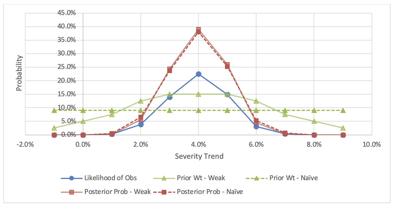
The Bayesian credibility–weighted trend in Table 1 matches the observed value from a study performed using standard techniques. The prior weights in Table 1 are weakly informative and imply an expected trend of 4.0%. However, even a naïve (uniform-weight) prior produces a credibility-weighted estimate of 4.0%. A comparison of these two prior regimes is shown in Figure 1. Naturally, for cases in which the actuary makes use of an informed prior, it is possible to move the credibility-weighted estimate away from the observed value (Gelman 2007). The benefit of this model is that it makes this type of decision explicit and transparent.

Figure 1.Comparison of weak and uniform priors

Before proceeding, a few observations are in order. First, some readers may have noted that the “Average Simulated Trend” in Table 1 does not match the corresponding “Prior Trend” in some cases. This discrepancy is primarily attributable to a mismatch between the “Prior Trend” and the “Trend Applied to Limit and Attachment” $(m)$. When a layer is trended at a different amount than the actual value, this mismatch impacts the measured trend value.^[2] This concept is explored further in Section 4.2.

Second, it is interesting to trace the main elements of the model as they relate to the uncertainty of the true trend factor. The (weak) prior trends are an input and have a central 95th percentile range of [0.0%, 8.0%], reflecting high uncertainty. Observing a 4.0% trend from the data provides information to narrow this range, but the magnitude depends on the simulated distribution. The central 95th percentile of the average simulated trend is roughly 3.5% wide, representing the statistical noise inherent in this scenario.^[3] After evaluating the likelihood of the observed value, the posterior has a central 95th percentile range of [2.0%, 6.0%].^[4] The posterior predictive distribution is also easily derived from the output of this model. The posterior predictive distribution for the weak prior is shown in Figure 2. The posterior predictive distribution has thicker tails than the posterior, as it reflects both the uncertainty of the true trend value and the natural deviation from true values arising from sampling. In the example below, the central 95th percentile for the posterior predictive distribution expands about a point to [1.65%, 6.45%].

Figure 2.Posterior predictive distribution versus weak posterior probability

4.2. Large data set, distorting factors present

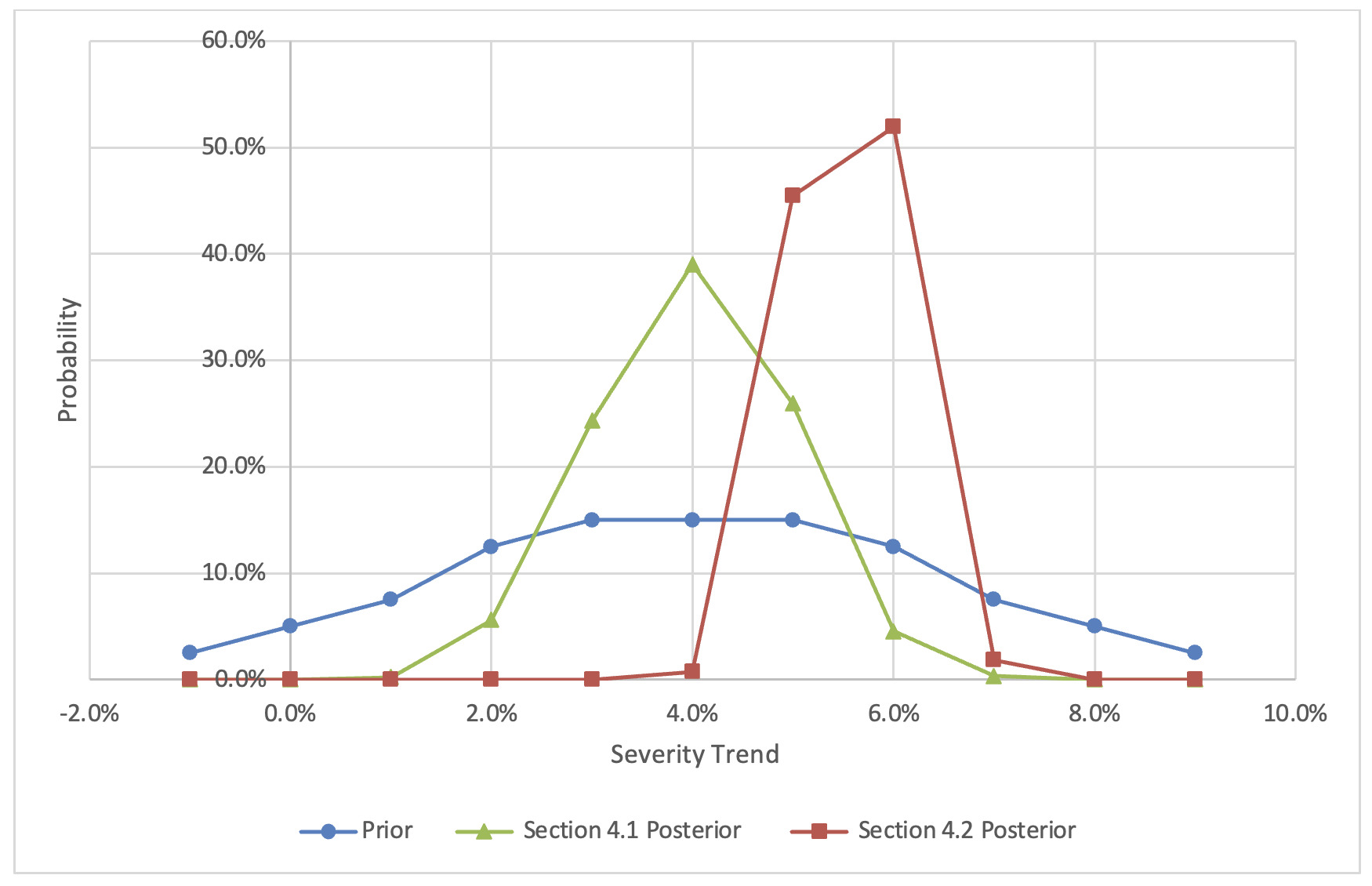
In this section, the example from Section 4.1 is reexamined with a few important modifications. The trend study in this scenario uses a layer capped at $100,000, and a 0.0% trend is applied to this layer.^[5] Other assumptions, including the (ground-up) prior trends and weights, are unchanged. Although this study is not ideally suited to directly estimating the ground-up trend, the following discussion shows that this study can certainly inform such an estimate. A scenario like this could occur when analysts face data limitations or are in the position of relying on studies performed by a third party. In the presence of positive inflation, more losses will be capped by the layer over time. Since these losses cannot inflate, they serve as ballast and push the observed layer trend toward 0.0%. Furthermore, it should be apparent that there are compounding effects between the layer trend and the layer amount, as the layer amount influences the portion of losses that are capped. Due to these distorting factors, observing a 4.0% trend has a markedly different interpretation than it did in Section 4.1. The Bayesian credibility–weighted trend increases to 5.55%, reflecting the tendency for the observed trend to understate the ground-up trend under these circumstances. It is valuable to have techniques to recover the ground-up trend in order to make comparisons with other sources and to have a trend assumption that can be used for different layers. Table 2 shows the updated analysis and input parameters, while Figure 3 compares the posterior probabilities for the “weak” prior under the two scenarios in Sections 4.1 and 4.2.

Figure 3.Comparison of scenarios in Sections 4.1 and 4.2, using “weak” prior

4.3 Changing claims volume over time

It is fairly common to encounter data in which the volume of claims has changed over time. Outside of ad hoc approaches, such as removing years with limited volume, most standard techniques do not account for this factor in the determination of trends. The following example presents the case of a small, but growing, book. The earliest year of the trend study had 75 claims, with the number of claims increasing by 25 per year over an 11-year window.^[6] The following discussion will illustrate how standard regression assumptions are violated and how this violation leads to biased estimates and greater uncertainty.

Note that the “average simulated trend” in Table 3 consistently exceeds the “a priori trend” used in the simulations. What explains this phenomenon? While the average severity is an unbiased measure, the skew and kurtosis depend on the number of observations within the data. Standard trend fitting procedures use the average measured severity per year; when counts differ over time, the assumptions of homoscedasticity and normality are violated. Figure 4 compares the distribution of the average severity statistic at the beginning and end of the experience window for the scenario outlined in Table 3.

Figure 4.Comparing distribution of severity statistic

In the case of low claims volume with increasing claim counts, it is more likely to draw a sample below the mean in the early portion of the history, while samples at the end of the history are more likely to be closer to the mean. Similarly, in the case of decreasing claim counts, the measured trend will tend to understate the true parameter. In the presence of differing claim counts, the shape of the sampling distribution for the mean severity is not the same, a situation that can lead to bias in trend estimates.^[7] Compared with stable books of equivalent volume, this set of circumstances also increases the width of the average simulated trend.^[8]

To conclude this section, observe the manner in which the model adjusts for the dynamics at play. The nature of the data is such that observations will be biased (high) on average. For each prior, the average simulated results are higher than the true parameter, reflecting the bias introduced by the data limitations. Due to this bias, the likelihood calculation will increase weights for priors that are lower than the observation and decrease weights on priors that are higher than the observation. Applying Bayes’ theorem gives a credibility-weighted trend estimate that explicitly contemplates distortions introduced by imperfect empirical data.

4.4. Severity trends for excess layers

This section reviews the topic of differing severity trends for excess layers. This issue has salience in the current environment, where discussions of “frequency of severity” are commonplace. As outlined in Section 3, only losses that exceed the attachment point are captured, while the loss amounts are net of the attachment and are capped by policy limits. When $(m)$ is 0.0%, the pattern of claims observed is akin to a measurement of severity on an umbrella book for U.S. casualty business. Other lines of business or geographies may have unique circumstances that differ from this scenario (e.g., U.S. workers compensation generally does not have policy limits) and therefore require different specifications of the model than those shown in this section.

Table 4 outlines the results for an analysis of (nominal) losses in excess of $2 million, capped at $8 million. Two studies are presented, where the sole difference is the trend applied to the limit and attachment $(m)$. The most striking observation from this simulation is that the average simulated trend factor is nearly identical for all prior trends. Furthermore, the average simulated trend is nearly identical to the trend applied to the limit and attachment. Apart from statistical noise, the model indicates that the analyst should expect the observed value to match the trend applied to the limit and attachment within the study, regardless of the true underlying trend. The analysis contains minimal information, and therefore the Bayesian credibility–weighted trend estimate will default back to the weighted average prior trend assumption.

It can be demonstrated that the results in Table 4 are reasonable: previous literature has covered the disconnect between observed excess and ground-up severity trends (Mata and Verheyen 2005; Brazauskas, Jones, and Zitikis 2009; and Brazauskas, Jones, and Zitikis 2014). Starting from the initial mixed exponential parameters and detrending each mean by 4.0% per year (“trend applied to mean severity”) yields the layer severity results shown in Table 5. For comparison, an equivalent analysis for a lognormal distribution with the equivalent ground-up mean and CV is provided. While these results depend on the severity distribution and layer, one benefit of a simulation-based model is that such considerations immediately come into play. Table 5 demonstrates that severity plays a minimal role in the leveraged aggregate loss trend one would anticipate in a constant-dollar excess layer.

In summary, establishing trends for excess layers based on empirical data will prove challenging. In the interest of minimizing sampling error, this hypothetical scenario included 100 claims per year. Many large loss data sets will have fewer claims and greater uncertainty. A rich and voluminous large-loss data set might allow for generalized linear models or other sophisticated techniques to more convincingly establish differing trends. Analysis reviewing the share of total losses that are “large” (reviewing either the weights of the mixed exponential or the “shape” of the parametric size-of-loss curves over time) may offer insight into severity patterns for large-loss activity.

5. Conclusions and observations

The final section of this paper briefly explores prior selection, the purpose of trend studies, and parameter uncertainty.

There are numerous cases in which actuaries are faced with less than ideal or fully credible data. As demonstrated in Section 4, these imperfections can distort empirically calculated trends. If empirical data are less reliable, this uncertainty heightens the importance of developing appropriate prior distributions. The selection of priors is the analogue to the actuarial judgment invoked in previous literature and discussions. Two reasonable options for priors are presented here, but others are certainly possible. For cases in which industry data are sparse and highly uncertain, a review of economic indices (e.g., the Consumer Price Index for medical care, wages, property values, etc.) could be appropriate. Given concerns that insurance trends might differ from economic indices, a weak prior spread across a wide range of values can be used. Alternatively, for cases in which insurance industry data are more suitable, one might use the known statistical properties of the slope coefficient for exponential regression to inform the prior values and weights. Some caution is warranted with this approach, as it is not guaranteed that the true value lies inside the confidence interval built around the parameter. In either case, should the endpoints of the prior range have meaningful likelihood, it is prudent to reexamine the prior selection.

The actuary must keep in mind the intended purpose of the trend study (ASAB 2009, 2020). Fits to capped data, which will be applied to equivalently capped data prospectively, have different implications than attempts to use the analysis for projects that require the full underlying severity trend. Small data sets with differing claim counts over time may produce trend estimates that are not well suited to trend historical results and may not offer a realistic picture of prospective trends. The analysis in Section 4.4 suggests that standard approaches are frequently ill suited to the purpose of examining excess layer trends. For these scenarios and others, this model offers a statistically justifiable framework to understand the implications of imperfect data and adjust the process accordingly.

The posterior probabilities of different trend assumptions can be taken from this model for use in sensitivity testing and capital modeling. Naturally, there are additional sources of uncertainty beyond those considered within this model. For instance, the loss development factors used in the severity study could have uncertainty around them, as could the severity distribution itself. Clark (2016) and Barnett (2020) present Bayesian techniques to develop posterior weights for development and severity curve selection, respectively. Theoretically, one could incorporate additional sources of uncertainty, but that is outside the scope of this paper. Nonetheless, the author hopes practitioners find that this model offers a useful approach to address one major source of parameter uncertainty in a key assumption in actuarial work.

Acknowledgments

The author thanks Joe Schreier, Stephen Dupon, Dave Clark, and anonymous reviewers for their thoughtful commentary and feedback.