On a Class of Multivariate Mixtures of Gamma Distributions: Actuarial Applications and Estimation Via Stochastic Gradient Methods

1. Introduction

Distributional theory occupies a central place in actuarial research. An extensive literature has been devoted to modeling insurance costs and/or losses using probability distributions. It is fair to state that the problem is relatively more manageable if modeling univariate loss data is encountered. A plethora of distributional models suitable for actuarial applications have been developed; we refer to the monograph (Bahnemann 2015) published by the Casualty Association of Actuaries for a comprehensive summary of univariate parametric distributions commonly used by actuaries.

When insurance losses arise from multiple business lines (BLs) and need to be considered jointly, the modeling task becomes considerably more involved. As one would suspect, the “jungle” of nonnormality in the multivariate setting is not easily tamed. Whether the two-steps copula approach (e.g., Hua and Joe 2017; Hua 2017; Su and Hua 2017) or the more natural stochastic representation approach (e.g., Sarabia et al. 2018, 2016; Kung, Liu, and Wang 2021; Su and Furman 2016, 2017) is pursued to formulate the desired multivariate distribution, the trade-off between flexibility and tractability is often an issue. For the former approach, the resulting multivariate model generally does not possess a workable form and hence must be implemented numerically for actuarial applications. For the latter approach, a major drawback is the lack of flexibility to amalgamate with the suitable marginal distributions, which can have different shapes.

Ideally, a useful multivariate distribution for actuarial applications should enjoy the merits of the two aforementioned approaches, being both flexible statistically and tractable analytically. The multivariate mixtures of Erlang with a common scale parameter, first introduced to the actuarial literature by (S. C. K. Lee and Lin 2012), are exactly one such model. Namely, (S. C. K. Lee and Lin 2012) showed that the multivariate Erlang mixtures form a dense class of multivariate continuous distributions over the nonnegative supports, meaning that any positive data can be fitted by this mixture model with arbitrary accuracy. Moreover, such actuarially important quantities as the tail conditional expectation–based risk measure and allocation principle can be conveniently evaluated in explicit forms under the Erlang mixtures. For these reasons, the multivariate Erlang mixtures have been widely advocated as a parsimonious yet versatile density-fitting tool, suitable for a great variety of modeling tasks in the actuarial practice. That said, due to the integer-valued constraint imposed on the associated parameter space, fitting the Erlang mixtures to multivariate data is by no means trivial. The estimation problem was recently studied in several papers, which involve rather complicated applications of the (conditional) expectation-maximization (EM) algorithm (S. C. K. Lee and Lin 2012; Verbelen et al. 2015; Gui, Huang, and Lin 2021).

In this paper, we aim to put forth a class of multivariate mixtures of gamma distributions with heterogeneous scale parameters. Admittedly, from the distribution theory standpoint, the multivariate gamma mixtures model of interest is a somewhat minor generalization of the multivariate Erlang mixtures in that the shape parameters can take any positive real values and the scale parameters can be varied across different marginal distributions. Nevertheless, we argue that the gamma mixtures distribution is more natural to consider due to a handful of technical reasons, thus deserving separate attention. First, removing the integer-valued constraint on the parameter space induces reams of statistical convenience in the model’s estimation. In this paper, instead of using the EM algorithm adopted in the earlier studies of Erlang mixtures, we propose to use stochastic gradient descent (SGD) methods to estimate the gamma mixtures. The proposed estimation procedure is elegant and transparent. It is worth pointing out that under the integer shape parameters constraint, the Erlang mixtures have the conceptual advantage to studying queueing problems (Breuer and Baum 2005; Tijms 1994) and risk theory (Willmot and Lin 2010); however, for general fitting purposes and many other actuarial applications (e.g., risk measurement, aggregation, and capital allocation), such a constraint is not necessary at all. Second, as opposed to the multivariate mixtures of Erlang with a common scale parameter considered in (S. C. K. Lee and Lin 2012), we allow heterogeneous scale parameters across different marginal distributions. As such, on the one hand, the proposed gamma mixtures are more flexible and robust in density fitting than the Erlang mixtures with a common scale parameter, particularly when the marginal distributions of data are in different magnitudes or measurement units. On the other hand, the proposed gamma mixtures satisfy the scale invariance property, which is desirable in many actuarial and statistics applications (Klugman, Panjer, and Willmot 2012). We note that multivariate Erlang mixtures with heterogeneous scale parameters were also considered in (Willmot and Woo 2014), but the authors did not study the estimation of parameters. So our paper also contributes to filling the vacuum.

The rest of this paper will be organized as follows. In Section 2, the multivariate mixtures of gamma distributions are defined formally. We will take the opportunity to document some distributional properties of the model that are important in insurance applications. Although most of these distributional properties can be viewed as elementary generalizations of the results presented in (Willmot and Woo 2014), the routes that we utilize to establish the results are different, and the expressions in our paper are more elegant and computation friendly. The estimation of parameters for the multivariate gamma mixtures is discussed in Section 3, which constitutes another major contribution of this paper. Section 4 exemplifies the applications of the proposed multivariate gamma mixtures based on simulation data and insurance data. Section 5 concludes the paper.

2. Multivariate mixtures of gamma distributions

In (Venturini, Dominici, and Parmigiani 2008), a class of very flexible univariate distributions constructed by gamma shape mixtures was proposed for modeling medical expenditures of high-risk claimants. Let $\nu\in\mathbf{N}$ be a discrete random variable (RV) with probability mass function (PMF), $p_\nu(v):=\mathbf{P}(\nu=v)$ for $v\in\mathbf{R}_+$; the definition of the univariate gamma mixtures in (Venturini, Dominici, and Parmigiani 2008) is given as follows.

Definition 1 (Venturini, Dominici, and Parmigiani 2008). We say that RV $X\in \mathbf{R}_+$ is distributed mixed-gamma (MG) having scale parameter $\theta\in \mathbf{R}_+$ and stochastic shape parameter $\nu$, succinctly $X\sim {\rm MG}(\theta,p_{\nu})$, if its probability density function (PDF) is given by

$$f_X(x)=\sum_{v \in \operatorname{supp}(\nu)} p_\nu(v) \frac{x^{v-1} \theta^{-v}}{\Gamma(v)} e^{-x / \theta}, \quad x \in \mathbf{R}_{+} \tag{1}$$

where the notation “${\rm supp}(\nu)$” denotes the support of RV $\nu$, and $\Gamma(v):=\int_0^{\infty} s^{v-1}e^{-s}ds$ denotes the gamma function.

The subsequent result follows immediately, and its proof is straightforward and thus omitted.

Proposition 1. Assume that $X\sim {\rm MG}(\theta,p_{\nu})$; then the decumulative distribution function (DDF) of $X$ is given by

$$\bar{F}_X(x)=\sum_{v \in \operatorname{supp}(\nu)} p_\nu(v) \frac{\Gamma(v, x / \theta)}{\Gamma(v)}, \quad x \in \mathbf{R}_{+} \tag{2}$$

where $\Gamma(v,x):=\int_x^{\infty} s^{v-1}e^{-s}ds$ denotes the upper incomplete gamma function, $v>0$. Moreover, for any $a>0$,

$$\mathbf{E}\left[X^a\right]=\theta \mathbf{E}[\Gamma(\nu+a) / \Gamma(\nu)] \tag{3}$$

In this paper, we are interested in a multivariate extension of the gamma shape mixtures as per Definition 1 for modeling dependent insurance data. The multivariate extension of interest is inspired by the multivariate Erlang mixtures considered in (Furman, Kye, and Su 2020a; S. C. K. Lee and Lin 2012; Willmot and Woo 2014; Verbelen et al. 2015). Namely, the multivariate gamma mixtures, which we are going to propose next, generalize the just-mentioned Erlang mixtures by allowing for arbitrary nonnegative real-valued shape parameters as well as heterogeneous scale parameters among the marginal distributions. For $d\in \mathbf{N}$, let $\boldsymbol{\nu}=(\nu_1,\ldots,\nu_d)\in \mathbf{R}_+^d$ be a vector of discrete RVs with joint PMF $p_{\boldsymbol{\nu}}(\boldsymbol{v}):=\mathbf{P}(\boldsymbol{\nu}=\boldsymbol{v})$, $\boldsymbol{v}=(v_1,\ldots,v_d)\in \mathbf{R}_+^d$. The RV $\boldsymbol{\nu}$ is used to denote the stochastic shape parameters in the multivariate gamma mixtures.

Definition 2. The RV $\boldsymbol{X}=(X_1,\ldots,X_d)$ is said to be distributed $d$-variate mixtures of gamma ($MG_d$) if the corresponding joint PDF is given by

$$\small{ \begin{align} f_{\boldsymbol{X}}\left(x_1, \ldots, x_d\right)&=\sum_{v \in \operatorname{supp}(\nu)} p_{\boldsymbol{\nu}}(\boldsymbol{v}) \prod_{i=1}^d \frac{x_i^{v_i-1} \theta_i^{-v_i}}{\Gamma\left(v_i\right)} e^{-x_i / \theta_i}, \\ &\quad \left(x_1, \ldots, x_d\right) \in \mathbf{R}_{+}^d, \end{align} } \tag{4}$$

where $\theta_{i}>0$, $i=1,\ldots,d$, are the scale parameters. Succinctly, we write $\boldsymbol{X}\sim {\rm MG}_d(\boldsymbol{\theta},p_{\boldsymbol{\nu}})$ with $\boldsymbol{\theta}=(\theta_1,\ldots,\theta_d)$.

The ${\rm MG}_d$ distribution in Definition 2 generalizes a handful of existing models. In particular, if RV $\boldsymbol{\nu}$ is restricted to be integer valued, then PDF (4) collapses to the Erlang mixtures considered in Furman, Kye, and Su (2020a) and Willmot and Woo (2014). Further, if the coordinates of $\boldsymbol{\theta}$ are identical, then the ${\rm MG}_d$ distribution reduces to the multivariate Erlang mixtures with a common scale parameter (S. C. K. Lee and Lin 2012). Consequently, the ${\rm MG}_d$ distribution preserves the denseness property of the multivariate Erlang mixtures, being capable of approximating any positive data.

The succeeding assertion pertains to a few elementary properties of the ${\rm MG}_d$ distribution. The results are straightforward extensions of Theorem 3 in Furman, Kye, and Su (2020a), so the proofs are omitted.

Proposition 2. Consider $\boldsymbol{X}\sim {\rm MG}_d(\boldsymbol{\theta},p_{\boldsymbol{\nu}})$; then the following assertions hold.

1. The joint Laplace transform that corresponds to RV $\boldsymbol{X}$ is

$$\begin{align} \mathcal{L}\left\{f_{\boldsymbol{X}}\right\}\left(t_1, \ldots, t_n\right)&=P_\nu\left(\frac{1}{1+\theta_1 t_1}, \ldots, \frac{1}{1+\theta_d t_d}\right), \\ &\quad\left(t_1, \ldots, t_d\right) \in \mathbf{R}_{+}^d, \end{align}$$

where $P_{\boldsymbol{\nu}}$ denotes the joint probability generating function of RV $\boldsymbol{\nu}$.

2. The joint higher-order moments of $\boldsymbol{X}$ can be computed via

$$\begin{align} \mathbf{E}\left[X_1^{a_1} \cdots X_d^{a_d}\right]&=\prod_{i=1}^d \theta_i^{a_i} \times \mathbf{E}\left[\prod_{i=1}^d \frac{\Gamma\left(\nu_i+a_i\right)}{\Gamma\left(\nu_i\right)}\right], \\ &\quad\left(a_1, \ldots, a_d\right) \in \mathbf{R}_{+}^d, \end{align}$$

assuming that the expectations exist.

3. The marginal coordinates of $\boldsymbol{X}$ are distributed univariate MG; namely, $X_i\sim {\rm MG}(\theta_i, p_{\nu_i})$, where $p_{\nu_i}$ denotes the $i$-th coordinate marginal PMF of $\boldsymbol{\nu}$, $i=1,\ldots,d$.

Proposition 2 reveals that PDF (4) is conditionally independent given $\boldsymbol{\nu}$ but unconditionally dependent. On the one hand, the conditional independence construction retains the mathematical tractability inherent in the gamma distribution to a great extent. As we will see in the next subsection, many useful actuarial quantities can be derived conveniently in analytical forms under the ${\rm MG}_d$ model. On the other hand, the dependencies of multivariate insurance data can be captured by the mixture structure in the ${\rm MG}_d$ distribution. The next corollary underscores that the ${\rm MG}_d$ distribution can handle independence as well as positive and negative pairwise dependence. Its proof follows from Proposition 2.

Corollary 3. Assume that $\boldsymbol{X}\sim {\rm MG}_d(\boldsymbol{\theta},p_{\boldsymbol{\nu}})$; then the following assertions hold.

1. RV $\boldsymbol{X}$ is independent if and only if coordinates of $\boldsymbol{\nu}$ are independent.

2. Choose $1\leq i\neq j\leq d$, and suppose that $\nu_i,\nu_j\in L^2$; then the Pearson correlation between $X_i$ and $X_j$ can be evaluated via

$$\small{ \operatorname{Corr}\left(X_i, X_j\right)=\operatorname{Corr}\left(\nu_i, \nu_j\right) \frac{\sqrt{\operatorname{Var}\left(\nu_i\right) \operatorname{Var}\left(\nu_j\right)}}{\sqrt{\left(\operatorname{Var}\left(\nu_i\right)+\mathbf{E}\left[\nu_i\right]\right)\left(\operatorname{Var}\left(\nu_j\right)+\mathbf{E}\left[\nu_j\right]\right)}} }$$

Moreover, the sign of ${\rm Corr}(X_i, X_j)$ can be both negative and positive, stipulated by ${\rm Corr}(\nu_i,\nu_j)$, which can attain any value in the interval $[-1,1]$.

Another important property of ${\rm MG}_d$ that we should study next is the aggregate distribution. Namely, let $S_{\boldsymbol{X}}=X_1+\cdots+X_d$, with $\boldsymbol{X}\sim {\rm MG}_d(\boldsymbol{\theta},p_{\boldsymbol{\nu}})$. We now are interested in studying the distribution of $S$. To this end, the following lemma is of auxiliary importance.

Lemma 4 (Corollary 7 in Furman, Kye, and Su 2020a; also see Lemma 1 in Furman and Landsman 2005). Suppose that RVs $Y_1,\ldots,Y_d$ are independently distributed gamma with $Y_i\sim {\rm Ga}(\theta_i,\gamma_i)$, where $\theta_i>0$ and $\gamma_i>0$ are the scale and shape parameters, respectively, $i=1,\ldots,d$. Let $\boldsymbol{\gamma}=(\gamma_1,\ldots,\gamma_d)$, $\boldsymbol{\theta}=(\theta_1,\ldots,\theta_d)$, $\gamma^*=\gamma_1+\cdots+\gamma_d$, and $\theta^*=\bigwedge_{i=1}^d \theta_i$. Then the aggregate RV $S_{\boldsymbol{Y}}=Y_1+\ldots+Y_d$ is distributed ${\rm MG}(\theta^*,p_{\nu^*})$, where ${\nu^*}:={\nu^*}(\boldsymbol{\theta},\boldsymbol{\gamma})\overset{D}{=}\gamma^*+\sum_{i=1}^d N_i$ is the shifted convolution of independent negative binomial RVs, $N_i\sim {\rm NB}(\gamma_i,\theta^*/\theta_i)$, $i=1,\ldots,d$. Here and throughout, “$\overset{D}{=}$” signifies the equality in distribution.

Remark 1. Although the PMF of negative binomial convolution in Lemma 4 does not possess an explicit expression, it still can be evaluated conveniently by Panjer’s recursive method (Panjer 1981). We also refer to Theorem 5 in Furman, Kye, and Su (2020a) for a more peculiar discussion about the recursive method.

The succeeding result follows immediately from Lemma 4, which asserts that the aggregation of ${\rm MG}_d$ RVs is distributed mixed gamma.

Proposition 5. Assume that RV $\boldsymbol{X}\sim {\rm MG}_d(\boldsymbol{\theta},p_{\boldsymbol{\nu}})$, then $S_{\boldsymbol{X}}\sim {\rm MG}(\theta^*,p_{\omega})$, where $\theta^*=\bigwedge_{i=1}^d \theta_i$ and for any $\boldsymbol{v}=(v_1,\ldots,v_d)\in {\rm supp}(\boldsymbol{\nu})$, $v^*=v_1+\cdots+v_d$,

$$\begin{align} p_\omega(x)&=\sum_{\boldsymbol{v} \in \operatorname{supp}(\boldsymbol{\nu})} p_{\boldsymbol{\nu}}(\boldsymbol{v}) \times p_{\nu^*(\boldsymbol{\theta}, \boldsymbol{v})}(x), \\ x&=v^*, v^*+1, v^*+2, \ldots \end{align} \tag{5}$$

with ${\nu^*}:={\nu^*}(\boldsymbol{\theta},\boldsymbol{v})\overset{D}{=}v^*+\sum_{i=1}^d N_i$ is the shifted convolution of independent negative binomial RVs, $N_i\sim {\rm NB}(v_i,\theta^*/\theta_i)$, $i=1,\ldots,d$.

Pioneered by Furman and Landsman (2005), the notion of multivariate size-biased transforms has been shown to furnish a useful computation tool in the study of risk measure and allocation (Ren 2021; Furman, Kye, and Su 2020b; Denuit 2020, 2019). Specifically, let $\boldsymbol{h}=(h_1,\ldots,h_d)\in \{0,1 \}^d$ be a constant vector containing zero or one elements; then the multivariate size-biased variant of a positive RV $\boldsymbol{X}=(X_1,\ldots,X_d)\in\mathbf{R}_+^d$, denoted by $\boldsymbol{X}^{[\boldsymbol{h}]}=(X_1^{[h_1]},\ldots,X_d^{[h_d]})$, is defined via

$$\begin{aligned} \mathbf{P}\big(\boldsymbol{X}^{[\boldsymbol{h}]}\in d\boldsymbol{x}\big)=\frac{x_1^{h_1}\cdots x_d^{h_d}}{{\mathbf E}\big[X_1^{h_1}\cdots X_d^{h_d}\big]}\mathbf{P}(\boldsymbol{X}\in d\boldsymbol{x}). \end{aligned}$$

Next, we show that the class of multivariate gamma mixtures in Definition 2 is closed under size-biased transforms.

Proposition 6. Suppose that $\boldsymbol{X}\sim {\rm MG}_d(\boldsymbol{\theta},p_{\boldsymbol{\nu}})$; then $\boldsymbol{X}^{[\boldsymbol{h}]}\sim {\rm MG}(\boldsymbol{\theta}, p_{\boldsymbol{\nu}^{[\boldsymbol{h}]}+\boldsymbol{h}})$, where $\boldsymbol{\nu}^{[\boldsymbol{h}]}$ is the multivariate size-biased counterpart of $\boldsymbol{\nu}$.

Proof. For $\boldsymbol{x}=(x_1,\ldots,x_d)\in \mathbf{R}_+^d$, the PDF of $\boldsymbol{X}^{[\boldsymbol{h}]}$ can be computed via

$$\small{ \begin{aligned} f_{\boldsymbol{X}[\boldsymbol{h}]}(\boldsymbol{x})&=\frac{x_1^{h_1} \cdots x_d^{h_d}}{\mathbf{E}\left[X_1^{h_1} \cdots X_d^{h_d}\right]} \sum_{\boldsymbol{v} \in \operatorname{supp}(\boldsymbol{\nu})} p_{\boldsymbol{\nu}}(\boldsymbol{v}) \prod_{i=1}^d \frac{x_i^{v_i-1} \theta_i^{-v_i}}{\Gamma\left(v_i\right)} e^{-x_i / \theta_i} \\ & =\sum_{\boldsymbol{v} \in \operatorname{supp}(\boldsymbol{\nu})} \frac{v_1^{h_1} \cdots v_d^{h_d}}{\mathbf{E}\left[\nu_1^{h_1} \cdots \nu_d^{h_d}\right]} p_{\boldsymbol{\nu}}(\boldsymbol{v}) \prod_{i=1}^d \frac{x_i^{\left(v_i+h_i\right)-1} \theta_i^{-\left(v_i+h_i\right)}}{\Gamma\left(v_i+h_i\right)} e^{-x_i / \theta_i} \\ & =\sum_{\boldsymbol{v} \in \operatorname{supp}(\boldsymbol{\nu})} p_{\boldsymbol{\nu}^{[h]}}(\boldsymbol{v}) \prod_{i=1}^d \frac{x_i^{\left(v_i+h_i\right)-1} \theta_i^{-\left(v_i+h_i\right)}}{\Gamma\left(v_i+h_i\right)} e^{-x_i / \theta_i}, \\ \end{aligned} }$$

which yields the desired result.

2.1. Actuarial applications

The discussion hitherto has a strong favor of distribution theory, yet it is remarkably connected to real-world insurance applications. Now let $\boldsymbol{X}=(X_1,\ldots,X_d)\in \mathbf{R}_+^d$ represent a portfolio of dependent losses; a central problem in insurance is to quantify the risks due to the individual component $X_i$, $i=1,\ldots,d,$ as well as the aggregation $S_{\boldsymbol{X}}=\sum_{i=1}^d X_i$. In the context of quantitative risk management, two popular risk measures are Value-at-Risk (VaR) and the conditional tail expectation (CTE). To be specific, let $X>0$ be a risk RV and fix $q\in[0,1)$; the VaR is defined as $$\begin{aligned} x_q:={\mathrm{VaR}}_q(X)=\inf\{x\geq 0: F_{X}(x)\geq q \}, \end{aligned}$$ where $F_X$ denotes the cumulative distribution function (CDF) of $X$, and the CTE risk measure is given by $$\begin{aligned} {\mathrm{CTE}}_q[X]={\mathbf E}[X|X>x_q], \end{aligned}$$ assuming that the expectation exists. We start off by considering the CTE for the univaraite gamma mixtures in Definition 1.

Proposition 7. Suppose that risk RV $X\sim {\rm MG}(\theta,p_{\nu})$; then the CTE of $X$ can be computed via $$\begin{aligned} {\mathrm{CTE}}_q[X]=\frac{{\mathbf E}[X]}{1-q}\, \overline{F}_{X^{[1]}}(x_q),\qquad \mbox{$q\in [0,1)$,} \end{aligned}$$ where $x_q={\mathrm{VaR}}_q(X)$, $X^{[1]}$ denotes the first-order size-biased variant of $X$ and $X^{[1]}\sim {\rm MG}(\theta,p_{\nu^{ [1]}+1})$ according to Proposition 6. The DDF and expectation involved in the CTE formula above can be computed via Equations (2) and (3), respectively.

Proof. The proof is due to the following identity:

$$\begin{align} \operatorname{CTE}_q[X]=\frac{\mathbf{E}\left[X \mathbf{1}\left(X>x_q\right)\right]}{1-q}=\frac{\mathbf{E}[X]}{1-q} \mathbf{E}\left[\mathbf{1}\left(X>x_q\right)\right], \end{align}$$

where $\mathbf{1}(\cdot)$ denotes the indicator function. The desired result is established.

The next assertion spells out the formulas for evaluating the CTE risk measures when dependent risks $\boldsymbol{X}$ are modeled by the multivariate gamma mixtures. The results follow by evoking Propositions 2, 5, 6 and 7.

Proposition 8. Assume that $\boldsymbol{X}=(X_1,\ldots,X_d)\sim {\rm MG}_d(\boldsymbol{\theta},p_{\boldsymbol{\nu}})$, and let $S_{\boldsymbol{X}}=\sum_{i=1}^dX_i$. For $q\in [0,1)$ and $i=1,\ldots,d$, define $x_{i,q}={\mathrm{VaR}}_q(X_i)$ and $s_q={\mathrm{VaR}}_q(S_{\boldsymbol{X}})$. The CTE of the individual risks $X_i$ can be computed via

$$\mathrm{CTE}_q\left[X_i\right]=\frac{\mathbf{E}\left[X_i\right]}{1-q} \bar{F}_{X_i^{[1]}}\left(x_{i, q}\right)$$

where the expectation ${\mathbf E}[X_i]$ can be computed via Equation (3), and the DDF of $X_i^{[1]}\sim {\rm MG}(\theta_i, p_{\nu_i^{[1]}+1})$ can be computed by evoking Proposition 6 and then Equation (2).

Moreover, the CTE of the aggregate risk is computed via

$$\mathrm{CTE}_q\left[S_{\boldsymbol{X}}\right]=\frac{\mathbf{E}\left[S_{\boldsymbol{X}}\right]}{1-q} \bar{F}_{S_{\boldsymbol{X}}^{[1]}}\left(s_q\right), \tag{6}$$

The size-biased counterpart of $S_{\boldsymbol{X}}$ is $S_{\boldsymbol{X}}^{[1]}\sim {\rm MG}(\theta^*, p_{\omega^{[1]}+1})$, where $\theta^*=\bigwedge_{i=1}^d \theta_i$ and the distribution of $\omega$ is specified as per Equation (5).

Remark 2. The aggregate CTE formula (6) in Proposition 8 contains an expectation term and a DDF term. The expectation term ${\mathbf E}[S_{\boldsymbol{X}}]={\mathbf E}[X_1]+\cdots+{\mathbf E}[X_d]$ can be easily evaluated by repeated applications of formula (3) to every marginal distribution. By evoking Proposition 5, the DDF term is computed via

$$\begin{align} \bar{F}_{S_{\boldsymbol{X}}^{[1]}}\left(s_q\right)&=\sum_{k \in \operatorname{supp}(\omega)} p_{\omega^{[1]}}(k+1) \\ &\quad \times \bar{G}\left(s_q ; k+1, \theta^*\right), \end{align}$$

where $\overline{G}(\cdot\,;\,\gamma,\theta)$ denotes the DDF of a gamma distribution with shape parameter $\gamma>0$ and scale parameter $\theta>0$. Note that the support of $\omega$ is unbounded (see Equation (5)), so there is an infinite series involved in the calculation of DDF above. In practical computation, the infinite series must be truncated at a finite point, and we may use the first, say $m\in \mathbf{N}$, terms of the series to approximate the infinite series, where $m$ is such that the desired accuracy is attained. Compared with the aggregate CTE formula derived in (Willmot and Woo 2014) for Erlang mixtures, expression (6) in our paper is more elegant and computation friendly in the sense that a bound for the resulting truncation error can be conveniently found by noticing that DDF $\overline{G}$ must be bounded above by $1$, so the truncation error must be smaller than or equal to one minus the first $m$-terms sum of the weights $p_{\omega^{[1]}+1}(\cdot)$.

The calculation of CTE risk measure plays an pivotal role in determining the economic capital, which however is only a small piece of the encompassing framework of enterprise risk management. Another important component is the notion of economic capital allocation. In this respect, the CTE-based allocation principle is of particular interest, and it is defined as $$\begin{aligned} {\mathrm{CTE}}_q[X_i, S_{\boldsymbol{X}}]:={\mathbf E}\big[X_i\, |\, S_{\boldsymbol{X}}>s_q\big], \qquad q\in[0,1), \end{aligned}$$ where $s_q={\mathrm{VaR}}_q(S_{\boldsymbol{X}})$ is the VaR of aggregate risk $S$, assuming that the expectation exists.

Proposition 9. Suppose that $\boldsymbol{X}\sim {\rm MG}_d(\boldsymbol{\theta},p_{\boldsymbol{\nu}})$; then the CTE allocation rule can be evaluated via

$$\operatorname{CTE}_q\left[X_i, S\right]=\frac{\mathbf{E}\left[X_i\right]}{1-q} \times \bar{F}_{S_{X^{\left[h_i\right]}}}\left(s_q\right), \quad i=1, \ldots, d$$

where $S_{\boldsymbol{X}^{[\boldsymbol{h}_{i}]}}$ denotes the aggregation of $\boldsymbol{X}^{[\boldsymbol{h}_i]}$, which is the multivariate size-biased variant of $\boldsymbol{X}$ with $\boldsymbol{h}_{i}$ being a $d$-dimensional constant vector having the $i$-th element equal to one and zero elsewhere. The DDF of $S_{\boldsymbol{X}^{[\mathbf{h}_{i}]}}$ can be evaluated by evoking Propositions 5 and 6 and Remark 2.

Proof. The proof is similar to that of Proposition 7. We have

$$\begin{align} \mathrm{CTE}_q\left[X_i, S\right]&=\frac{\mathbf{E}\left[X_i \mathbf{1}\left(S_{\boldsymbol{X}}>s_q\right)\right]}{1-q}\\ &=\frac{\mathbf{E}\left[X_i\right]}{1-q} \mathbf{E}\left[\mathbf{1}\left(S_{\boldsymbol{X}^{\left[h_i\right]}}>s_q\right)\right] \end{align}$$

which completes the proof.

3. Parameter estimation: A stochastic gradient decent approach

In the earlier studies of multivariate Erlang mixtures, the EM algorithm was adopted to estimate the parameters (S. C. K. Lee and Lin 2012; Verbelen et al. 2015). Applying the EM algorithm to estimate the ${\rm MG}_d$ distribution may be computationally onerous. To explain the reason, note that the validity of the universal approximation property of ${\rm MG}_d$ requires the number of mixture components, say $m\in \mathbf{N}$, to be sufficiently large. However, $m$ is unknown, so it must be estimated from data. Typically, the estimation procedure starts with a very large number of mixture components first, and later, mixture components with relatively small mixture weights are dropped in order to produce a parsimonious fitted model. Consequently, in each iteration of the EM algorithm for updating the parameter estimates, one has to solve multiple systems of high-dimensional, nonlinear optimizations, which do not possess closed-form solutions. The inherent optimization problems must be solved numerically, but due to the curse of dimensionality, commonly used “black-box” numerical optimizers from commercial statistics software may become inefficient and even unreliable.

In this paper, we are interested in a more computation-friendly alternative to the EM algorithm to fit the proposed ${\rm MG}_d$ distribution to data. In particular, it is desirable that the estimation method (1) can estimate a large number of parameters simultaneously, (2) possesses a transparent algorithm without using “black-box” numerical solvers, (3) is elegant for practicing actuaries to implement, and (4) enables parallel computing for massive insurance data applications. Taking these aspects into consideration, the SGD method, which achieves great successes in the recent machine learning literature, is natural to evoke.

In order to facilitate the subsequent discussion, we find that it is convenient to rewrite the joint PDF of ${\rm MG}_d$ in Equation 4 as

$$\begin{align} f_{\boldsymbol{X}}(\boldsymbol{x} ; \boldsymbol{\alpha}, \boldsymbol{\gamma}, \boldsymbol{\theta})&=\sum_{j=1}^m \alpha_j \prod_{i=1}^d \frac{x_i^{\gamma_{i j}-1} \theta_i^{-\gamma_{i j}}}{\Gamma\left(\gamma_{i j}\right)} e^{-x_i / \theta_i}, \\ \boldsymbol{x}&=\left(x_1, \ldots, x_d\right) \in \mathbf{R}_{+}^d \end{align} \tag{7}$$

such that $\boldsymbol{\gamma}=(\boldsymbol{\gamma}_1,\ldots,\boldsymbol{\gamma}_m)^\top$ with $\boldsymbol{\gamma}_j=(\gamma_{1j},\ldots,\gamma_{dj})$, $j=1,\ldots,m$, collects all possible realizations of the stochastic shape parameters $\boldsymbol{\nu}$, $\boldsymbol{\alpha}=(\alpha_1,\ldots,\alpha_m)\in \mathbf{R}_+^m$ contains the corresponding mixture weights satisfying $\sum_{j=1}^m\alpha_j=1$, and same as the representation in Equation (4), $\boldsymbol{\theta}=(\theta_1,\ldots,\theta_d)\in \mathbf{R}_+^d$ denotes the set of the scale parameters for different marginal distributions.

Consider a collection of $n$ sets of $d$ dimensional data, $\boldsymbol{x}=(\boldsymbol{x}_{1},\ldots,\boldsymbol{x}_{n})^\top$, with $\boldsymbol{x}_k=(x_{1\,k}\,,\ldots,\,x_{d\,k})$, $k=1,\ldots,n$. We aim to approximate the data distribution by ${\rm MG}_d$ for statistical inferences. Thus, the essential task is to derive the maximum likelihood estimators (MLEs) for parameters $\boldsymbol{\Psi}=(\boldsymbol{\alpha},\boldsymbol{\gamma},\boldsymbol{\theta})$, which equivalently minimizes the following negative log-likelihood function:

$$\begin{align} h(\Psi)&=\frac{1}{n} \sum_{k=1}^n h_k(\Psi), \\ \text{where} \ h_k(\Psi)&=-\log f_{\boldsymbol{X}}\left(\boldsymbol{x}_k ; \boldsymbol{\alpha}, \boldsymbol{\gamma}, \boldsymbol{\theta}\right) \end{align} \tag{8}$$

The SGD algorithm finds a (local) minimum of objective function (8) via iterative updates: For $s\in \mathbf{N}$, $\boldsymbol{\Psi}^{(s)}= \boldsymbol{\Psi}^{(s-1)}-\delta_s\, \widehat\nabla h(\boldsymbol{\Psi}^{(s-1)})$, where $\widehat\nabla h(\boldsymbol{\Psi}^{(s-1)})$ denotes the stochastic gradient, which is an unbiased estimation of $\nabla h(\boldsymbol{\Psi}^{(s-1)})$, and to ensure that the algorithm will converge, the learning rate $\delta_s>0$ is chosen such that

$$\begin{aligned} (i)\ \sum_{s=1}^{\infty} \delta_s =\infty;\qquad (ii)\ \sum_{s=1}^{\infty} \delta_s^2 <\infty. \end{aligned}$$

For instance, one may set $\delta_s=s^{-b}$ with $b\in (0,1]$, under which the two above conditions will be satisfied. Regarding the stochastic gradient $\widehat\nabla h(\cdot)$ in the $s$-th interaction step, a simple yet common choice is $\nabla h_{\kappa_s}(\cdot)$, where the index $\kappa_s$ is chosen uniformly at random, with $\mathbf{P}(\kappa_s=k)=1/n$, $k=1,\ldots,n$, corresponding to the gradient of the negative log-likelihood function based on a randomly sampled data point.

Before applying the aforementioned SGD method to estimate the ${\rm MG}_d$ distribution, it is noted that the mixture weights $\boldsymbol{\alpha}$ must reside on a low dimensional manifold $\Omega:=\{\alpha_j>0, \sum_{j=1}^m\alpha_j=1\}$. Directly updating the estimate of $\boldsymbol{\alpha}$ via the conventional SGD will violate this constraint, yielding an invalid estimation result. For this reason, we suggest reparameterizing $\boldsymbol{\alpha}$ by $\boldsymbol{\alpha}^*=(\alpha_1^*,\ldots,\alpha_m^*)$, where $\alpha_j={\exp (\alpha_j^*)}\,/\,{\sum_{l=1}^{m} \exp(\alpha_l^*)}$ for $j=1,\ldots,m$. The proposed reparametrization, which maps $\Omega$ to the whole space $\mathbf{R}^{m}$, conveniently resolves the issue mentioned above.^[1] In a similar vein, we reparametrize $\gamma_{ij}$ and $\theta_i$ via $\gamma^*_{ij}=\log(\gamma_{ij})$ and $\theta_{i}^*=\log(\theta_i)$, $i=1,\ldots,d$, $j=1,\ldots,m$, and update the estimates of $\boldsymbol{\gamma}^*=(\boldsymbol{\gamma}^*_1,\ldots,\boldsymbol{\gamma}^*_m)$ with $\boldsymbol{\gamma}_j^*=(\gamma^*_{1j},\ldots,\gamma^*_{dj})$ and $\boldsymbol{\theta}^*=(\theta_1^*,\ldots,\theta_d^*)$ instead of $\boldsymbol{\gamma}$ and $\boldsymbol{\theta}$ so that the positive constraints on the original shape and scale parameters can be removed.

Further, for brevity, let us define

$$\small{ \begin{aligned} g(\boldsymbol{x};\boldsymbol{\gamma}_j^*,\boldsymbol{\theta}^*) &= \prod_{i=1}^d \frac{1}{\Gamma\big(\exp(\gamma_{ij}^*)\big)}\,\exp\big(-{x_i\, e^{-\theta_i^*}}-\theta_i^*\,e^{\gamma^*_{ij}}\big)\, x_i^{\exp({\gamma^*_{ij}})-1},\\ \boldsymbol{\gamma}_j^*&=(\gamma^*_{1j},\ldots,\gamma^*_{dj}),\ j=1,\ldots,m, \end{aligned} }$$

so the PDF (7) can be rewritten as

$$\begin{aligned} f_{\boldsymbol{X}} (\boldsymbol{x};\boldsymbol{\alpha},\boldsymbol{\gamma},\boldsymbol{\theta}) &= \frac{1}{\sum_{j=1}^m \exp(\alpha_j^*)} \sum_{j=1}^m \exp(\alpha_j^*) \times g(\boldsymbol{x};\boldsymbol{\gamma}_j^*,\boldsymbol{\theta}^*) \end{aligned}$$

for any $\boldsymbol{x}=(x_1,\ldots,x_d)\in \mathbf{R}_+^d$.

Given a fixed number of components $m$ in the mixtures, the MLE with SGD learning for the ${\rm MG}_d$ distribution is reported in the sequel. At the outset, we need to compute the gradient of $h_k$ in Equation (8), $k=1,\ldots,n$. Namely, for $i=1,\ldots,d$, $j=1,\ldots,m$, we have

$$\scriptsize{ \begin{aligned} \frac{\partial}{\partial \alpha^*_j} \left(-\log\, f_{\boldsymbol{X}} (\boldsymbol{x};\boldsymbol{\alpha},\boldsymbol{\gamma},\boldsymbol{\theta})\right) &= -\frac{1}{f_{\boldsymbol{X}} (\boldsymbol{x};\boldsymbol{\alpha},\boldsymbol{\gamma},\boldsymbol{\theta})}\,\\ &\qquad \times\Bigg[ \frac{\partial}{\partial \alpha_j^*} \frac{1}{\sum_{l=1}^m\exp(\alpha_l^*)}\sum_{l=1}^m \exp(\alpha_l^*) \\ &\quad \times g\big(\boldsymbol{x};\boldsymbol{\gamma}_l^*,\boldsymbol{\theta}^*\big)\Bigg]\\ &= -\frac{1}{f_{\boldsymbol{X}} (\boldsymbol{x};\boldsymbol{\alpha},\boldsymbol{\gamma},\boldsymbol{\theta})}\,\\ &\quad \times \Bigg[ \frac{-\exp(\alpha^*_j)}{\big(\sum_{l=1}^m\exp(\alpha_l^*)\big)^2}\sum_{l=1}^m \exp(\alpha_l^*) \\ &\qquad \times g\big(\boldsymbol{x};\boldsymbol{\gamma}_l^*,\boldsymbol{\theta}^*\big)\\ &\qquad +\frac{1}{\sum_{l=1}^m\exp(\alpha_l^*)} \exp(\alpha_j^*)\, g\big(\boldsymbol{x};\boldsymbol{\gamma}_j^*,\boldsymbol{\theta}^*\big)\Bigg]\\ &= \alpha_j - \pi_j(\boldsymbol{x};\boldsymbol{\alpha}^*,\boldsymbol{\gamma}^*,\boldsymbol{\theta}^*), \end{aligned} }$$

where

$$\begin{aligned} \pi_j(\boldsymbol{x};\boldsymbol{\alpha}^*,\boldsymbol{\gamma}^*,\boldsymbol{\theta}^*)=\frac{\exp(\alpha^*_j)\times g(\boldsymbol{x};\boldsymbol{\gamma}_j^*,\boldsymbol{\theta}^*)}{\sum_{l=1}^m \exp(\alpha^*_l)\times g(\boldsymbol{x};\boldsymbol{\gamma}_l^*,\boldsymbol{\theta}^*)} \end{aligned}$$

shorthands the posterior probability of the $j$-th mixture component from which a given sample is originated. Meanwhile, we obtain

$$\scriptsize{ \begin{aligned} \frac{\partial}{\partial \gamma_{i j}^*}\left(-\log f_{\boldsymbol{X}}(\boldsymbol{x} ; \boldsymbol{\alpha}, \boldsymbol{\gamma}, \boldsymbol{\theta})\right) &= \frac{1}{f_{\boldsymbol{X}}(\boldsymbol{x} ; \boldsymbol{\alpha}, \boldsymbol{\gamma}, \boldsymbol{\theta})}\\ &\quad \times \biggl[\alpha_j g\bigl(\boldsymbol{x} ; \boldsymbol{\gamma}_j^*, \boldsymbol{\theta}^*\bigr) \times \frac{\partial}{\partial \gamma_{i j}^*} \\ &\qquad \times \bigl[x_i e^{-\theta_i^*}+\theta_i^* e^{\gamma_{i j}^*}-\bigl(e^{\gamma_{i j}^*}-1\bigr) \log x_i+\log \Gamma\bigl(e^{\gamma_{i j}^*}\bigr)\bigr]\biggr] \\ &= \pi_j\left(\boldsymbol{x} ; \boldsymbol{\alpha}^*, \boldsymbol{\gamma}^*, \boldsymbol{\theta}^*\right) \times \gamma_{i j} \times\left[\theta_i^*-\log x_i+\psi\left(\gamma_{i j}\right)\right], \end{aligned} }$$

wherein, for $x>0$, $\psi(x)={\rm d}(\log\Gamma(x))\,/\,{\rm d}x$ denotes the digamma function, and

$$\scriptsize{ \begin{aligned} \frac{\partial}{\partial \theta_i^*} \left(-\log f_{\boldsymbol{X}} (\boldsymbol{x};\boldsymbol{\alpha},\boldsymbol{\gamma},\boldsymbol{\theta})\right) &= -\frac{1}{f_{\boldsymbol{X}} (\boldsymbol{x};\boldsymbol{\alpha},\boldsymbol{\gamma},\boldsymbol{\theta})} \sum_{j=1}^m \alpha_j \frac{\partial}{\partial \theta_i^*}\exp\left(\log g(\boldsymbol{x};\boldsymbol{\gamma}_j^*,\boldsymbol{\theta}^*) \right)\\ &= \frac{1}{f_{\boldsymbol{X}} (\boldsymbol{x};\boldsymbol{\alpha},\boldsymbol{\gamma}, \boldsymbol{\theta})} \Bigg[\sum_{j=1}^m \alpha_j g(\boldsymbol{x};\boldsymbol{\gamma}_j^*,\boldsymbol{\theta}^*) \\ &\qquad \times \frac{\partial}{\partial \theta_i^*}\Big[ {x_i}e^{-\theta_i^*} +\theta_i^* e^{\gamma_{ij}^*}-(e^{\gamma^*_{ij}}-1) \log x_i+\log \Gamma\big(e^{\gamma^*_{ij}}\big) \Big]\Bigg]\\ &= \sum_{j=1}^m \pi_j(\boldsymbol{x};\boldsymbol{\alpha}^*,\boldsymbol{\gamma}^*,\boldsymbol{\theta}^*) \times \gamma_{ij}-\frac{x_i}{\theta_i}. \end{aligned} }$$

In the $s$-th iteration ($s=1,2,\dots$) of the SGD method, a sample is randomly selected from the data set and indexed by, say, $k_s\in\{1,\ldots,n\}$, and then the parameter estimation is updated via ${\alpha_j}^{(s)}={\exp\big({\alpha^*_j}^{(s)}\big)}\,\big/\,{\sum_{l=1}^d\exp\big({\alpha^*_l}^{(s)}\big)}$ with

$$\begin{align} \alpha_j^{*(s)}&=\alpha_j^{*(s-1)}+\delta_s\left(\pi_j^{(s-1)}-\alpha_j^{(s-1)}\right) \\ \text { where } \pi_j^{(s-1)}:&=\pi_j\left(\boldsymbol{x}_{k_s} ; \boldsymbol{\alpha}^{*(s-1)}, \boldsymbol{\gamma}^{*(s-1)}, \boldsymbol{\theta}^{*(s-1)}\right) \end{align} \tag{9}$$

and ${\gamma_{ij}}^{(s)}=\exp\big({\gamma^*_{ij}}^{(s)} \big)$ with

$$\small \begin{align} \gamma_{i j}^{*(s)}&=\gamma_{i j}^{*(s-1)}\\ &\quad +\delta_s \pi_j^{(s-1)} \gamma_{i j}^{(s-1)}\left[\log x_{i k_s}-\theta_i^{*(s-1)}-\psi\left(\gamma_{i j}^{(s-1)}\right)\right] \end{align} \tag{10}$$

and ${\theta_i}^{(s)}=\exp\big( {\theta_i^*}^{(s)}\big)$ with

$$\theta_i^{*(s)}=\theta_i^{*(s-1)}+\delta_s\left[x_i / \theta_i^{(s-1)}-\sum_{j=1}^m \pi_j^{(s-1)} \gamma_{i j}^{(s-1)}\right] \tag{11}$$

for all $i=1,\ldots,d$, $j=1,\ldots,m$.

The SGD algorithm iterates according to formulas (9)–(11), until $\|\nabla h_{\kappa_s}(\boldsymbol{\Psi})\|_{\infty}$ (i.e., the largest absolute entry of the stochastic gradient at that iteration) falls below a certain user-specified stopping threshold. Upon convergence, SGD finds a (local) minimum of the negative log-likelihood function of the ${\rm MG}_d$ distribution, in which the corresponding gradient vector is equal to zero. We remark that the SGD algorithm described above aims to optimize the objective function (8), which is a nonconvex negative log-likelihood function, and its stationary points are not unique. Recently, there have been active research activities in the machine learning community pertaining to nonconvex optimizations via SGD methods and their variants (e.g., Andrieu, Moulines, and Priouret 2005; Ghadimi and Lan 2013; Reddi, Hefny, et al. 2016; Lei et al. 2020; Ghadimi, Lan, and Zhang 2014; Reddi, Sra, et al. 2016; Li and Li 2018). It is outside the scope of this paper to rigorously investigate the algorithmic convergence in fitting the ${\rm MG}_d$ distribution, while a typical SGD convergence result (e.g., claimed in the aforementioned references) states that, under a proper learning rate scheme, $\nabla h(\boldsymbol{\Psi}^{(s)})$ converges to 0 for some large iteration number $s$; i.e., the SGD algorithm converges to some (local) minima.

Let us conclude by enumerating the merits of adopting the SGD method to estimate the ${\rm MG}_d$ distribution. First, practical data usually involve lots of redundancy, so using all dates simultaneously among every iteration of the estimation process might be inefficient. Instead, SGD updates the estimates of parameters in the ${\rm MG}_d$ distribution via closed-form expressions (9)–(11), based on only one randomly selected sample per iteration; hence it is very computationally efficient. Second, due to the rather complex mixture structure underlying the ${\rm MG}_d$ distribution, the associated negative log-likelihood function is generally not convex and may contain numerous local minima. To achieve a global optimization, in a similar vein to the EM algorithm, the success of SGD implementation relies on a fine-tuned initialization. However, we argue that SGD is more robust than other full data algorithms such as EM in the sense that the inherent stochastic nature of SGD potentially can aid the estimator in escaping from local minima (Kleinberg, Li, and Yuan 2018). Third, SGD is particularly efficient at the beginning iterations, featuring fast initial improvement at a low computing cost. This paves a computationally convenient route to tune the initialization among a large number of prespecific settings in order to search for the “best” fitted model.

Finally, we remark that a batch learning version of SGD can be developed similarly, where the stochastic gradient is estimated by a small batch of $q$ data: $\widehat\nabla h(\cdot) = \frac{1}{q} \sum_{k\in\Lambda_q}\nabla h_{k}(\cdot)$, where $\Lambda_q$ contains $q$ randomly chosen indexes from $\{1,\dots,n\}$. A batch-SGD, compared to single-data-SGD, reduces the stochastic noise and potentially accelerates the convergence of the algorithm. Further, the implementation of batch-SGD can take advantage of parallel computing, where the $q$ different gradients $\{\nabla h_{k}(\cdot)\}_{k\in\Lambda_q}$ can be computed in a parallel fashion.

3.1. Determining the number of mixture components and initialization

The SGD learning presented thus far relies on a given number of mixture components, which is unknown in real data applications. We propose a data-driven approach to determine the appropriate number of mixture components to be used in the ${\rm MG}_d$ estimation. Our idea is to start with the number of mixture components needed to approximate the marginal distributions. To this end, we estimate the marginal distributions of the data using kernel density estimation with smoothing bandwidth parameter $\eta_i>0$, $i=1,\ldots,d$. The number of modes in the kernel density estimates, say, $a_i\geq 0$ for the $i$-th margin, is then viewed as a proxy of the required number of mixture components for approximating the $i$-th marginal data distributions. In light of the conditional independence structure in PDF (7), the total number of mixture components needed in the ${\rm MG}_d$ model is determined via $m=\prod_{i=1}^d \, a_i$. By construction, the smaller the value of $\eta_i$, the larger $a_i$ becomes, and so does the total number of mixture components $m$.

The smoothing bandwidth $\eta_i$ will be tuned in the estimation procedure in order to identify the most suitable $m$. Specifically, denote by $\eta_i$ some baseline bandwidth suggestion, such as Scott’s rule of thumb (Scott 1992) $\eta_i=1.06\, n^{-1/5}\,\phi_i$, where $\phi_i$ the standard deviation of the $i$-th marginal data distribution. Then the bandwidth parameters for all marginals are tuned simultaneously through a common adjusting coefficient $c>0$ such that $\eta^*_i=c\, \eta_i$, $i=1,\ldots,d$. That is, we vary $c$ among a prespecific set of values deviated from $1$ and seek the one that yields the lowest AIC/BIC score.

As mentioned earlier, a fine initialization plays a decisive role in the successful implementation of the SGD algorithm for estimating the ${\rm MG}_d$ distribution. We suggest the following steps to initialize the parameters for the SGD learning.

Step 1. Suppose a given $c$ and $\eta_i$ for the $i$-th marginal distribution; identify the locations of anti-modes in the estimated kernel density with smoothing bandwidth $\eta_i^*=c\, \eta$, denoted by, say, $u_{ij}>0$, $j=1,\ldots,(a_i-1)$, $i=1,\ldots,d$. For notational convenience, also let $u_{i\,0}=0$ and $u_{i\, a_i}=\infty$.

Step 2. Separately fit a univariate gamma distribution to samples that lie on the interval between any two consecutive anti-modes, denoted by $I_{ij}:=[u_{i\,(j-1)} , u_{ij})$, using the approximate MLEs (Hory and Martin 2002):

$$\begin{align} \widehat{\gamma}_{i j}&=\frac{\left(3-s_{i j}\right)+\sqrt{\left(3-s_{i j}\right)^2+24 s_{i j}}}{12 s_{i j}}, \\ \text { with } s_{i j}&=\log \left(\frac{\sum_{k=1}^n x_{i k} \mathbf{1}\left(x_{i k} \in I_{i j}\right)}{\sum_{k=1}^n \mathbf{1}\left(x_{i k} \in I_{i j}\right)}\right)\\ &\quad -\frac{\sum_{k=1}^n \log x_{i k} \mathbf{1}\left(x_{i k} \in I_{i j}\right)}{\sum_{k=1}^n \mathbf{1}\left(x_{i k} \in I_{i j}\right)}, \end{align}$$

and

$$\widehat{\theta}_{i j}=\frac{\sum_{k=1}^n x_{i k} \mathbf{1}\left(x_{i k} \in I_{i j}\right)}{\sum_{k=1}^n \mathbf{1}\left(x_{i k} \in I_{i j}\right)} \times \widehat{\gamma}_{i j}^{-1},$$

for $j=1, \ldots, a_i, i=1, \ldots, d$.

Step 3. Initialize the scale parameters in the ${\rm MG}_d$ distributions through $\widetilde{\theta}_{i}=f\big(\widehat{\theta}_{i\,1},\ldots,\widehat{\theta}_{i\, a_i}\big)$, in which the function $f$ can be the mean, medium, or other percentile function. Through numerical studies, we find that the mean function usually leads to the most reasonable initialization.

Step 4. For every marginal distribution, repeat Step 2 to recalibrate the shape parameters over each interval $I_{ij}$ but with a common scale parameter $\widetilde{\theta}_{i}$. The corresponding approximate MLEs become

$$\widetilde{\gamma}_{i j}=\exp \left(\frac{\sum_{k=1}^n x_{i k} \mathbf{1}\left(x_{i k} \in I_{i j}\right)}{\sum_{k=1}^n \mathbf{1}\left(x_{i k} \in I_{i j}\right)}+\log \widetilde{\theta}_i\right),$$

for $j=1,\ldots,a_i$, $i=1,\ldots,d$.

Step 5. Taking the Cartesian product of the intervals $I_{1\, j_1}\times \cdots\times I_{d\, j_d}$ forms $m=\prod_{i=1}^d a_i$ rectangles of dimension $n$. Each of these rectangles corresponds to a mixture component of ${\rm MG}_d$ with shape parameters $(\widetilde{\gamma}_{1\, j_1},\ldots,\widetilde{\gamma}_{d\, j_d})$ and scale parameters $(\widetilde{\theta}_{1},\ldots,\widetilde{\theta}_{d})$. The associated mixture weight can be initialized according to the proportion of sample points falling into the corresponding $n$-dimensional rectangle, namely, $n^{-1} \sum_{k=1}^n \mathbf{1}\left(\boldsymbol{x}_k \in I_{1 j_1} \times \cdots \times I_{d j_d}\right)$ for $j_l=1, \ldots, a_l, l=1, \ldots, d$.

Compared with the initialization approach proposed in (Verbelen et al. 2015) for fitting Erlang mixtures, which is based on moment matching, in our paper, we apply the approximate MLEs on segregated data to initilize the parameters, which is more consistent with the overall estimation procedure based on the MLE method.

4. Numerical illustrations

Three examples are included in this section to illustrate the applications of the proposed ${\rm MG}_d$ model as well as the SGD-based estimation algorithm. The first example is based on simulation data, while the other two are related to insurance applications.

4.1. Simulated data based on a bivariate distribution with mixed gamma margins and Gaussian copula dependence

The setup of the simulation example is motivated by (Verbelen et al. 2015). Specifically, we consider a dependent pair $(X_1, X_2)$ and suppose that

• the marginal distribution of $X_1$ is a mixed gamma with mixture weights $\boldsymbol{\alpha}_1=(1/2,\,1/2)$, shape parameters $\boldsymbol{\gamma}_1=(5,\, 20)$, and scale parameter $\theta_1=20$;

• the marginal distribution of $X_2$ is also a mixed gamma with mixture weights $\boldsymbol{\alpha}_2=(1/3,\, 1/3,\, 1/3)$, shape parameters $\boldsymbol{\gamma}_2=(3, 13, 30)$, and scale parameter $\theta_2=15$; and

• the dependence is governed by a Gaussian copula with correlation parameter $0.75$.

We simulate $1,000$ samples according to the aforementioned data-generating process, then pretend that the true distribution is unknown. The ${\rm MG}_2$ model is used to approximate the data distribution. The initialization of mixture components number relies on the baseline bandwidth parameters $\eta_i$ as well as the adjusting coefficient $c$. To determine an appropriate baseline bandwidth parameter for each marginal distribution, we try five bandwidth selectors, namely, the Sheather and Jones method (Sheather and Jones 1991), Silverman’s method (Silverman 1986), Scott’s method (Scott 1992), and the biased/unbiased cross-validation (CV) method (Scott 1992; Venables and Ripley 2002). Figure 1 presents the AIC and BIC scores of the ${\rm MG}_2$ fitting with varying bandwidth–adjusting coefficient $c\in (0.1,\, 6)$, and Table 1 summarizes the estimated number of mixture components. Tuning the bandwidth parameters strives to balance fitting and model complexity, which helps avoid overfitting.

Figure 1.AIC and BIC scores of the MG₂ fitting with varying bandwidth adjuster $c \in(0.1,6)$

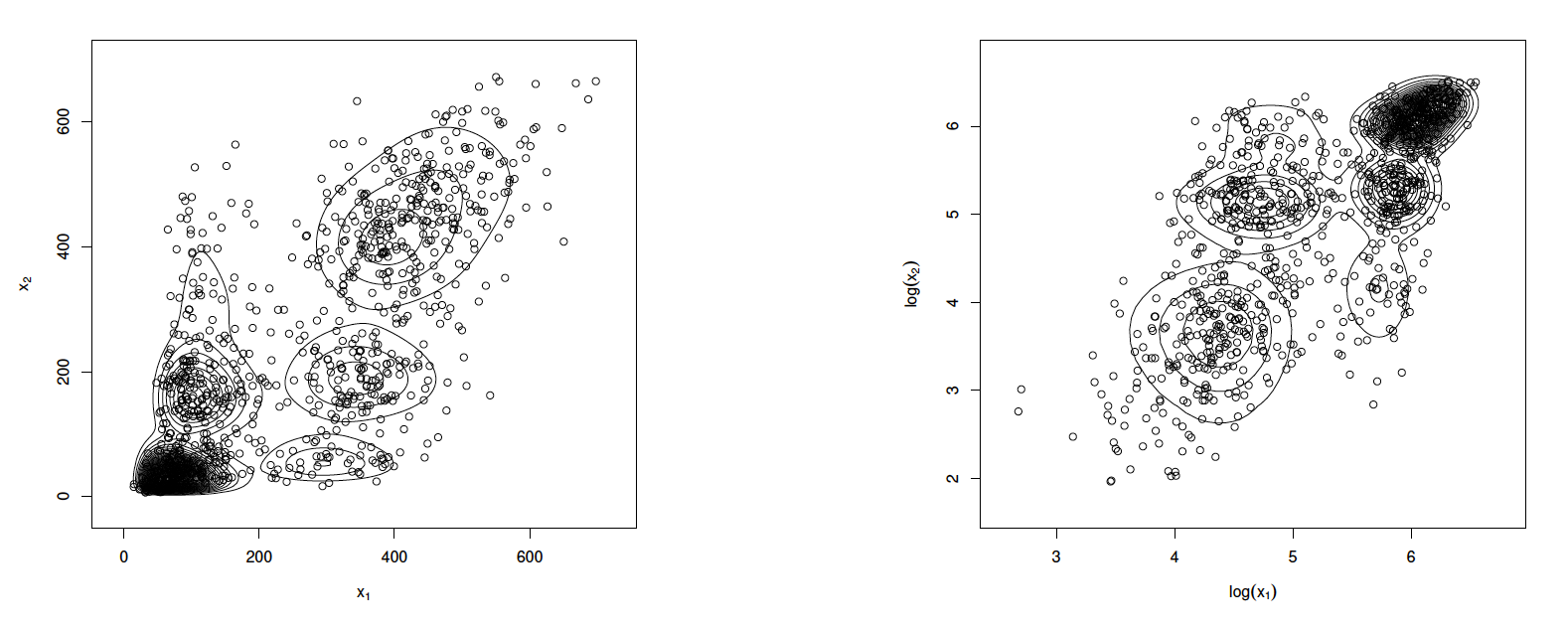
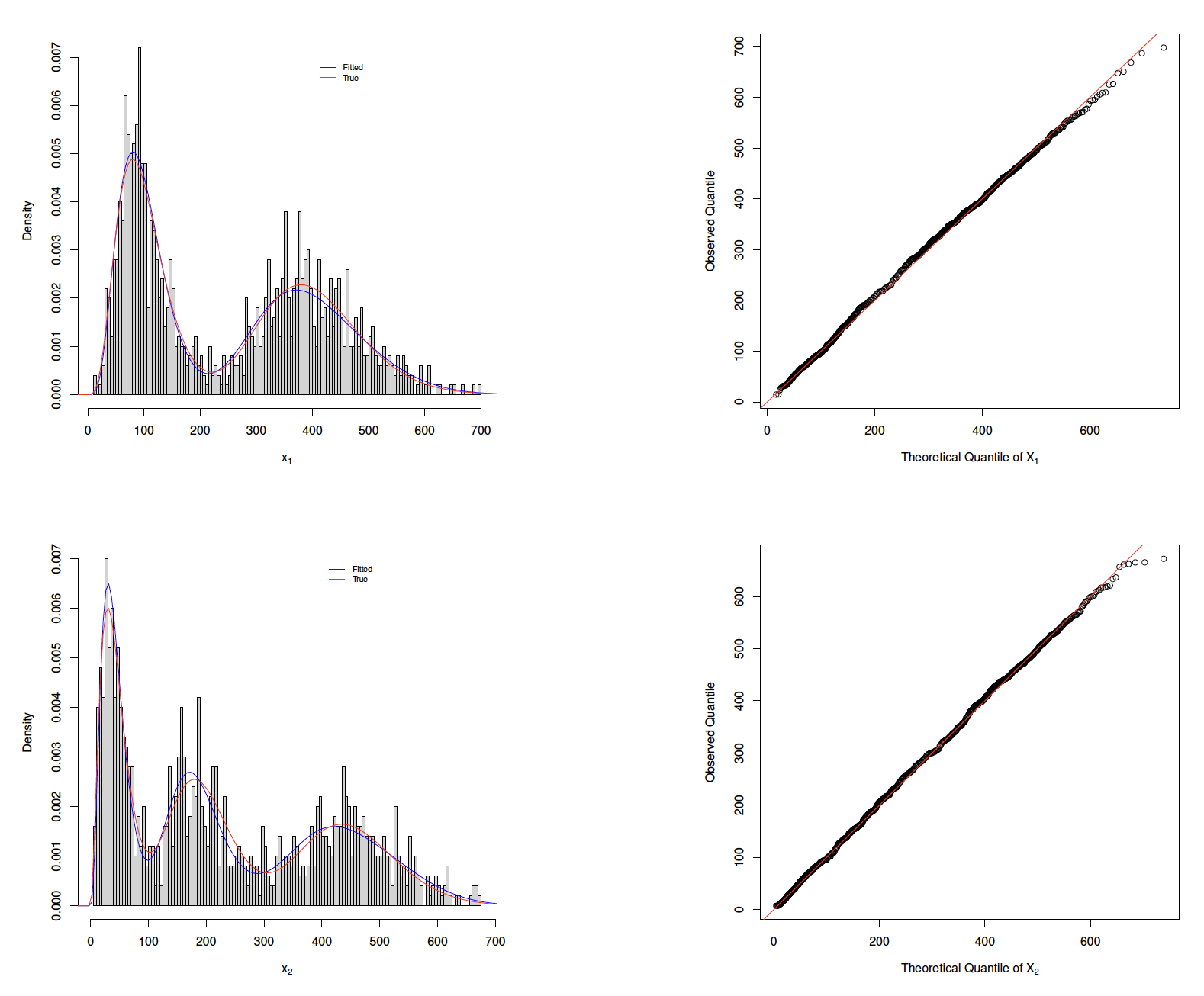
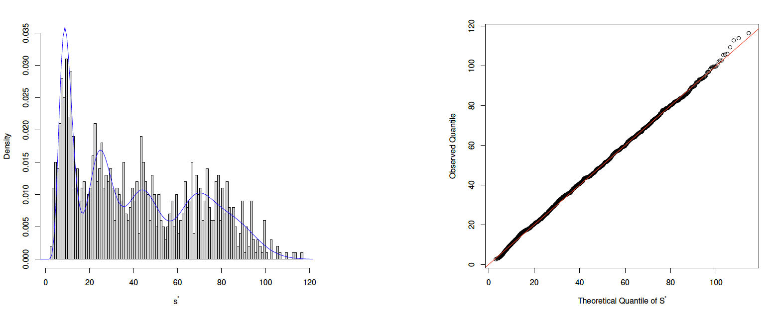
According to the AIC or BIC score, the Sheather and Jones method with $c = 1$ leads to the best fitting. The associated ${\rm MG}_2$ parameter estimates are summarized in Table 2. The marginal density estimates and the QQ plots of the fitted ${\rm MG}_2$ are shown in Figure 3. The contour plot of the bivariate density estimate is displayed in Figure 2. All of them imply that the proposed ${\rm MG}_2$ provides a good approximation of the data distribution. Another way to illustrate the bivariate goodness-of-fit is to assess the ${\rm MG}_2$ fitting against the standardized aggregate RV $S^* = {X_1}/{\hat{\theta}_1} + {X_2}/{\hat{\theta}_2}$ (S. C. K. Lee and Lin 2012; Verbelen et al. 2015). The study of the standardized aggregate RV effectively translates the bivarirate goodness-of-fit problem into a univaraite goodness-of-fit problem. By Propositions 5, the standardized aggregate RV $S^*$ follows a univaraite gamma mixtures distribution with a unit scale parameter. Based on the fitted ${\rm MG}_2$, the PDF of $S^*$ can be computed via

$$f_{S^*}(s)=\sum_{j=1}^m \widehat{\alpha}_j \frac{s^{\widehat{\gamma}_j^*-1}}{\Gamma\left(\widehat{\gamma}_j^*\right)} e^{-s}, \quad s>0$$

where $\widehat{\alpha}_j$ is the estimated mixture weight and $\widehat{\gamma}_j^*=\widehat{\gamma}_{1j}+\widehat{\gamma}_{2j}$, $j=1,\ldots,m$. The fitted density of $S^*$ and the associated QQ plot depicted in Figure 4 indicate a good fit.

Figure 2.Contour plots of the fitted density imposed over the original data (left-hand panel) and the logarithm transformed data (right-hand panel).

Figure 3.Histograms and QQ plots for the marginal distributions of $X_1$ and $X_2$.

Figure 4.Histogram and QQ plot for the standardized aggregation $S^*$ with the fitted density imposed over the left-hand panel.

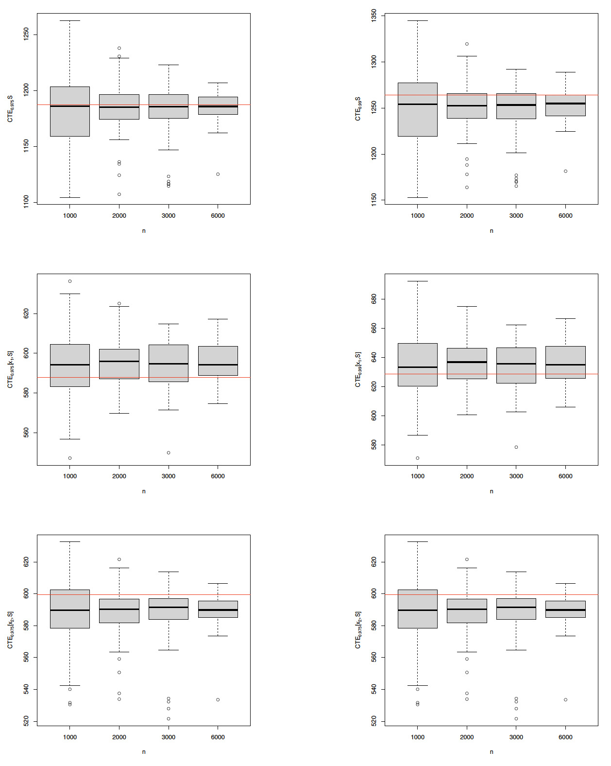
The fitted ${\rm MG}_2$ distribution can be adopted readily to estimate the CTE risk measure and allocation discussed in Section 2.1. In what follows, the simulation experiment is repeated $100$ times for each fixed sample size $n\in \{1,000,\ 2,000,\ 3,000,\ 6,000\}$. In each simulation trial, the ${\rm MG}_2$ distribution is fitted to the simulation data, based on which ${\mathrm{CTE}}_q[S_{\boldsymbol{X}}]$ and ${\mathrm{CTE}}_q[X_i;\,S]$ for $i=1,2$, and $q\in \{0.975,\ 0.99\}$ are computed according to Propositions 7 and 9. The box plots of the CTE estimates are displayed in Figure 5. For each box plot, the middle line is the median of the sampling distribution of the ${\rm MG}_2$ estimates; the lower and the upper limits of the box are the first and the third quartile, respectively; the upper (resp. lower) whisker extends up to 1.5 times the interquartile range from the top (resp. bottom) of the box; and the points are the outliers beyond the whiskers. For comparison purposes, the true values of related quantities are represented by the red reference lines in Figure 5, which are evaluated by $10^5$ times of simulations based on the true data-generating process specified at the beginning of this subsection. It is observed that as the sample size increases, the estimation interval shrinks. Moreover, all the estimate intervals cover the true CTE values, with the medians of the estimates’ being quite close to the true values.

Figure 5.Boxplots for the estimates of $\mathrm{CTE}_q\left[S_{\boldsymbol{X}}\right]$ and $\operatorname{CTE}_q\left[X_i ; S\right]$ for $i = 1, 2$, and $q \in\{0.975,0.99\}$, with the true values are specified by the red reference lines.

We also compare the performance of the proposed SGD-based ${\rm MG}_d$ fitting with the EM-based Erlang mixtures fitting considered in (Verbelen et al. 2015). Note that the implementation of the EM-based Erlang mixtures is very different from and much more involved than that of the proposed SGD-based ${\rm MG}_d$ fitting. For instance, the estimation procedure proposed in (Verbelen et al. 2015) requires the user to input the maximal number of mixture components allowed in each margin and keep dropping mixture components with small weights during the estimation process. Generally, the larger the number of mixture components initialized, the better the final fitting becomes, but the computation time is the trade-off. Moreover, the Erlang mixtures model relies on a common scale parameter shared by all the marginal distributions. Thus, the EM-based Erlang mixtures fitting is very sensitive to a fine-tuned scale parameter in the initialization step. For a fair comparison between the two methods, in the implementation of the EM-based Erlang mixtures fitting, we keep increasing the maximal number of mixture components used in the initialization step until the statistics fittings (e.g., likelihood value or AIC/BIC) of the two methods are about the same; then, based on that particular set of initialization inputs, the computation time is compared. The speeds reported were based on a desktop computer with the $64$-bit Windows $10$ operational system and a $3.4$ GHz CPU with $4$ physical cores.

We find that the computation speeds of the two methods are comparable in this simulation data set (see Table 3). The reasons are probably that the data-generating process itself has mixed Erlang marginal distributions and the scales of $X_1$ and $X_2$ are similar. Although the Erlang mixtures model contains only a common scale parameter, it is sufficient to handle this simulation data set. Because the underlying data-generating process is rather simple, the number of mixtures components needed is small, and the implementation of the EM algorithm is less complicated. However, as we will see in the subsequent examples, the proposed SGD-based ${\rm MG}_d$ fitting can significantly outperform the EM-based Erlang mixtures fitting when dealing with real-life data or simulation data with complicated data-generating processes.

4.2. Allocated loss adjustment expenses (ALAE) data

ALAE data studied in (Frees and Valdez 1998) are widely used as a benchmark data set for illustrating the usefulness of multivariate models. The data set contains $1,500$ general liability claims provided by Insurance Service Office, Inc. In each claim record, there is an indemnity payment denoted by $X_1$ and an ALAE denoted by $X_2$. Intuitively, the larger the loss amount is, the higher the ALAE becomes, so there is a positive dependence between $X_1$ and $X_2$. We approximate the joint distribution of $(X_1,X_2)$ by the ${\rm MG}_2$ distribution. The bandwidth-adjusting coefficient is tuned using the AIC score, and we conclude that Silverman’s method (Silverman 1986) with $c=1.5$ leads to the most desirable fitting. The histograms and density estimates of $X_1$, $X_2$, and $S^* = {X_1}/{\hat{\theta}_1} + {X_2}/{\hat{\theta}_2}$ using the ${\rm MG}_2$ distribution are displayed in Figure 6.

Figure 6.Histograms for $X_1$, $X_2$, and $S^*$ (left-hand panels) and the corresponding log transforms (right-hand panels) with the fitted MG₂ densities.

Based on the fitted ${\rm MG}_2$ distribution, Figure 7 presents the tail conditional expectation ${\mathrm{CTE}}_q[S_{\boldsymbol{X}}]$ and tail allocations ${\mathrm{CTE}}_q[X_1,S_{\boldsymbol{X}}]$ and ${\mathrm{CTE}}_{q}[X_2,S_{\boldsymbol{X}}]$ with varying $q\in (0,1)$. We observe that both ${\mathrm{CTE}}_q[X_1,S_{\boldsymbol{X}}]$ and ${\mathrm{CTE}}_{q}[X_2,S_{\boldsymbol{X}}]$ are increasing in $q$, which confirms the positive dependence relationship between $X_1$ and $X_2$. However, as $q$ increases, ${\mathrm{CTE}}_q[X_1,S_{\boldsymbol{X}}]$ increases at a faster rate than ${\mathrm{CTE}}_q[X_2,S_{\boldsymbol{X}}]$ does, and the distance between ${\mathrm{CTE}}_q[X_1,S_{\boldsymbol{X}}]$ and ${\mathrm{CTE}}_q[S_{\boldsymbol{X}}]$ gets narrower and narrower. In other words, compared with the ALAE, the indemnity payment amount is a more significant driver of large total payments.

Figure 7.The conditional tail expectations $\operatorname{CTE}_q\left[S_{\boldsymbol{X}}\right]$, $\operatorname{CTE}_q\left[X_1, S_{\boldsymbol{X}}\right]$, and $\operatorname{CTE}_q\left[X_2, S_{\boldsymbol{X}}\right]$, marked by the solid line, dashed line with circles, and dashed line with triangles, respectively.

Compared with the simulated mixed gamma data considered in Section 4.1, more mixture components in the ${\rm MG}_2$ distribution are needed in order to capture the highly right-skewed feature of the ALAE data. Specifically, $41$ mixture components are used to construct the density estimates presented in Figure 6. One can debate that the tail probability of the ${\rm MG}_d$ distribution decays exponentially, which may lead to underestimating the occurrence of extreme losses if the true data distribution—though it is never known in any real-life practice—followed a power law in the tail. To address the aforementioned concern, we can further impose a scale mixture structure on the multivariate mixed gamma or phase-type distributions (Bladt and Rojas-Nandayapa 2018; Furman, Kye, and Su 2021; Rojas-Nandayapa and Xie 2017), which are heavy tailed and still satisfy the universal approximation property. The application of the SGD method for fitting the multivariate scale mixtures of mixed gamma or phase-type distributions to heavy-tailed data is under active development in our ongoing research.

We again compare the performance of the SGD-based ${\rm MG}_d$ fitting with the EM-based Erlang mixtures fitting (Verbelen et al. 2015) on the ALAE data. Similar to the study in the previous example, we tune the maximal number of mixture components allowed in the initialization step of the EM-based Erlang mixtures fitting until the statistics fittings (e.g., likelihood value or AIC/BIC) of the two methods are comparable, and then based on the tuned initialization, the computation time is reported (see Table 4). As shown, the proposed SGD-based ${\rm MG}_d$ fitting method provides an appreciable improvement over the EM-based Erlang mixtures fitting method in that with even more final parameters to estimate, the SGD algorithm takes less than one third of the computation time of the EM algorithm. We believe that the improvement is attributed to the inclusion of heterogeneous scale parameters across different margins in the proposed ${\rm MG}_d$ model so the estimation is more robust to the scale parameters initialization as well as the computational elegance of SGD methods. This significant improvement of computational efficiency makes the SGD-based ${\rm MG}_d$ fitting more suitable for large-scale complex actuarial data analysis.

4.3. Capital allocation for a mortality risk portfolio

The last example demonstrates the application of the ${\rm MG}_d$ distribution to evaluating the capital allocation for a synthetic mortality risk portfolio motivated by (Van Gulick, De Waegenaere, and Norde 2012). The portfolio consists of three life insurance BLs.

• BL 1: A deferred single life annuity product that pays the insured a benefit of $1 per year if the insured is alive after age 65. Suppose that there are $n_1=45,000$ male insureds in BL 1. Let $t_{1j}$ and $\tau_{1j}$ denote, respectively, the present age and remaining lifetime of the $j$-th insured, $j=1,\ldots,n_1$ in this BL. Assuming that the maximal lifespan is $110$, the present value of total benefit payment in this BL can be computed via

$$X_1=\sum_{j=1}^{n_1} \sum_{k=\max \left(65-t_{1 j}\right)}^{110-t_{1 j}} \frac{\mathbf{1}\left(\tau_{1 j} \geq k\right)}{(1+r)^k}$$

where $r>0$ denotes the risk-free interest rate.

• BL 2: A survivor annuity product that pays the spouse of the insured a benefit of $0.75 per year if the insured dies before age 65. Suppose that there are $n_2=15, 000$ male insureds in BL 2. Let $t_{2j}$ and $\tau_{2j}$ denote, respectively, the present age and remaining lifetime of the $j$-th insured, $j=1,\ldots,n_2$, and similarly, $t_{2j}'$ and $\tau_{2j}'$ denote the present age and remaining lifetime of the spouse, respectively. The present value of total benefit payments in this BL can be computed via

$$\small{ X_2=0.75 \sum_{j=1}^{n_2} \sum_{k=0}^{110-t_{2 j}^{\prime}} \frac{\mathbf{1}\left(\tau_{2 j} \leq \min \left(k, 65-t_{2 j}\right)\right) \times \mathbf{1}\left(\tau_{2 j}^{\prime} \geq k\right)}{(1+r)^k} }$$

• BL 3: A life insurance product that pays a death benefit of $7.50 at the end of the death year if the insured dies before age 65. Suppose that there are $n_3=15, 000$ male insureds in BL 3. Let $t_{3j}$ and $\tau_{3j}$ denote, respectively, the present age and remaining lifetime of the $j$-th insured in this BL, $j=1,\ldots,n_3$. The present value of the total benefit payment in this BL can be computed via

$${X}_{3}=7.5 \sum_{j=1}^{n_3} \sum_{k=1}^{\max \left(65-t_{3 j}\right)} \frac{\mathbf{1}\left(k-1 \leq \tau_{3 j}<{k}\right)}{(1+r)^{k}}$$

In our study, we assume the risk-free interest rate to be $3\%$. We simulate the current ages of policyholders in the portfolio based on a discretized gamma distribution, and they will remain unchanged throughout the study. The distribution of the policyholders’ current ages is displayed in Figure 8.

Figure 8.The histogram of policyholders’ ages among BL’s 1 to 3.

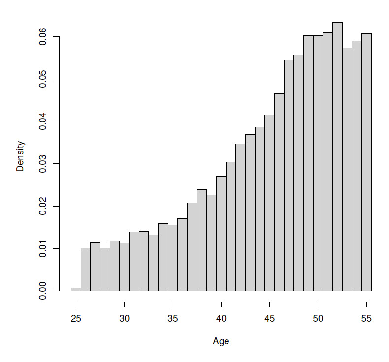
The liabilities of BLs 1 and 3 are driven by the longevity risk and mortality risk, respectively, while the interplay of these two risks determines the liability of BL 2. Using the StMoMo package (Millossovich, Villegas, and Kaishev 2018), we calibrate the classical (R. D. Lee and Carter 1992) mortality model based on the 1970–2016 U.S. mortality data extracted from the Human Mortality Database.^[2] The estimated mortality model is then used to generate $1,000$ mortality scenarios. Within the $j$-th mortality scenario, $j=1,\ldots,1,000$, the remaining lifetimes are simulated for every policyholder, and an observation of the present values of total payments $(x_{1j},x_{2j},x_{3j})$ is obtained. In the study of BL 2, we assume the remaining lifetimes of partners in a couple to be independent for simplicity. Our goal in this example is to evaluate the CTE-based capital allocations among the three BLs with the aid of the ${\rm MG}_3$ distribution.

Figure 9 presents the histograms of the simulated total benefit payments of the three BLs and the corresponding ${\rm MG}_3$ density estimates. The CTE-based capital allocations according to the fitted ${\rm MG}_3$ distribution are summaried in Table 5. As shown, the required aggregate risk capital increases as confidence level $q$ gets larger; so do the allocated capital amounts. Among the three BLs, most of the aggregate capital is apportioned to BL 1, which accounts for the largest portion of benefits paid out from the portfolio. As confidence level $q$ increases, the allocation percentage increases for BL 1 yet decreases for BL2 and BL 3. This implies that BL 1 becomes a more significant risk driver in the portfolio when the focus is shifted toward the tail region of the portfolio loss distribution. Recall that the liability of BL 1 is associated with longevity risk. The capital allocation results show that longevity risk plays a more decisive role than mortality risk in the insurance portfolio of interest.

Figure 9.The histograms of liability RV’s $X_1$, $X_2$, $X_3$, and the associated standardized sum $S^*=X_1 / \widehat{\theta_1}+X_2 / \widehat{\theta_2}+X_3 / \widehat{\theta_3}$

Finally, Table 6 summarizes the comparison of the SGD-based ${\rm MG}_d$ fitting with the EM-based Erlang mixtures fitting (Verbelen et al. 2015) based on the mortality risk data considered in this subsection. Recall that the maximal number of mixture components in the EM-based Erlang mixtures fitting is tuned such that the statistics fittings of the two methods are similar. As shown, the computation time required by the SGD-based ${\rm MG}_d$ fitting is more than 20 times faster than the EM-based Erlang mixtures fitting.

5. Conclusions

In this paper, we considered a class of multivariate mixtures of gamma distributions for modeling dependent insurance data. Distributional properties including marginal distributions, aggregate distribution, conditional expectations, and joint expectations were studied thoroughly. An estimation algorithm based on SGD methods was presented for the model estimation. Our numerical examples illustrated the practical usefulness of the ${\rm MG}_d$ distribution and the proposed estimation method.

We recognize a handful of topics for follow-up research. For instance, we are interested in exploring how various extensions of SGD methods can improve the efficiency of the estimation procedure for the ${\rm MG}_d$ distribution. Extending the SGD methods for fitting the ${\rm MG}_d$ distribution to censored and/or truncated data should be addressed in future research. Another future research topic is related to the scale mixtures of ${\rm MG}_d$ distributions for handling heavy-tailed data.

Acknowledgments

We are indebted to two anonymous referees for their very thorough reading of the paper and thank them for the many suggestions that resulted in an improved version. We are grateful to the Casualty Actuarial Society for its generous financial support of our research.