Statistical Models and Algorithms for Assessing Robustness and Reliability of Networks with Applications in Cybersecurity Insurance

1. Introduction

Many complex networks, such as cyberspace, the Internet, power grids, are critical infrastructures for commerce and communications that require extremely high reliability and safety standard. Significant attacks or failures on those complex networks could cause serious damage to society. Insurance is one of the possible ways to manage risk exposure for these complex networks. For example, cybersecurity insurance is designed to mitigate losses from a variety of cyber incidents, including data breaches, business interruption, and network damage (Department of Homeland Security 2019). In 2013, the Group of Twenty (G-20) urged to treat cyber-attacks as a threat to the global economy (Ackerman 2013). For the data and statistics from government, industry, and information technology related to the current state of cybersecurity threats in the United States and internationally, one can refer to (Tehan 2015). Recently, (Böhme, Laube, and Riek 2019) provided a general framework for actuaries to think about cyber risk and the approaches to cyber risk analysis. In this paper, “cyberspace” refers to the interactive domain composed of all digital networks used to store, modify, and communicate information, and the term “cyber risk” refers to a multitude of different sources of risk affecting the information and technology assets of a company (Biener, Eling, and Wirfs 2014). Since the internet is one of the most complex systems humanity has ever devised, cyber risk management becomes a prominent issue for society, especially for insurance companies (Zurich Insurance Company Ltd and Atlantic Council of the United States 2014). However, research on cyber risk, especially on evaluation and comparison of the risks in the insurance domain, is fairly limited. In addition, pricing for cybersecutiry insurance is a challenging problem since sybersecutiry insurance has no standard scoring systems or actuarial tables for rate making (Xu and Hua 2017). Moreover, there is a lack of open-source data for organizations’ internal networks for security breaches and losses due to the disinclination of organizations to disclose details of security breaches. As Böhme, Laube, and Riek (2019) pointed out, understanding cyber risk is a hard problem, therefore, comprehending how vulnerable is a cyber or physical network to attacks or failures and assessing the risks of a complex network is of great interest. There is an urgent need to develop advanced methodologies that can systematically assess the risk, robustness, reliability, or loss of availability of a network and comparing the risk and robustness of different networks.

Cyber risk is a fundamental measurement providing a quantitative measure of the security level, the capability of capturing attacks, and the lost of availability that results in loss of integrity and availability (Biener, Eling, and Wirfs 2014; Böhme, Laube, and Riek 2019). To evaluate the loss of availability of cyber networks, various heuristic methods were proposed to measure the resilience of cyber networks under malicious cyber attacks (Vespignani 2010; Havlin et al. 2014). However, those heuristic methods are often designed for a specific cyber network, which limited their applicability to diverse areas (Kotenko, Saenko, and Lauta 2018). In general, metric-based approaches use specific measures of individual properties of cyber system components to access resilience. For example, when evaluating the resilience of a computer system, (Ganin et al. 2016) considered the percentage of computers that are functioning and the ratio of a system’s actual flow to its maximum capacity for measuring resilience. This metric-based approach may not be appropriate for systems that the connections between the nodes (computers) have an important effect on the resilience of the system. Therefore, some high-order structures and topological measures of a network should be considered.

In managing cyber risk in the insurance domain, different tools and methods have been proposed for evaluating the network robustness in the past decades, however, algorithms/techniques based on statistical models and stochastic processes have not been broadly developed. In this paper, we aim to develop dependable and flexible statistical models and hypothesis testing procedures to assess the risk and robustness of a complex network which can provide useful information for cyber insurance providers. Specifically, we propose a modified Wiener process model with several statistical hypothesis testing procedures for this purpose. The Wiener process model is one of the widely used stochastic models for non-monotonic degradation processes which can provide a good description of the system’s behavior in the cascading failure process (Doksum, Hóyland, and Hoyland 1992; Chen et al. 2017; Lio et al. 2019). Compared with observing dynamics of the topological measures under attacks, the proposed modified Wiener process model can model the evolution of the degradation data in each network topological measure and also provide great flexibility in degradation modeling, e.g., non-linear degradation mechanisms. The proposed methodologies will expand the actuarial knowledge on the evaluation and comparison of risks for different physical and/or cyber networks and cybersecurity insurance pricing models.

The rest of this paper is organized as follows. In Section 2, the graph representation of the cyber network and the topological measures for evaluating the robustness/loss of availability of a network are discussed. In Section 3, the proposed Wiener process model for modeling the dynamics of a cyber network losing its functionality/connectivity upon the removal of nodes is presented. The proposed statistical testing procedures for comparing the risks of two networks are also presented in Section 3. In Section 4, illustrative examples based on real data sets of the Gnutella peer-to-peer (P2P) cyber networks and sampled subgraphs from the Enron email network are given in Section 4. A Monte Carlo simulation study is used to evaluate the performance of the proposed model and methods in Section 5. The performance and limitations of the proposed methods are discussed. Finally, in Section 6, some concluding remarks are provided.

2. Graph Representation of Cyber Network

Inherently, a cyber network, such as the P2P cyber network, can be viewed as a graph structure consisting of nodes and edges. For example, in a P2P cyber network, the hosts are considered as nodes in a graph, and the host’s neighbor set is described by the set of edges in a graph. A graph structure can be represented as $\mathcal{G} = \{\mathcal{V}, \mathcal{E}, W$}, where $\mathcal{V}$ is a node set with cardinality (the number of elements in a set) $|\mathcal{V}|$ of $N$, $\mathcal{E} \subseteq \mathcal{V} \times \mathcal{V}$ is an edge set, and $W$ is the adjacency matrix of $\mathcal{G}$, which is an $N \times N$ nonnegative symmetric matrix with entries $\{\omega_{ij}\}_{1\leq i,j\leq N}$, i.e., $\omega_{ij} \neq 0$ for any $e_{i j} \in \mathcal{E}$ and $\omega_{ij} = 0$, otherwise. In the study of cyber network, we consider unweighted and undirected graph, i.e., $\omega_{ij} = 1$ and $e_{ij} = e_{ji} \in \mathcal{E}$, for all $1 \leq i, j \leq N$. Hence, we suppress the notation of the adjacency matrix in the graph representation and represent the graph as $\mathcal{G} = \{\mathcal{V}, \mathcal{E}\}$.

To evaluate the robustness/loss of availability of a network, the decrease of network performance due to a selected removal of nodes or edges is considered. For example, in cyberspace, computers and hand-held devices are connected to servers over active Internet signals or local area network (LAN) lines. In this case, those computers, hand-held devices, and servers are the nodes and the LAN lines and Internet signals are edges of the network graph of interest. The failure of a server or broken LAN lines (due to physical or cyber attacks, or human errors) will reduce the functionality of the cyber network.

High-order structures are often called the building blocks of network (Maison et al. 2002). Compared with global network topology (e.g., graph diameter and average path length) (Cohen et al. 2000; Piraveenan, Uddin, and Chung 2012; Cuadra et al. 2015), through studying the high-order structures, we can capture more local information of network structure. For instance, feedforward loops have proven fundamental to understanding the mechanism of transcriptional regulation networks (Shen-Orr et al. 2002). Here, the robustness of a cyber network can be defined as the ability of a network to maintain its functionality/connectivity when it is subject to failure or attack. There is a variety of graph measures that provide robustness measures on a network (Newman 2010). For example, vertex connectivity is defined as the minimum number of vertices that need to be removed to disconnect the graph and the average cluster coefficient that represents the probability that neighbors of a node are also connected (Holland and Leinhardt 1971; Watts and Strogatz 1998). Another commonly used robustness measure is the network motifs introduced by (Milo et al. 2002) in conjunction with the assessment of the stability of biological networks and later have been studied in a variety of contexts (Alon 2007). Network motifs are subgraphs (smaller patterns) that the numbers of appearances are statistically significantly greater than a predefined threshold in a randomized network. A motif here is broadly defined as a recurrent multi-node subgraph pattern. Formally, a motif is an induced subgraph of $\mathcal{G}$. Figure 1 shows all possible 4-node motifs in undirected graph. Recently, Dey, Gel, and Poor (2019) focused on incorporating network motifs to evaluate and estimate the power system reliability with the help of statistical models.

Figure 1.All connected 4-node network motifs.

To obtain the exact motif counts of different motif types in a specific $k$-size motif in a network, the RANDESU motif finder algorithm (Holland and Leinhardt 1970) can be used. For large network (> 10,000 edges), algorithms to approximate the exact motif counts can be used (Kashtan et al. 2004; Böhme, Laube, and Riek 2019), which introduces another layer of randomness in the data whereas suitable statistical models and techniques are required. To assess the robustness of a complex network like the cyber network, we focus on remaining motif distributions under various attacks like the physical or cyber-attack and cascading failure of attacks.

3. Wiener Process Model and Similarity Tests for Networks

In this paper, we assume that either the exact or approximate measures of network robustness can be obtained and focus on the development of novel statistical algorithms to assess the robustness and the risk, as well as to compare the risks of different networks. Although the methods described here focuses on network motifs, the proposed methodologies can be applied to any topological measures of network robustness/risk such as the Wasserstein distance and the weighted-pairwise distance. The process of reducing the functionality of the physical or cyber networks under removal of nodes and/or edges can be viewed as a degradation process (Chen et al. 2017) and hence, novel statistical models and algorithms for degradation data analysis can be applied to evaluate and compare the risks of different complex networks.

In this section, we investigate how local topological features (e.g., local network structures) evolve under the removal of nodes and/or edges. Our main postulate here is that a complex system can be considered more resilient if it tends to preserve its original properties longer under the removal of nodes and/or edges, and our primary focus is to quantify the risks of different networks through statistical modeling and analyses of the geometric properties of different network systems. A stochastic model, the Wiener process model, along with several statistical hypothesis testing procedures to compare the risks of different networks are developed. The mathematical notation and the Wiener process model are introduced in Section 3.1 and three statistical hypothesis testing procedures are proposed in Section 3.2.

3.1. Wiener process model

Suppose that there are $\mathcal{I}$ networks and $\mathcal{J}$ different topological features (e.g., network motifs, Wasserstein distance, and weighted-pairwise distance, etc.) are used to measure the risks of those $\mathcal{I}$ networks, these topological features are observed at different time points $t_{k}$, $k=0, 1, \ldots, \mathcal{K}$, where $\mathcal{K} + 1$ is the total number of observation points. The observation point $t_k$ can be considered as a specific fraction of random/selective nodes (e.g., nodes with the highest degrees or nodes with the largest betweenness) being removed from the network. We denote the observed value of the $j$-th topological feature for network $i$ at the $k$-th time point as $y_{i,j,k}$. For example, consider the 4-node motif $M_{1}$ in Figure 1 as the $j$-th topological feature, then $y_{i,j,0}$ is the number of the 4-node motif $M_{1}$ in network $i$ when all the nodes and edges in the network are fully functioning (i.e., at time $t_{0}$), $y_{i,j,1}$ is the number of the 4-node motif $M_{1}$ in network $i$ when 10% of the nodes and edges in the network are removed (say, at time $t_{1}$), $y_{i,j,2}$ is the number of the 4-node motif $M_{1}$ in network $i$ when 20% of the nodes and edges in the network are removed (say, at time $t_{2}$), and so on.

Since the dynamics of the local topological measures upon removal of the nodes/edges may not necessarily be a monotonic deterioration process and due to the stochastic nature of this process, we thus propose using the Wiener process model to characterize the degradation paths of those topological measures of a complex network. We consider modeling the degeneration process of the functionality of the $i$-th network based on the $j$-th topological measure by using a Wiener process with drift parameter $\mu_{i,j}^*$ and diffusion coefficient $\sigma_{i,j}^*$. Specifically, we consider $D_{i,j}(t_k) = 1 - y_{i,j,k}/ y_{i,j,0}$ as a stochastic process $\{D_{i,j}(t_k), t_k \geq 0\}$, which is characterized by the following properties:

(i) $D_{i,j}(t_0) = 1 - y_{i,j,0}/y_{i,j,0} = 0$;

(ii) $\{D_{i,j}(t_k), t_k \geq 0\}$ has stable independent increments, i.e., the increments $D_{i,j}(t_k) - D_{i,j}(t_{k-1})$, $k = 1, 2, \ldots, \mathcal{K}$ are independent;

(iii) the increments $D_{i,j}(t_k) - D_{i,j}(t_{k-1})$ follows a normal distribution $\mathcal{N}(\mu^{*}_{i,j}, {\sigma_{i,j}^{*2}})$.

Since different topological measures may share similar characteristics, therefore, we modify the Wiener process model by introducing a correlation structure among the $\mathcal{J}$ topological measures. Based on the modified Wiener process model, in our study, we define a $\mathcal{J}$-dimensional vector of random variables $\pmb{x}_{i,k} = (x_{i,1,k}, x_{i,2,k}, \ldots, x_{i,\mathcal{J},k})^{\prime} \in \mathbb{R}^{\mathcal{J}}$, where $x_{i,j,k} = (y_{i,j,k} - y_{i,j,k+1})/y_{i,j,0}$, $i = 1, 2, \ldots, \mathcal{I}$; $j = 1, 2, \ldots, \mathcal{J}$; $k = 0, 1, 2, \ldots, \mathcal{K}$, and assume that the degradation process follows a Wiener process with drift $\pmb{\mu}_i$ and variance-covariance $\pmb{\Sigma}_i$. In other words, the $\mathcal{J}$-dimensional vector of random variables $\pmb{x}_{i,k} = (x_{i,1,k},x_{i,2,k},\dots, x_{i,\mathcal{J},k})^{\prime} \in \mathbb{R}^{\mathcal{J}}$ follows a $\mathcal{J}$-dimensional multivariate normal distribution denoted as

$$\mathcal{M}_W: \pmb{x}_{i,k} \sim \mathcal{N}_{\mathcal{J}}(\pmb{\mu}_i, \pmb{\Sigma}_i),\tag{1}$$

where $\pmb{\mu}_i = (\mu_{i1}, \dots, \mu_{i\mathcal{J}})^{\prime} \in \mathbb{R}^{\mathcal{J}}$ represents the slope of the linear drift and $\pmb{\Sigma}_i$ represents an $\mathcal{J} \times \mathcal{J}$ symmetric variance-covariance matrix

$$\pmb{\Sigma}_i = \begin{pmatrix} \sigma_{i,11} & \sigma_{i,12} & \cdots & \sigma_{i,1\mathcal{J}} \\ & \sigma_{i,22} & \cdots & \sigma_{i,2\mathcal{J}} \\ & & \ddots & \vdots \\ & & & \sigma_{i,\mathcal{J}\mathcal{J}} \end{pmatrix}\tag{2}$$

which is also known as the diffusion coefficient. The joint probability density function of the random vector $\pmb{x}_{i,k}$ is

$$\scriptsize{ f(\pmb{x}_{i,k};\pmb{\mu}_i, \pmb{\Sigma}_i) = \frac{1}{(2\pi)^{\mathcal{J}/2}|\pmb{\Sigma}_i|^{1/2}}\exp{\left\{\frac{(\pmb{x}_{i,k}-\pmb{\mu}_i)^{\prime}\pmb{\Sigma}_i^{-1}(\pmb{x}_{i,k}-\pmb{\mu}_i)}{2}\right\}},\tag{3} }$$

for $\pmb{x}_{i,k} \in \mathbb{R}^{\mathcal{J}}$. Under this setting, the log-likelihood function can be expressed

$$\ln L(\pmb{\theta}|\pmb{x}) = \sum_{i=1}^{\mathcal{I}}\ln L_{i}(\pmb{\theta}_i|\pmb{x}_i),\tag{4}$$

where $\pmb{x} = (\pmb{x}_1, \dots, \pmb{x}_\mathcal{I})$, $\pmb{\theta} = (\pmb{\theta}_1, \dots, \pmb{\theta}_{\mathcal{I}})$,

$$\scriptsize{ \begin{align} &\ln L\left(\pmb{\theta}_i \mid \pmb{x}_i\right)\\ &\quad =\sum_{k=1}^{\mathcal{K}}\left[-\frac{\mathcal{J}}{2} \ln (2 \pi)-\frac{1}{2} \ln \left(\left|\Sigma_i\right|\right)-\frac{1}{2}\left(\pmb{x}_{i, k}-\pmb{\mu}_i\right)^{\prime} \Sigma_i^{-1}\left(\pmb{x}_{i, k}-\pmb{\mu}_i\right)\right], \end{align} \tag{5} }$$

and $\pmb{\theta}_i$ = $\{(\pmb{\mu}_i, \pmb{\Sigma}_i)|\pmb{\mu}_i \in \mathbb{R}^{\mathcal{J}}, \pmb{\Sigma}_i$ is an $\mathcal{J}\times \mathcal{J}$ positive-semidefinite matrix is the parameter vector for the $i$-th network. The maximum likelihood estimates (MLEs) of the model parameters can be obtained by maximizing $\ln L(\pmb{\theta}_i|\pmb{x}_{i})$ in Eq. (5) with respect to $\pmb{\mu}_i$ and $\pmb{\Sigma}_i$. Iterative numerical algorithms for solving a non-linear system of equations with constraints, such as the limited-memory Broyden-Fletcher-Goldfarb-Shanno algorithm for box constraints (L-BFGS-B algorithm), can be utilized here to obtain the MLEs.

3.2. Similarity tests for two complex networks

In this subsection, we consider three different statistical procedures for testing the similarity of two complex networks (say, Network 1 and Network 2) in terms of their resilience/risk level based on the $\mathcal{J}$ topological measures. We are interested in testing the hypotheses

$$\small{\begin{aligned} H_0: \quad &\mbox{Network 1 and Network 2} \\ & \mbox{have the same resilience/risk level} \\ {\mbox {against }} H_{1}: \quad &\mbox {Network 1 and Network 2} \\ &\mbox{do not have the same resilience/risk level} \end{aligned} \tag{6}}$$

3.2.1. A test procedure based on resampling

The first proposed testing procedure is based on the Euclidean distance of degradation curves with resampling approach. Based on the observed degradation measurements $\vec{\pmb{x}}_{1} = \{\pmb{x}_{1,1}, \pmb{x}_{1,2}, \cdots, \pmb{x}_{1,\mathcal{K}}\}$ and $\vec{\pmb{x}}_{2}= \{\pmb{x}_{2,1}, \pmb{x}_{2,2}, \cdots, \pmb{x}_{2,\mathcal{K}} \}$ from Network 1 and Network 2, respectively, the algorithm to compute the $p$-value for testing the hypotheses in (6) is described here. We name this procedure as Procedure A.

Step A1: Compute the Euclidean distance between $\vec{\pmb{x}}_{1} = \{\pmb{x}_{1,1}, \pmb{x}_{1,2}, \cdots, \pmb{x}_{1,\mathcal{K}}\}$ and $\vec{\pmb{x}}_{2}= \{\pmb{x}_{2,1}, \pmb{x}_{2,2}, \cdots, \pmb{x}_{2,\mathcal{K}} \}$ for the two networks: $$d_{obs} = d_{obs}(\vec{\pmb{x}}_{1}, \vec{\pmb{x}}_{2}) = \left[\sum_{k=1}^{\mathcal{K}}\sum_{j=1}^{\mathcal{J}}(\pmb{x}_{1,k}- \pmb{x}_{2,k})^2\right]^{1/2}.$$

Step A2: Combine the two sets of observed degradation measurements and denote the combined data set as $\vec{\pmb{x}}_{C} = (\vec{\pmb{x}}_{1},\vec{\pmb{x}}_{2})$. Based on the Wiener process model in Eq. (1), obtain the MLE of $\pmb{\theta} = (\pmb{\mu}, \pmb{\Sigma})$ by maximizing the log-likelihood function $\ln L(\pmb{\theta}, \vec{\pmb{x}}_{C})$ in Eq. (5) with respect to $\pmb{\theta}$. The MLE of $\pmb{\theta}$ based on the combined data set under $H_{0}$ in (6) is denoted by ${\pmb{\hat \theta}}_{C} = ({\pmb{\hat \mu}}_{C}, {\pmb{\hat \Sigma}}_{C})$.

Step A3: Generate ${\pmb{x}}^{(1)}_{1,k}$ and ${\pmb{x}}^{(1)}_{2,k}$ from a ${\mathcal{J}}$-dimensional multivariate normal distribution $\mathcal{N}_{\mathcal{J}}({\pmb{\hat \mu}}_{C}, {\pmb{\hat \Sigma}}_{C})$, for $k = 1, 2, \ldots, \mathcal{K}$, to obtain the parametric bootstrap samples $\vec{\pmb{x}}^{(1)}_1 = \{{\pmb{x}}^{(1)}_{1,1}, {\pmb{x}}^{(1)}_{1,2}, \ldots, {\pmb{x}}^{(1)}_{1,\mathcal{K}}\}$ and $\vec{\pmb{x}}^{(1)}_2 = \{{\pmb{x}}^{(1)}_{2,1}, {\pmb{x}}^{(1)}_{2,2}, \ldots, {\pmb{x}}^{(1)}_{2,\mathcal{K}}\}$, respectively.

Step A4: Compute the Euclidean distance between the two parametric bootstrap samples $\vec{\pmb{x}}^{(1)}_1$ and $\vec{\pmb{x}}^{(1)}_2$ as $$d^{(1)} = d^{(1)}(\vec{\pmb{x}}^{(1)}_1, \vec{\pmb{x}}^{(1)}_2) = \left[\sum_{k=1}^{\mathcal{K}}\sum_{j=1}^{\mathcal{J}}(\pmb{x}^{(1)}_{1,k}- \pmb{x}^{(1)}_{2,k})^2\right]^{1/2}.$$

Step A5: Repeat Steps A3–A4 $B$ times to obtain a sequence of bootstrap Euclidean distances, $d^{(b)} = d^{(b)}(\vec{\pmb{x}}^{(b)}_1,\vec{\pmb{x}}^{(b)}_{2})$, for $b= 1, 2, \dots, B$.

Step A6: The $p$-value of the test is computed as $$p_{A} = \frac{1}{B} \sum\limits_{b = 1}^{B} 1_{\{d_{obs}>d^{(b)}\}},$$ where $1_{\{A\}}$ is an indicator function defined as $1_{\{A\}} = 1$ if event $A$ is true and $1_{\{A\}} = 0$ otherwise.

The null hypothesis in (6) is rejected if $p_{A} < \alpha$, where $\alpha$ is a prefixed significant level. Note that Procedure A only uses the Wiener process model in the resampling process in Steps A3 and A4. In this procedure, we use the Euclidean distance as a measure of the distance between two vectors, however, other types of distance metrics such as the Manhattan distance can be used in place of the Euclidean distance.

3.2.2. Test procedures based on likelihood ratio test statistic

Under the Wiener process model described in Section 3.1, the hypotheses in (6) can be expressed as

$$\begin{aligned} H_0: \quad & \pmb{\mu}_1=\pmb{\mu}_2=\pmb{\mu} \text { and } \pmb{\Sigma}_1=\pmb{\Sigma}_2=\pmb{\Sigma} \\ \text { against } H_1: \quad & \pmb{\mu}_1 \neq \pmb{\mu}_2 \text { or } \pmb{\Sigma}_1 \neq \pmb{\Sigma}_2 . \end{aligned} \tag{7}$$

Let $\pmb{\hat \theta}_i = (\pmb{\hat \mu}_i, \pmb{\hat \Sigma}_i)$ be the MLE of the $\pmb{\theta}_i$ that maximizes the log-likelihood function $\ln L(\pmb{\theta}_{i}, \vec{\pmb{x}}_{i})$ in Eq. (5) with respect to $\pmb{\theta}_{i}$ based on the data $\vec{\pmb{x}}_{i}$, i.e.,

$$\begin{aligned} \pmb{\hat \theta}_i = \mathop{\mathrm{arg\,max}}_{\pmb\theta_i} \ln L(\pmb{\theta}_{i}, \vec{\pmb{x}}_{i}), \end{aligned}\tag{8}$$

for $i = 1, 2$. Similarly, based on the combined data set $\vec{\pmb{x}}_{C} = (\vec{\pmb{x}}_{1},\vec{\pmb{x}}_{2})$, the MLE of $\pmb{\theta_{C}} = (\pmb{\mu}_C, \pmb{\Sigma}_C)$ that maximizes the log-likelihood function $\ln L(\pmb{\theta}_C, \vec{\pmb{x}}_{C})$ in Eq. (5) with respect to $\pmb{\theta}_C$ under $H_{0}$ in (7) is denoted as $\pmb{\hat \theta}_C$, i.e.,

$$\hat{\boldsymbol{\theta}}_C=\underset{\boldsymbol{\theta}_C}{\arg \max } \ln L\left(\boldsymbol{\theta}_C, \overrightarrow{\boldsymbol{x}}_C\right) . \tag{9}$$

The likelihood ratio test statistic based on $\vec{\pmb{x}}_{1}$ and $\vec{\pmb{x}}_{2}$ is defined as

$$\Lambda\left(\overrightarrow{\pmb{x}}_1, \overrightarrow{\pmb{x}}_2\right)=-2 \ln \left[\frac{L\left(\hat{\pmb{\theta}}_C, \overrightarrow{\pmb{x}}_C\right)}{L\left(\hat{\pmb{\theta}}_1, \overrightarrow{\pmb{x}}_1\right) \times L\left(\hat{\pmb{\theta}}_2, \overrightarrow{\pmb{x}}_2\right)}\right] . \tag{10}$$

The Neyman–Pearson lemma states that the likelihood ratio test is the most powerful test at significance level $\alpha$. As the sample size approaches $\infty$, the test statistic $\Lambda(\vec{\pmb{x}}_{1}, \vec{\pmb{x}}_{2})$ is asymptotically chi-squared distribution with degrees of freedom $q = \mathcal{J} + \mathcal{J}(\mathcal{J}+1)/2$. Two statistical hypothesis test procedures, namely Procedure B1 and Procedure B2, are developed here based on the likelihood ratio test statistic in Eq. (10). The $p$-value of Procedure B1 is obtained based on the asymptotic distribution of the likelihood ratio test statistic $\Lambda(\vec{\pmb{x}}_{1},\vec{\pmb{x}}_{2})$, while the $p$-value of Procedure B2 is obtained based on resampling technique.

Based on the observed degradation measurements $\vec{\pmb{x}}_{1} = \{\pmb{x}_{1,1}, \pmb{x}_{1,2}, \cdots, \pmb{x}_{1,\mathcal{K}}\}$ and $\vec{\pmb{x}}_{2}= \{\pmb{x}_{2,1}, \pmb{x}_{2,2}, \cdots, \pmb{x}_{2,\mathcal{K}} \}$ from Network 1 and Network 2, respectively, the algorithm to computer the $p$-value for Procedures B1 and B2 can be described as follows:

Step B1: Obtain the MLE of $\pmb{\theta}_{i} = (\pmb{\mu}_{i}, \pmb{\Sigma}_{i})$ from $\vec{\pmb{x}}_{i}$, $i = 1,2$ based on Eq. (8).

Step B2: Combine the two sets of observed degradation measurements $\vec{\pmb{x}}_{C} = (\vec{\pmb{x}}_{1},\vec{\pmb{x}}_{2})$ and obtain the MLE of $\pmb{\theta}_{C} = (\pmb{\mu}_{C}, \pmb{\Sigma}_{C})$ from $\vec{\pmb{x}}_{C}$ based on Eq. (9).

Step B3: Compute the likelihood ratio test statistic $\Lambda_{obs} = \Lambda(\vec{\pmb{x}}_{1}, \vec{\pmb{x}}_{2})$ from Eq. (10).

Step B4: For Procedure B1, the $p$-value is computed as

$$p_{B1} = \Pr(W \lt \Lambda_{obs})$$

where $W$ is random variable that follows a chi-square distribution with degrees of freedom $q = \mathcal{J} + \mathcal{J}(\mathcal{J}+1)/2$.

Step B5: Generate ${\pmb{x}}^{(1)}_{1,k}$ and ${\pmb{x}}^{(1)}_{2,k}$ from a ${\mathcal{J}}$-dimensional multivariate normal distribution $\mathcal{N}_{\mathcal{J}}({\pmb{\hat \mu}}_{C}, {\pmb{\hat \Sigma}}_{C})$, for $k = 1, 2, \ldots, \mathcal{K}$, to obtain the parametric bootstrap samples $\vec{\pmb{x}}^{(1)}_1 = \{{\pmb{x}}^{(1)}_{1,1}, {\pmb{x}}^{(1)}_{1,2}, \ldots, {\pmb{x}}^{(1)}_{1,\mathcal{K}}\}$ and $\vec{\pmb{x}}^{(1)}_2 = \{{\pmb{x}}^{(1)}_{2,1}, {\pmb{x}}^{(1)}_{2,2}, \ldots, {\pmb{x}}^{(1)}_{2,\mathcal{K}}\}$, respectively.

Step B6: Compute the likelihood ratio test statistic based on the two parametric bootstrap samples as $\Lambda^{(1)} = \Lambda(\vec{\pmb{x}}^{(1)}_{1}, \vec{\pmb{x}}^{(1)}_{2})$ from Eq. (10).

Step B7: Repeat Steps B4’–B5’ $B$ times to obtain a sequence of bootstrap likelihood ratio test statistics, $\Lambda^{(b)} = \Lambda(\vec{\pmb{x}}^{(b)}_{1}, \vec{\pmb{x}}^{(b)}_{2})$, for $b= 1, 2, \dots, B$.

Step B8: For Procedure B2, the $p$-value is computed as

$$p_{B2} = \frac{1}{B} \sum\limits_{b = 1}^{B} 1_{\{\Lambda_{obs} < \Lambda^{(b)}\}}.$$

The null hypothesis in (7) is rejected if $p_{B1} < \alpha$ for Procedure B1, and if $p_{B2} < \alpha$ for Procedure B2, where $\alpha$ is a prefixed significant level.

4. Practical Data Analysis

In this section, we illustrate the proposed model and methods by analyzing two real network data sets for P2P service and email systems, which are two kinds of cyber systems that requires cybersecurity insurance. The background of the network data sets is presented in Section 4.1.1 and Section 4.2.1, and the results and discussions of the data analysis are presented in Section 4.1.2 and Section 4.2.2.

We also provide an illustration of actuarial applications of the proposed methodologies based on the P2P networks in Section 4.1.3.

4.1. Peer-to-peer network

4.1.1. Background of the peer-to-peer network datasets

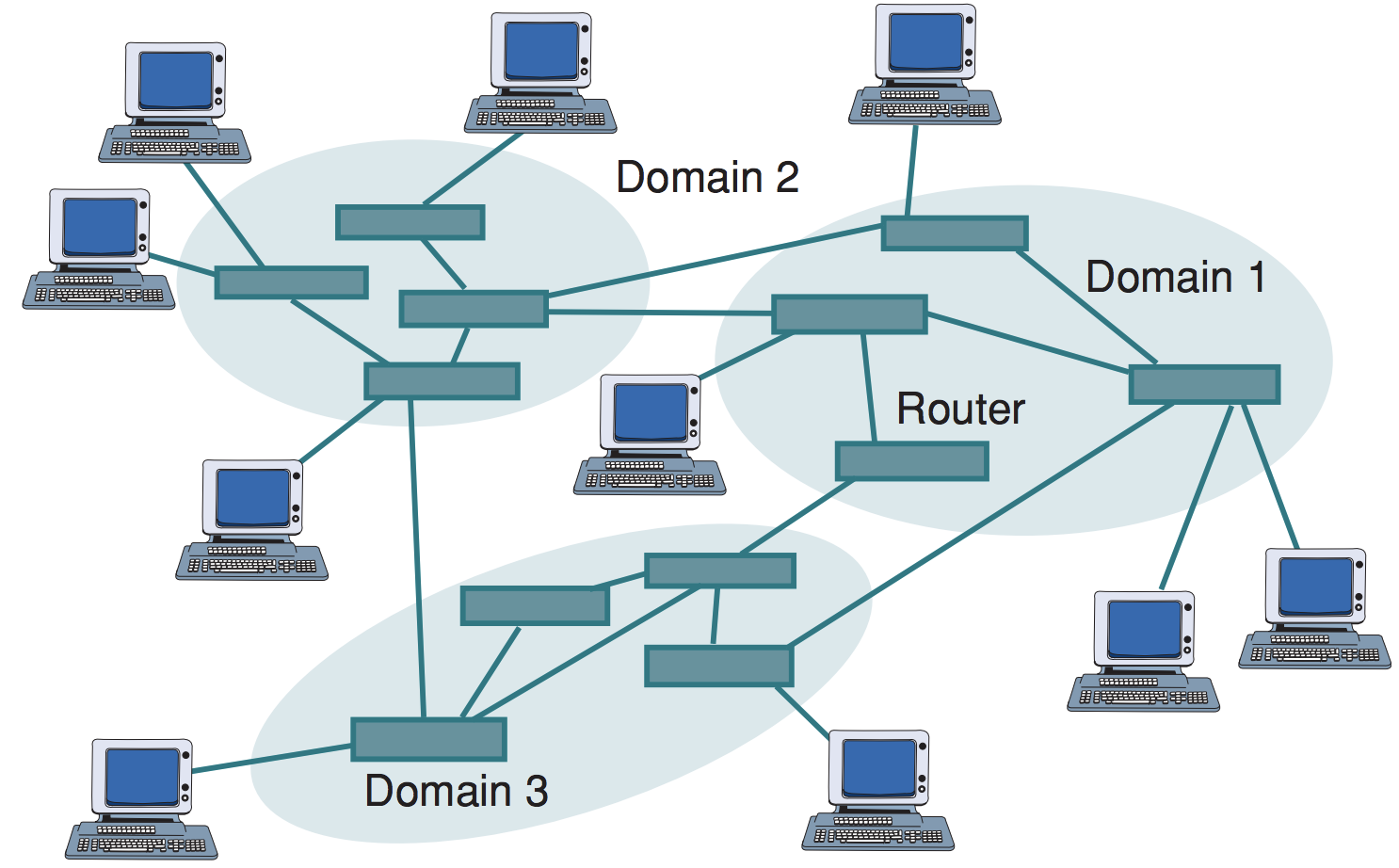
In recent years, digital currency electronic payment has become more popular, and hence, many countries and companies are committed to strengthening security in digital payments to gain customer’s confidence. The number of people sending money using P2P payments was up 116% and the transactions increased by 207% in 2019 compared with the previous year (PYMNTS 2020). P2P networks are also used for sharing electronic files and digital media. Cybersecurity insurance is an indispensable part of the digital currency electronic payment and file-sharing system, especially for the P2P payments/services (Gao et al. 2005; Chandra, Srivastava, and Theng 2010; Kalinic et al. 2019; Lara-Rubio, Villarejo-Ramos, and Liébana-Cabanillas 2020) and the blockchain ecosystem which has a large number of clients and servers. Evaluating the reliability of the P2P systems is an important issue for P2P service providers since scammers can destruct the P2P platform.

Gnutella is an open, decentralized, distributed, P2P search protocol that mainly used to find files (M. Ripeanu 2001). A P2P system can be considered as a cyber network in which individual computers connect directly with each other and share information and resources without using dedicated servers. The nodes in Gnutella perform tasks normally associated with both servers and clients. The nodes provide the client-side interfaces that users can issue queries and accept queries from other users. A synopsis of the network structure of a P2P system is illustrated in Figure 2. For illustrative purposes, in this example, we consider three snapshots of the Gnutella network collected on August 4, 6, and 9, 2002 from the Stanford Network Analysis Project (SNAP) (Leskovec, Kleinberg, and Faloutsos 2007; Matei Matei Ripeanu and Foster 2002). For notation convenience, we denote the Gnutella networks collected on August 4, 6, and 9, 2002 as P2P network by ${\mathbf G_{1}}$, ${\mathbf G_{2}}$, and ${\mathbf G_{3}}$, respectively.

Figure 2.A synopsis of the network structure of a P2P system.

Here, nodes represent hosts in the Gnutella network topology and edges represent connections between the Gnutella hosts. The basic network structure information of the three Gnutella computer networks are presented in Table 1.

In this example, since P2P networks do not have fixed client and servers and the roles of peer nodes would be always changed across different days, the nodes (computers) in the P2P system are not likely to be the same on the three different dates. Therefore, it is reasonable to assume that the P2P network snapshots on August 4, 6, and 9, 2002 are independent and they are three cyber networks with different structures. We are interested in evaluating and comparing the risks of these three networks with different structures for the purpose of determining appropriate cyber insurance policies. For instance, if we find that the three cyber networks are different in terms of risk and reliability, the cyber insurance premium for the network with the highest risk should be higher than the others.

4.1.2. Peer-to-peer network similarity analysis under degree-based attack

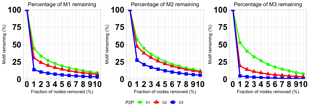
In this subsection, we apply the proposed Wiener process model and hypothesis testing procedures to assess and compare the cyber networks presented in Tables 1 in terms of the robustness and the risk of the cyber networks. The topological features for measuring the risks of the networks are the 4-node network motifs $M_1$, $M_2$, and $M_3$ presented in Figure 1. We remove the nodes in the cyber network based on the degree sequence of the graph (i.e., degree-based attacks), where the degree of a node in a graph is the number of edges that are connected to the node. In other words, the node with the largest degree will get removed first, and the counts of 4-node motifs are obtained when 1%, 2%, …, 10% of the nodes are removed. Figure 3 shows the dynamics of the degradation (in percentages) of the three 4-node motifs under degree-based attacks with $\mathcal{K} = 11$ observation points (including the initial status).

Figure 3.The dynamics of the degradation (in percentages) of the three 4-node motifs of the three networks $\text{G}_{1}, \text{G}_{2}$, and $\text{G}_{3}$ under degree-based attacks with $\mathcal{K}={11}$ observation points.

Following the notation defined in Section 3, $y_{i,j,k}$ corresponds to the counts of the 4-node motif $M_{j}$ $(j=1,2,3)$ when $k\%$ $(k = 0, 1, 2, \ldots, 10)$ of the nodes are removed based on degree-based attack in cyber network ${\mathbf G_{i}}$ ($i = 1, 2, 3$), and $\pmb{x}_{i,k} = (x_{i,1,k},x_{i,2,k}, x_{i,3,k})^{\prime} \in \mathbb{R}^{3}$ is a three-dimensional vector of random variables, where $x_{i,j,k} = (y_{i,j,k} - y_{i,j,k+1})/y_{i,j,0}$, $i = 1, 2, 3$; $j = 1, 2, 3$; $k = 0, 1, 2, \ldots, 10$ is assume to follow a trivariate normal distribution with mean vector $\pmb{\mu}_i$ and variance-covariance $\pmb{\Sigma}_i$.

For the Gnutella computer networks, the MLEs of the drift parameter $\pmb{\mu}_{i} = (\mu_{i1}, \mu_{i2}, \mu_{i3})'$ and the diffusion coefficient $\pmb{\Sigma_{i}} = (\sigma_{i,jj'})_{j, j' = 1, 2, 3}$ for networks ${\mathbf G_i}$ and ${\mathbf G_{\text{Enron}, i}}$, $i = 1, 2, 3$ under degree-based attack are presented in Table 2, where $j, j' = 1, 2, 3$ corresponding to the three 4-node motifs $M_{1}$, $M_2$, and $M_{3}$, respectively. The observed values of the test statistics and the corresponding $p$-values based on Procedures A, B1 and B2 for the pairwise comparisons of the networks $\{{\mathbf G_1}, {\mathbf G_2}, {\mathbf G_3}\}$ are presented in Tables 3. The number of bootstrap samples used in Procedure A and Procedure B2 is $B = 500$.

Considering statistical significance at 5% level and compensating for multiple comparisons by using the Bonferroni correction (Bonferroni 1936), the $p$-values presented in Table 3 that are smaller than $0.05/3 \approx 0.01667$ are highlighted in bold to indicate the cases that the null hypothesis in (6) is rejected. From Table 3, we can see that all the three proposed testing procedures (Procedures A, B1, and B2) show that networks ${\mathbf G_1}$ and ${\mathbf G_3}$ are different in the resilience/risk levels, while networks ${\mathbf G_1}$ and ${\mathbf G_2}$ have no significant difference in the resilience/risk levels at the overall 5% significance level. For the comparison between networks ${\mathbf G_1}$ and ${\mathbf G_2}$, although the $p$-value obtained from Procedure A is greater than the adjusted nominal significance level 0.01667, the small $p$-values from the three test procedures suggests that networks ${\mathbf G_1}$ and ${\mathbf G_2}$ are different in terms of the resilience/risk levels.

From the estimates of the drift parameters presented in Table 2, we observe that ${\hat \mu}_{3j} > {\hat \mu}_{2j} > {\hat \mu}_{1j}$ for $j = 1, 2, 3$, which indicates that the functionality of network ${\mathbf G_1}$ drops slower than networks ${\mathbf G_2}$ and network ${\mathbf G_3}$ subject to the degree-based attacks. In other words, the smaller the values of ${\hat \mu}_{ij}$, the more robust (smaller the risk of) the P2P network. Thus, the results of the analysis based on the proposed methodologies suggest that network ${\mathbf G_1}$ is the most reliable network among the three networks while networks ${\mathbf G_2}$ and ${\mathbf G_3}$ have similar risk levels. These conclusions agree with the observations obtained by looking at the graphs in Figure 3.

In this example, we can see that the proposed methodologies can qualify and compare the risks of different complex networks by using the $p$-values of the hypothesis testing procedures as $p$-value is in (0, 1), and the model parameter estimates. This information can be used in determining the premium of cybersecurity insurance. For example, based on the results in this example, the cybersecurity insurance premium for network ${\mathbf G_1}$ should be lower than the premiums for networks ${\mathbf G_2}$ and ${\mathbf G_3}$ after adjusting for the sizes of those networks and other factors. In the next subsection, we construct concrete scenarios to illustrate how the proposed methodologies can be used to qualify the financial loss due to attack.

4.1.3. Actuarial Applications

In order to help the readers to understand how the proposed model and methods can be used in actuarial science to determine the premium for cybersecurity insurance, we construct several synthetic scenarios to illustrate the effectiveness of our proposed procedures and the role of network motifs on the resilience aspects of financial networks. Suppose each network $\mathbf G_i$ $(i = 1, 2, 3)$ described in Section 4.1.1 corresponds to a company providing P2P financial services and losing a network motif in the P2P network (i.e., a higher-order subgraph in the network) due to cyber-attack translates into a monetary loss to the company. For illustrative purposes, we simplify the problem by considering that the premium of cybersecurity insurance is determined based on (i) the size of the P2P network (the larger the network, the higher the premium); (ii) the cost of losing a network motif in the P2P network (the higher the cost of losing a network motif, the higher the premium); and (iii) the resilience/risk of the P2P network (the higher the risk, the higher the premium).

For the size of the P2P network, we assume that the premium is proportional to the number of nodes in the network. We further assume that the 4-node motifs $M_{1}$, $M_{2}$, and $M_{3}$ carry the same weight, but the cost incurred by losing a motif in the P2P network, which can be viewed as a group of customers and transactions, can be different for the three companies. We denote the cost of losing a motif in the P2P network for company with network $\mathbf G_i$ as $\mathcal{C}_i$, $i = 1, 2, 3$.

For the case that there is no information on the resilience/risk levels of the three P2P networks, if the premium for company with network $\mathbf G_3$ with 8114 nodes is $P₃, then the premium for company with network $\mathbf G_1$ with 10876 nodes can be determined as

$$\begin{aligned} \$P_{1} = \$P_{3} \times \left(\frac{10876}{8114} \right) \left(\frac{\mathcal{C}_1}{\mathcal{C}_3} \right), \end{aligned}$$

and the premium for company with network $\mathbf G_2$ with 8717 nodes can be determined as

$$\begin{aligned} \$P_{2} = \$P_{3} \times \left(\frac{8717}{8114} \right) \left(\frac{\mathcal{C}_2}{\mathcal{C}_3} \right). \end{aligned}$$

Here, the values $(10876/8114)$ and $(8717/8114)$ can be viewed as the factor adjusted for the size of the network, and the values $(\mathcal{C}_1/\mathcal{C}_3)$ and $(\mathcal{C}_2/\mathcal{C}_3)$ can be viewed as the factor adjusted for the cost of losing a network motif in the P2P network.

The methodologies proposed in this paper can provide information on the resilience/risk levels of the three P2P networks by comparing the resilience/risk of these networks statistically which will lead to a more realistic approach to determining the premium of cybersecurity insurance. Specifically, based on the proposed model and methods, the results suggest that network $\mathbf G_1$ is significantly more reliable than networks $\mathbf G_2$ and $\mathbf G_3$, and there is no significant difference between the risk levels of networks $\mathbf G_2$ and $\mathbf G_3$. Based on this information, we can conclude that the premium for the company with network $\mathbf G_1$ should be $$\begin{aligned} \$P_{1} < \$P_{3} \times \left(\frac{10876}{8114} \right) \left(\frac{\mathcal{C}_1}{\mathcal{C}_3} \right). \end{aligned}$$

To obtain a factor that adjusted for the resilience/risk of the P2P network, based on the proposed methodologies in this paper, one possible way is to utilize the estimates from Table 2 by incorporating the decay rates. For example, from Table 2, we can obtain the average decay rate (i.e., average drift parameters), $\bar{\mu} = ({\hat \mu}_{1} + {\hat \mu}_{2} + {\hat \mu}_{3})/3$, for companies with networks $\mathbf G_1$ and $\mathbf G_3$ as ${\bar \mu}^{(1)} = 0.23903$ and ${\bar \mu}^{(3)} = 0.3764$, respectively. Then, we can consider the factor $({\bar \mu}^{(1)}/{\bar \mu}^{(3)}$) to adjust the premium for company with network $\mathbf G_1$ relative to the premium for company with network $\mathbf G_3$. Note that other functions based on the estimates of the proposed modified Wiener process model can be used to construct a reasonable factor here.

The illustration here shows that the network motifs and our proposed statistical procedures can be applied in actuarial science with some reasonable explanations. In real practical applications of determining insurance premium, other factors that are relevant to cybersecurity insurance premium such as the country of the company providing P2P financial services registered in, losses covered/excluded by the insurance policy, security measures of the company, etc., should be considered (Romanosky et al. 2019).

4.2. Enron email network

4.2.1. Background of Enron email network

In the past few years, business email compromise (BEC) becomes one of the top cyber threats. According to the report from (American International Group (AIG) 2019), 23% of its 2018 cyber insurance claims in Europe, Middle East, and Africa (EMEA) region were BEC related. In this example, we consider the Enron email network data collected by the Cognitive Agent that Learns and Organizes (CALO) Project (Klimt and Yang 2004) which consists of more than half a million emails with 150 users sent over the period from May 1999 to July 2001. A node in the Enron email network represents an email address and an edge represents communication between two email addresses, i.e., there exists an edge between node $i$ and node $j$ if at least one email was sent in between email address $i$ and email address $j$. We define the Enron email network as an undirected graph ${\mathbf G_{\text{Enron}}} = (V_{\text{Enron}}, E_{\text{Enron}})$, where $V_{\text{Enron}}$ is a finite set of $|V_{\text{Enron}}| = 36,692$ email addresses and $E_{\text{Enron}}$ is a set of edges (i.e., emails) with $|E_{\text{Enron}}| = 367,662$. A snapshot of the Enron email network is presented in Figure 4.

Figure 4.A snapshot of the Enron email network, where the red nodes represent email addresses and the edge is the email communication between two email addresses.

In order to illustrate our proposed methodologies for evaluating the cybersecurity risk of the Enron email network, we generate three representative subgraphs by sampling $3,000$ nodes from the original Enron email network, i.e., randomly select $3,000$ nodes from the node set $V_{\text{Enron}}$. The numbers of nodes and the numbers of edges of these three subgraphs are presented in Table 4. Furthermore, due to the fact that the email addresses would be different at different time points, we assume that the sampled subgraphs are independent of each other. In a practical application to cybersecurity insurance pricing, we can consider three different companies with the email networks in Table 4 plan to insure their email networks and the insurance company needs to evaluate and compare the risks of these three email networks.

4.2.2. Enron email network security level evaluation under degree-based attack

In the evaluation and comparisons of the risks of the three email networks in Table 4, we consider the dynamics of three $4$-node motif normalized concentrations (i.e., $M_1$, $M_2$, and $M_3$) under degree-based attack. The dynamics of the motifs $M_1$, $M_2$, and $M_3$ under degree-based attack for the three subgraphs ${\mathbf G_{\text{Enron}, 1}}$, ${\mathbf G_{\text{Enron}, 2}}$, and ${\mathbf G_{\text{Enron}, 3}}$ are presented in Figure 5.

Figure 5.The dynamics of the degradation (in percentages) of the three 4-node motifs of the three networks $\mathrm{G}_{\text {Enron,1 }}, \mathrm{G}_{\text {Enron,2 }}$, and $\mathrm{G}_{\text {Enron,3 }}$ under degree-based attacks with $\mathcal{K}=11$ observations points.

For the three subgraphs sampled from the Enron email network, the MLEs of the drift parameter $\pmb{\mu}_{i} = (\mu_{i1}, \mu_{i2}, \mu_{i3})'$ and the diffusion coefficient $\pmb{\Sigma_{i}} = (\sigma_{i,jj'})_{j, j' = 1, 2, 3}$ for networks ${\mathbf G_i}$ and ${\mathbf G_{\text{Enron}, i}}$, $i = 1, 2, 3$ under degree-based attack are presented in Table 5, where $j, j' = 1, 2, 3$ corresponding to the three 4-node motifs $M_{1}$, $M_2$, and $M_{3}$, respectively. From Table 5, the estimates of the drift parameters, $\pmb{\hat \mu}$, are consistent with the observations from the $4$-node motif degradation curves presented in Figure 5. Specifically, except for motif $M_2$, the functionalities of networks ${\mathbf G_{\text{Enron}, 2}}$ and ${\mathbf G_{\text{Enron}, 3}}$ in terms of motifs decline more quickly than than the network ${\mathbf G_{\text{Enron}, 1}}$ as the fraction of nodes were removed. This suggests that the vanishing rates of the motifs are reflecting the robustness (security level) of the email networks. In general, the smaller the values of ${\hat \mu}_{ij}$, the higher the security level of the email network.

For the three Enron email networks, the observed values of the test statistics and the corresponding $p$-values based on Procedures A, B1, and B2 for the pairwise comparisons of the networks $\{{\mathbf G_1}, {\mathbf G_2}, {\mathbf G_3}\}$ are presented in Tables 6. The number of bootstrap samples used in Procedure A and Procedure B2 is $B = 500$. In the analysis of the Enron networks, similar to the analysis of the Gnutella computer networks in Section 4.1.2, we utilize the Bonferroni correction for multiple comparisons, i.e., we can reject the null hypothesis if the corresponding $p$-value is less than $0.01667$ (highlighted in bold in Table 6). From Table 6, the results of the analysis based on the proposed methodologies suggest that networks ${\mathbf G_{\text{Enron}, 1}}$ and ${\mathbf G_{\text{Enron}, 2}}$ have different security levels, ${\mathbf G_{\text{Enron}, 2}}$ and ${\mathbf G_{\text{Enron}, 3}}$ have different security levels, and networks ${\mathbf G_{\text{Enron}, 1}}$ and ${\mathbf G_{\text{Enron}, 3}}$ have similar security levels. Since the smaller the values of ${\hat \mu}_{ij}$, the higher the security level of the email network, based on the estimates from Table 5, we can conclude that ${\mathbf G}_{\text{Enron}, 1}$ and ${\mathbf G_{\text{Enron}, 3}}$ are more robust than $G_{\text{Enron}, 2}$ under the degree-based attacks. These conclusions agree with the observations obtained by looking at the graphs in Figure 5. Based on the results in this analysis, for insurance pricing, the premium for insuring networks ${\mathbf G}_{\text{Enron}, 1}$ and ${\mathbf G}_{\text{Enron}, 3}$ should be similar, while the premium for insuring network ${\mathbf G}_{\text{Enron}, 2}$ should be higher than ${\mathbf G}_{\text{Enron}, 1}$ and ${\mathbf G}_{\text{Enron}, 3}$.

5. Monte Carlo Simulation Studies

In this section, Monte Carlo simulation studies are used to verify the usefulness of the proposed Wiener process model and testing procedures for the similarity of two complex networks in terms of the resilience/risk level. We conduct (i) a simulation study based on a parametric statistical model in Section 5.1; (ii) a simulation study without relying on generating data from a parametric model in Section 5.2; (iii) a sensitivity analysis to evaluate the robustness of the proposed methodologies in Section 5.3. In these simulation studies, we compare the performance of the three proposed testing procedures, Procedure A, Procedure B1, and Procedure B2, for assessing the similarity of different complex networks based on the simulated type-I error rates and the simulated power values.

5.1. Network data generated from a parametric statistical model

In order to evaluate and validate the effectiveness of the proposed methodologies, we consider a simulation study in which the network data are generated based on the Wiener process model in Eq. (1). In this simulation, we assume that there are three different topological features for measuring the risks of two cyber-networks (i.e., $\mathcal{J} = 3$ and $\mathcal{I} = 2$) and these three topological features are observed at $\mathcal{K} = 11$ time points. We are interested in testing the hypotheses in Eq. (6). The topological features for Network 1 and Network 2 in Eq. (6) are simulated from the Wiener process model in Eq. (1) with the following parameter settings based on the networks $\mathbf G_{1}$ and $\mathbf G_{2}$ in the numerical example presented in Section 4:

• Network 1:
  $\pmb{\theta}_1 = (\pmb{\mu}_{1}, \pmb{\Sigma}_{1})$ $\pmb{\mu}_{1} = \begin{pmatrix} 0.2660 \\ 0.2247 \\ 0.3408\\ \end{pmatrix}$ and $\pmb{\Sigma}_{1} = \begin{pmatrix} 0.0388 & 0.0118&0.0128 \\ & 0.0144 & 0.0078\\ & & 0.0171\\ \end{pmatrix};$
  $\pmb{\theta}_1 = (\pmb{\mu}_{1}, \pmb{\Sigma}_{1})$ $\pmb{\mu}_{1} = \begin{pmatrix} 0.2415 \\ 0.2153 \\ 0.2603 \\ \end{pmatrix}$ and $\pmb{\Sigma}_{1} = \begin{pmatrix} 0.0966 &0.0278 & 0.0690 \\ & 0.0320&0.0397 \\ & & 0.1971\\ \end{pmatrix}$.

• Network 2:

  $\pmb{\theta}_{2} = (a \times \pmb{\mu}_{1}, \pmb{\Sigma}_{1})$, where $a = \{0.05, 0.2, 0.4, 0.6, 0.8, 1.0, 1.2, 1.4, 1.6, 1.8, 2.0, 4.0\};$

  $\pmb{\theta}_{2} = (\pmb{\mu}_{1}, a \times \pmb{\Sigma}_{1})$, where $a = \{0.8, 0.6, 0.4, 0.2, 0.05, 1.2, 1.4, 1.6, 1.8, 2.0, 4.0\};$

  $\pmb{\theta}_{2} = (a' + \pmb{\mu}_{1}, \pmb{\Sigma}_{1})$, where $a' = \{0.00, 0.05, 0.10, 0.15, 0.20\}.$

For each combination of the settings for Network 1 and Network 2, we simulated 1,000 sets of experiments and applied the three proposed testing procedures. The number of bootstrap samples used in Procedure A and Procedure B2 is $B = 500$. Considering using 5% significance level, the simulated proportions of the $p$-values less than 0.05 (i.e., rejecting the null hypothesis in (6) at 5% level of significance) are presented in Table 7. Note that when $a = 1.0$ and $a' = 0.0$, the proportions of the $p$-values less than 0.05 are corresponding to the simulated type-I error rates and when $a \not= 1.0$ or $a' \not= 0.0$, the proportions of the $p$-values less than 0.05 are corresponding to the simulated power values.

From the simulation results in Tables 7, we observe that the simulated type-I error rates (i.e., the simulation rejection rates when $a = 1.0$ or $a' = 0.0$) for Procedure A are always controlled under the nominal 5% level for all the settings considered here, while the simulated type-I error rates for Procedures B1 and B2 can be higher than the nominal 5% level. Especially for setting 1(a), Procedure B1 has the simulated type-I error rate of 0.072. For the power of the three proposed procedures, we observe that the power values increases when the simulated settings are further away from the null hypothesis that Network 1 and Network 2 have the same resilience/risk level, i.e., when $a$ increases from 1.0 to 4.0 or $a$ decreases from 1.0 to 0.05, or $a'$ increases from 0.0 to 0.20. These simulation results indicate that the proposed testing procedures can effectively detect the difference in resilience/risk levels between two complex networks. Although Procedure B1 gives larger power values compare to Procedures A and B2 in most cases, it may be due to the inflated type-I error rate. In comparing the power values of Procedures A and B2, the power values of these two procedures are similar, therefore, when taking the ability in controlling type-I error rate, we would recommend using Procedure A based on the simulation results.

5.2. Network data generated from nonparametric resampling of a real network data set

To evaluate the performance of the proposed model and test procedures when the network data are not simulated from a parametric model, we conduct a simulation study based on resampling the real Gnutella P2P network data set presented in Section 4. Based on the analysis of Gnutella P2P network data set presented in Section 4, we observed that there is a significant difference between networks ${\mathbf G_{1}}$ and ${\mathbf G_{3}}$ (i.e., the Gnutella P2P network snapshots on August 4 and 9, 2002, respectively). Therefore, we consider obtaining the simulated networks by resampling from networks ${\mathbf G_{1}}$ and ${\mathbf G_{3}}$ using the breadth-first search (BFS) method (Cormen et al. 2009) as the network sampling approach. The BFS method is known as an important traversing algorithm with many graph-processing applications and has low computational complexity. After deciding the starting target node arbitrarily, the BFS algorithm traverses the graph layerwise in a tree by exploring all of the neighbor nodes at the same layer before moving on to the nodes at a deeper layer until the required number of nodes is reached. In our study, we terminate the graph traversal procedure when we achieved $100 \tau\%$ nodes, where $\tau \in \{0.50, 0.55, \ldots, 0.70\}$. Once again, we are interested in testing the hypotheses in (6). Network 1 and Network 2 in (6) are simulated by resampling the $100 \tau\%$ of nodes as follows:

• Network 1: ${\mathbf G}_{1}$; Network 2: ${\mathbf G}_{1}$;

• Network 1: ${\mathbf G}_{3}$; Network 2: ${\mathbf G}_{3}$;

• Network 1: ${\mathbf G}_{1}$; Network 2: ${\mathbf G}_{3}$.

The simulated rejection rates between two subgraphs under BFS sampling with $100 \tau\%$ nodes, where $\tau \in \{0.50, 0.55, \ldots, 0.70\}$, are presented in Table 8.

From the simulation results in Table 8, we observe that when Network 1 and Network 2 are resampled from ${\mathbf G_{1}}$ and ${\mathbf G_{3}}$, respectively, the three proposed test procedures reject the null hypothesis in (6) more than 90% of times for all the percentages of nodes being resampled considered here. Moreover, the simulated rejection rates increase when the percentage of nodes being resampled increases from 50% to 70%. As we observed in the results presented in Section 4, ${\mathbf G_{1}}$ and ${\mathbf G_{3}}$ are different in terms of their resilience/risk levels. When the two networks are resampled from the same P2P network (i.e., network ${\mathbf G_{1}}$ or network ${\mathbf G_{3}}$), we observed that the simulated rejection rates decrease when the percentage of nodes being resampled increases from 50% to 70%. This agrees with our intuition since the higher the percentage of the nodes being sampled from the same network, the similarity of the two sampled subgraphs is increasing. These simulation results indicate that the proposed testing procedures can effectively detect the difference in resilience/risk levels between two complex networks even when the two networks are not generated from the proposed Wiener process model.

5.3. Sensitivity Analysis

Since the proposed methodologies rely on the Wiener process model, it is important to investigate the sensitivity of the proposed methods when the underlying data generating mechanism deviates from the proposed Wiener process model. For this reason, in this section, we consider a Monte Carlo simulation study in which the simulated datasets are generated from a gamma process model, which is a commonly used model for degradation data analysis.

Following the notation in Section 3.1, we consider $\mathcal{I} = 2$, $\mathcal{J} = 3$ and $\mathcal{K} = 10$ and generate the $\mathcal{J}$-dimensional random vector $\pmb{x}_{i,k} = (x_{i,1,k},x_{i,2,k}, \ldots, x_{i,\mathcal{J},k})^{\prime} \in \mathbb{R}^{\mathcal{J}}$, where $x_{i,j,k} =\log{(y_{i,j,k}/ y_{i,j,k+1})}$, based on a gamma process model in which $x_{i,j,k}$ follows a gamma distribution with shape parameter $\lambda_{i,j} > 0$ and scale parameter $\beta_i >0$ (denoted as $Gamma(\lambda_{i,j}, \beta_i)$). The probability density function of $x_{i,j,k}$ is

$$\begin{aligned} g(x_{i,j,k}; \lambda_{i,j}, \beta_i) &= \frac{\beta_{i}^{\lambda_{i,j}}}{\Gamma(\lambda_{i,j})} x_{i,j,k}^{\lambda_{i,j} - 1} \exp(-\beta_{i} x_{i,j,k}), \\ x_{i,j,k} &> 0, \end{aligned}\tag{11}$$

where $\Gamma(z) = \int_{0}^{\infty} x^{z-1} \exp(-x)~dx$ is the gamma function. For Network $i$ ($i = 1$ and 2), the parameter vector for the gamma process model is $\pmb{\theta}_{i} = (\lambda_{i,1}, \lambda_{i,2}, \lambda_{i,3}, \beta_{i})$. In the simulation study, we consider the following settings for the datasets of Network 1 and Network 2 from the gamma process model:

• Networks 1 and 2 share the same shape parameters but different scale parameter:

  $\pmb{\theta}_1 = (\lambda_{1,1}, \lambda_{1,2}, \lambda_{1,3}, \beta_1)$, where $\lambda_{1,1} = \lambda_{1,2} = \lambda_{1,3} = 0.5$ and $\beta_1 = 0.05$;

  $\pmb{\theta}_2 = (\lambda_{2,1}, \lambda_{2,2}, \lambda_{2,3}, \beta_2)$, where $\lambda_{2,1} = \lambda_{2,2} = \lambda_{2,3} = 0.5$ and $\beta_2 = a \times \beta_1$.

• Networks 1 and 2 share the same scale parameter but different shape parameters:

  $\pmb{\theta}_1 = (\lambda_{1,1}, \lambda_{1,2}, \lambda_{1,3}, \beta_1)$, where $\lambda_{1,1} = \lambda_{1,2} = \lambda_{1,3} = 0.5$ and $\beta_1 = 0.05$;

  $\pmb{\theta}_2 = (\lambda_{2,1}, \lambda_{2,2}, \lambda_{2,3}, \beta_2)$, where $\lambda_{2,1} = \lambda_{2,2} = \lambda_{2,3} = a' + \lambda_{1,i}$ and $\beta_2 = 0.05$.

Based on 1000 simulations with different values of $a$ and $a'$, the simulated rejection rates of Procedures A, B1, and B2 under the proposed modified Wiener process model are presented in Table 9.

From Table 9, we can observe that the three proposed testing procedures, especially Procedure A, under the modified Wiener process model can effectively control the significance levels (i.e., when $a = 1.0$ and $a' = 0.0$) close to the 5% level and provide reasonable power when the two target networks are different in terms of the resilience/risk level even when the underlying data-generating mechanism is not the assumed Wiener process model. Moreover, the power values of these three testing procedures increase with the values of $a$ and $a'$, which indicates that these test procedures can effectively detect the dissimilarity between the two target networks.

6. Concluding Remarks

To comprehend how vulnerable is a cyber or physical network to attacks or failures and to assess the risks of a complex network, in this paper, we propose a statistical approach to assess and understand cyber risk. Specifically, we propose a Wiener process model to model the dynamics of the topological measures of the network under attacks or failures.

To illustrate the utility of the proposed model and testing procedures, we conduct experiments on the Gnutella P2P cyber network and Enron email datasets. Network motifs, which can capture local topological information of a network, are considered as the topological measure in the example. However, other topological measures that can reflect the functionality of the complex network, including global topological measures (e.g., giant component, degree distribution, APL, D, CC, BC, etc.) and local topological features (e.g., Betti numbers, Wasserstein distances, etc.) (Salles and Marino 2011; Kim and Obah 2007; Islambekov et al. 2018) can also be used with the proposed methodologies in this paper. In the practical data analysis, we observe that the proposed methodologies can qualify and compare the risks of different complex networks. Then, we further studied the validity of the proposed methodologies by using two Monte Carlo simulation studies in which the network data are generated from the proposed Weiner process model or resampling from the real Gnutella P2P cyber network data. From the simulation results, we observe that the proposed testing procedures can effectively detect the difference in resilience/risk levels between two complex networks.

To the best of our knowledge, this is the first study that evaluating the resilience/robustness of cyber networks by using a stochastic model with statistical hypothesis testing procedures. The results obtained from the proposed statistical methodologies can provide some important insights to manage and compare the risks of cyber networks and help cybersecurity insurance providers to determine insurance policy and insurance premium. The computer program to execute the proposed methodologies is written in R (R Core Team 2020) and is available from the authors upon request.

Acknowledgement

This research was supported by The Society of Actuaries’ Committee on Knowledge Extension Research and the Casualty Actuarial Society Individual Grant. The authors would like to thank reviewers in the oversight group of the Casualty Actuarial Society for reviewing our manuscript and for their constructive comments and suggestions. The authors are grateful for the two referees and the editor for their helpful and suggestions that improved the manuscript.