1. Introduction
In recent years, risk models have attracted much attention in the insurance business, in connection with the possible insolvency and the capital reserves of insurance companies. The main interest from the point of view of an insurance company is claim arrival and claim size, which affect the capital of the company.
In this paper, we assume that all the processes are defined in a probability space (Ω, F, Pr). Claims happen at the times Ti, satisfying 0 = T0 ≤ T1 ≤ T2 ≤ . . . . The nth claim arriving at time Tn causes the claim size Xn. Now let the constant c represent the premium rate for one unit time; the random variable cTn describes the inflow of capital into the business by time Tn, and describes the outflow of capital due to payments for claims occurring in [0, Tn]. Therefore, the quantity
\[ U_{0}=u, U_{n}=u+c T_{n}-\sum_{i=1}^{n} X_{i} \tag{1.1} \]
is the insurer’s balance (or surplus) at time Tn, n = 1, 2, 3, . . . , with the constant U0 = u ≥ 0 as the initial capital.
We consider the discrete-time surplus process (1.1) in the situation that the possible insolvency (ruin) can occur only at claim arrival times Tn = n, n = 1, 2, 3, . . . . Thus, the model 1.1 becomes
\[ U_{0}=u, U_{n}=u+c n-\sum_{i=1}^{n} X_{i} \tag{1.2} \]
for all n = 1, 2, 3, . . . .
The general approach for studying ruin probability in the discrete-time surplus process is through the so-called Gerber-Shiu discounted penalty function; for example, Pavlova and Willmot (2004), Dickson (2005), and Li (2005b, 2005a). All of these articles study (or calculate) the ruin probability as a function the initial capital u ≥ 0. In this paper, we shall work in the opposite direction, i.e., we study the initial capital for the discrete-time surplus process as a function of ruin probabilities.
2. Main results
Let {Un, n ≥ 0} be a surplus process (as in Section 1) that is driven by the claim process {Xn, n ≥ 1}. We consider the finite-time ruin probabilities of the discrete-time surplus process in Equation (1.2) with the independent and identically distributed (i.i.d.) claim process {Xn, n ≥ 1}. We let be the distribution function of X1, i.e.,
\[ F_{X_{1}}(x)=\operatorname{Pr}\left\{X_{1} \leq x\right\} \tag{2.1} \]
The premium rate c is calculated by the expected value principle, i.e.,
\[ c=(1+\theta) E\left[X_{1}\right] \tag{2.2} \]
where θ > 0 which is the safety loading of insurer.
Let u ≥ 0 be an initial capital. For each n = 1, 2, 3, . . . , we let
\[ \varphi_{n}(u):=\operatorname{Pr}\left\{U_{1} \geq 0, U_{2} \geq 0, U_{3} \geq 0, \ldots, U_{n} \geq 0 \mid U_{0}=u\right\} \tag{2.3} \]
denote the survival probability at the times n. Thus, the ruin probability at one of the time 1, 2, 3, . . . , n is denoted by
\[ \Phi_{n}(u)=1-\varphi_{n}(u) \tag{2.4} \]
Definition 2.1.
Let {Un, n ≥ 0} be a surplus process which is driven by the claim process {Xn, n ≥ 1} and c > 0 be a premium rate. Given α ∈ (0, 1) and N ∈ {1, 2, 3, . . .}. Let an initial capital u ≥ 0, if then u is called an acceptable initial capital corresponding to (α, N, c, {Xn, n ≥ 1}). Particularly, if
\[ u^{*}=\min _{u \geq 0}\left\{u: \Phi_{N}(u) \leq \alpha\right\} \tag{2.5} \]
exists, u* is called the minimum initial capital corresponding to (α, N, c, {Xn, n ≥ 1}) and is written as
\[ u^{*}:=\operatorname{MIC}\left(\alpha, N, c,\left\{X_{n}, n \geq 1\right\}\right) \tag{2.6} \]
2.1. Ruin and survival probability
We define the total claim process by
\[ S_{n}:=X_{1}+X_{2}+\cdots+X_{n} \tag{2.7} \]
for all n = 1, 2, 3, . . . .
Lemma 2.1.
Let N ∈ {1, 2, 3, . . .} and c > 0 be given. If {Xn, n ≥ 1} is an i.i.d. claim process, then is increasing and right continuous and is decreasing and right continuous in u.
Proof. The survival probability at the time N as mentioned in (2.3) can be expressed as follows.
\[ \begin{aligned} \varphi_{N}(u)= & \operatorname{Pr}\left\{S_{1} \leq u+c, S_{2} \leq u\right. \\ & \left.+2 c, \ldots, S_{N} \leq u+N c\right\} \\ = & \operatorname{Pr}\left(\bigcap_{k=1}^{N}\left\{S_{k}-k c-u \leq 0\right\}\right) \\ = & E\left[\bigcap_{k=1}^{\mathbb{I}_{N k-k c-u \leq 0\}}}\right] \\ = & E\left[\prod_{k=1}^{N} \mathbb{I}_{\left\{S_{k}-k c-u \leq 0\right\}}\right] \end{aligned} \tag{2.8} \]
where
\[ \mathbb{I}_{A}(x)=\left\{\begin{array}{l} 1, x \in A \\ 0, x \notin A \end{array}\right. \]
for all A ℝ. Since for all ω ∈ ,
\[ \varphi_{N}(u)=E\left[\prod_{k=1}^{N} \mathbb{I}_{(-\infty, 0]}\left(S_{k}-k c-u\right)\right] \tag{2.9} \]
For each a ∈ ℝ and u ≥ 0, we obtain
\[ \mathbb{I}_{(-\infty, 0]}(a-u)=\left\{\begin{array}{l} 1, {u} \geq {a} \\ 0, {u}<{a} \end{array}\right. \]
then 𝕀(−∞, 0](a − u) is increasing and right continuous in u. This implies that is also increasing and right continuous in u, moreover, this bounding function is identically equal to 1, where ak ∈ ℝ, k = 1, 2, 3, . . . , N. Therefore, by the monotone convergence theorem, we have
\[ \begin{aligned} \lim _{v \rightarrow u^{+}} \varphi_{N}(v) & =\lim _{v \rightarrow u^{+}} E\left[\prod_{k=1}^{N} \mathbb{I}_{(-\infty, 0]}\left(S_{k}-k c-v\right)\right] \\ & =E\left[\lim _{v \rightarrow u^{+}} \prod_{k=1}^{N} \mathbb{I}_{(-\infty, 0]}\left(S_{k}-k c-v\right)\right] \\ & =E\left[\prod_{k=1}^{N} \mathbb{I}_{(-\infty, 0]}\left(S_{k}-k c-u\right)\right] \\ & =\varphi_{N}(u) . \end{aligned} \tag{2.10} \]
Therefore, is increasing and right continuous. Moreover, we can conclude that is decreasing and also right continuous.
Theorem 2.2. Let N ∈ {1, 2, 3, . . .} and c 0 be given. If {Xn, n ≥ 1} is an i.i.d. claim process, then
\[ \lim _{u \rightarrow \infty} \varphi_{N}(u)=1 \text { and } \lim _{u \rightarrow \infty} \Phi_{N}(u)=0 \text {. } \tag{2.11} \]
Proof. First, we will show the following properties
\[ \bigcap_{i=1}^{N}\left\{X_{i} \leq u+c\right\} \subset \bigcap_{i=1}^{N}\left\{S_{i} \leq N u+i c\right\} . \tag{2.12} \]
Let ω {Xi ≤ u + c} be given. For each i ∈ {1, 2, 3, . . . , N}, we have Xi(ω) ≤ u + c and
\[ S_{i}(\omega)=\sum_{k=1}^{i} X_{k}(\omega) \leq i u+i c \leq N u+i c \tag{2.13} \]
That is, ω ∈ {Si ≤ Nu + ic}. Therefore, (2.12) follows. Next, since the process {Xn, n ≥ 1} is i.i.d., then
\[ \operatorname{Pr}\left(\bigcap_{i=1}^{N}\left\{X_{i} \leq u+c\right\}\right)=\prod_{i=1}^{N} \operatorname{Pr}\left\{X_{i} \leq u+c\right\}=(F(u+c))^{N} . \tag{2.14} \]
By Equation (2.8), we have
\[ \varphi_{N}(N u)=\operatorname{Pr}\left(\bigcap_{i=1}^{N}\left\{S_{i} \leq N u+i c\right\}\right) \tag{2.15} \]
By (2.12), (2.14) and (2.15), we obtain
\[ (F(u+c))^{N} \leq \varphi_{N}(N u) \leq 1 \tag{2.16} \]
Since (F(u + c))N → 1 as u → ∞, then → 1 as u → ∞. Thus, we conclude that → 1, and as u → ∞. This is the proof.
Corollary 2.3. Let α ∈ (0, 1), N ∈ {1, 2, 3, . . .} and c 0 be given. If {Xn, n ≥ 1} is an i.i.d. claim process, then there exists ũ ≥ 0 such that, for all u ≥ ũ, u is an acceptable initial capital corresponding to (α, N, c, {Xn, n ≥ 1}).
Proof. We consider by case. Case 1: Since is decreasing, then for all Case 2: By Theorem 2.2 , we have as Thus, there exists such that Since is decreasing, we conclude that for all
2.2. Recursive formula of ruin probabilities
From Theorem 2.2 and Corollary 2.3, we know that the small ruin probability can be controlled by a large initial capital. In this part, we shall describe the upper bound of ruin probability with negative exponential. In order to prove the following lemma, we shall use an equivalent definition of the ruin probability which is given as follows:
\[ \Phi_{n}(u)=\operatorname{Pr}\left(\max _{1 \leq k \leq n}\left(\sum_{i=1}^{k} X_{i}-c k\right)>u\right) \tag{2.17} \]
Theorem 2.4. Let N ∈ {1, 2, 3, . . .}, c 0 and u ≥ 0 be given. If {Xn, n ≥ 1} is an i.i.d. claim process, then the ruin probability at one of the times 1, 2, 3, . . . , N satisfies the following equation
\[ \Phi_{N}(u)=\Phi_{1}(u)+\int_{-\infty}^{u+c} \Phi_{N-1}(u+c-x) d F_{X_{1}}(x) \tag{2.18} \]
where Φ0(u) = 0.
Proof. We will prove (2.18) by induction. We start with n = 1. Since Φ0(u) = 0 for all u ≥ 0, then
\[ \int_{-\infty}^{u+c} \Phi_{0}(u+c-x) d F_{X_{1}}(x)=0 \tag{2.19} \]
This proves (2.18) for n = 1. Now assume that (2.18) holds for n = k ≥ 1. Then
\[ \begin{aligned} \Phi_{k+1}(u)= & \operatorname{Pr}\left(\max _{1 \leq s \leq k+1}\left(\sum_{i=1}^{n} X_{i}-c n\right)>u\right) \\ = & \operatorname{Pr}\left(X_{1}-c>u\right) \\ & +\operatorname{Pr}\left(\max _{2 s n s k+1}\left(X_{1}+\sum_{i=2}^{n} X_{i}-c n\right)>u, X_{1} \leq u+c\right) \\ = & \Phi_{1}(u)+\int_{-\infty}^{u+c} \operatorname{Pr}\left(\max _{1 s n \leq k}\left(x+\sum_{i=2}^{n} X_{i}-c n\right)>u\right) \\ & d F_{X_{1}}(x) \\ = & \Phi_{1}(u)+\int_{-\infty}^{u+c} \operatorname{Pr}\left(\max _{2 s n s k+1}\left(\sum_{i=2}^{n} X_{i}-c(n-1)\right)\right. \\ & >u+c-x) d F_{X_{1}}(x) \\ = & \Phi_{1}(u)+\int_{-\infty}^{u+c} \operatorname{Pr}\left(\max _{2 s n s k+1}\left(\sum_{i=1}^{n-1} X_{i}-c(n-1)\right)\right. \\ & >u+c-x) d F_{X_{1}}(x) \\ = & \Phi_{1}(u)+\int_{-\infty}^{u+c} \operatorname{Pr}\left(\max _{1 \leq n s k}\left(\sum_{i=1}^{n} X_{i}-c n\right)\right. \\ & >u+c-x) d F_{X_{1}}(x) \\ = & \Phi_{1}(u)+\int_{-\infty}^{u+c} \Phi_{k}(u+c-x) d F_{X_{1}}(x) . \end{aligned} \]
which proves (2.18) for n = k + 1 and concludes the proof.
Corollary 2.5. Let N ∈ {1, 2, 3, . . .}, c 0 and u ≥ 0 be given. If {Xn, n ≥ 1} is an i.i.d. claim process, then the ruin probability at one of the times 1, 2, 3, . . . , N satisfies the following equation:
\[ \begin{aligned} \Phi_{0}(u) & =0, \Phi_{1}(u)=1-\operatorname{Pr}(X \leq u+c), \Phi_{N}(u) \\ & =\Phi_{N-1}(u)+\Theta_{N}(u) \end{aligned} \tag{2.20} \]
where
\[ \Theta_{N}(u)=\int_{-\infty}^{u+c}\left(\int_{-\infty}^{u+c-x} \Phi_{N-2}(u+2 c-x-v) d F_{X_{1}}(v)\right) d F_{X_{1}}(x) \]
for all n = 2, 3, 4, . . . .
Proof. Let N ≥ 2, by Theorem 2.4, we obtain
\[ \begin{aligned} \Phi_{N}(u) & =\Phi_{1}(u)+\int_{-\infty}^{u+c} \Phi_{N-1}(u+c-x) d F_{X_{1}}(x) \\ = & \Phi_{1}(u)+\int_{-\infty}^{u+c}\left(\Phi_{N-2}(u+c-x)\right. \\ & \left.+\int_{-\infty}^{u+2 c-x} \Phi_{N-2}(u+2 c-x-v) d F_{X_{1}}(v)\right) d F_{X_{1}}(x) \\ = & \Phi_{1}(u)+\int_{-\infty}^{u+c}\left(\Phi_{N-2}(u+c-x) d F_{X_{1}}(x)\right. \\ & +\int_{-\infty}^{u+c}\left(\int_{-\infty}^{u+2 c-x} \Phi_{N-2}(u+2 c-x-v) d F_{X_{1}}(v)\right) d F_{X_{1}}(x) \\ = & \Phi_{N-1}(u)+\int_{-\infty}^{u+c}\left(\int_{-\infty}^{u+2 c-x} \Phi_{N-2}(u+2 c-x-v) d F_{X_{1}}(v)\right) \\ & d F_{X_{1}}(x) . \end{aligned} \]
This completes the proof.
Corollary 2.6. Let N ∈ {1, 2, 3, . . .} and u ≥ 0. Assume that {Xn, n ≥ 1} is a sequence of exponential distribution with intensity λ 0, i.e., X1 has the probability density function The obtained ruin probability is in the following recursive form
\[ \begin{aligned} \Phi_{0}(u)= & 0, \Phi_{n}(u)=\Phi_{n-1}(u) \\ & +\frac{(u+c) \lambda^{n-1}(u+n c)^{n-2}}{(n-1) !} e^{-\lambda(u+n c)} \end{aligned} \tag{2.21} \]
for all n = 1, 2, 3, . . . , where the initial capital u ≥ 0 and premium rate c E[X1] = 1/λ.
Proof. We will prove (2.21) by induction. We start with n = 1, Φ1(u) = 1 − Pr {X ≤ u + c} = 1 − (1 − =
This proves (2.21) for n = 1. Next we assume that (2.21) holds for n = k ≥ 1. From Theorem 2.2, we have
\[ \begin{aligned} \Phi_{k+1}(u)= & \Phi_{1}(u)+\int_{0}^{u+c} \Phi_{k}(u+c-x) d F_{X_{1}}(x) \\ = & \Phi_{1}(u)+\int_{0}^{u+c}\left(\Phi_{k-1}(u+c-x)\right. \\ & +\frac{(u+2 c-x) \lambda^{k-1}(u+(k+1) c-x)^{k-2}}{(k-1) !} \\ & \left.e^{-\lambda(u+(k+1) c-x)}\right) d F_{X_{1}}(x) \end{aligned} \]
\[ \begin{aligned} = & \Phi_{k}(u)+\int_{0}^{u+c} \frac{(u+2 c-x) \lambda^{k-1}(u+(k+1) c-x)^{k-2}}{(k-1) !} \\ & e^{-\lambda(u+(k+1) c-x)} d F_{X_{1}}(x) \end{aligned} \tag{2.22} \]
and
\[ \begin{aligned} \Theta_{k+1}(u)= & \int_{0}^{u+c} \frac{(u+2 c-x) \lambda^{k-1}(u+(k+1) c-x)^{k-2}}{(k-1) !} \\ = & \frac{e^{-\lambda(u+(k+1) c-x)} e^{-\lambda x} d x}{(k-1) !} \int_{0}^{-\lambda(u+(k+1) c)} \int^{u+c}(u+(k+1) c-x)^{k-2} \\ & (u+(k+1) c-x-(k-1) c) d x \\ = & \frac{\lambda^{k} e^{-\lambda(u+(k+1) c)} \int_{0}^{u+c}}{(k-1) !}\left((u+(k+1) c-x)^{k-1}\right. \\ & \left.+(k-1) c(u+(k+1) c-x)^{k-2}\right) d x \\ = & \frac{(u+c) \lambda^{k}(u+(k+1) c)^{k-1}}{k !} e^{-\lambda(u+(k+1) c)}, \end{aligned} \]
which proves (2.21) for n = k + 1 and completes the proof.
2.3. Existence of minimum initial capital
A quantity α, which was discussed in the previous section, can be described as the most acceptable probability that the insurance company will become insolvent. As a result of Corollary 2.3, we obtain that is a non-empty set. This means that we can always choose an initial capital which makes the value of ruin probability not exceed α. Since the set is an infinite set, then there are many acceptable initial capital corresponding to (α, N, c, {Xn, n ≥ 1}). In this section, we will prove the existence of
\[ \operatorname{MIC}\left(\alpha, N, c,\left\{X_{n}, n \geq 1\right\}\right)=\min _{u \geq 0}\left\{u: \Phi_{N}(u) \leq \alpha\right\} \tag{2.23} \]
Lemma 2.2. Let a, b and α be real numbers such that a ≤ b. If f is decreasing and right continuous on [a, b] and α ∈ [f(b), f(a)], then there exists d ∈ [a, b] such that
\[ d=\min \{x \in[a, b]: f(x) \leq \alpha\} . \tag{2.24} \]
Proof. Let
\[ S:=\{x \in[a, b]: f(x) \leq \alpha\} \]
Since α ∈ [f(b), f(a)], i.e., f(b) ∈ α ≤ f(a), then b ∈ S. That is, S is a non-empty set. Since S is a subset of closed and bounded interval [a, b], then there exists d ∈ [a, b] such that d = inf S. Next, we consider by case.
Case 1: d = b. We know that b ∈ S, thus b = min S.
Case 2: a ≤ d b. Since d = inf S, then there exists dn ∈ S such that
\[ {d} \leq {d}_{n}<{d}+1 / {n} \]
for all n ∈ ℕ. For each n 2/(b − d), we have
\[ {d}<{d}+1 / {n}<{d}+\frac{b-d}{2}=\frac{b+d}{2}<{b} . \]
This means that d + 1/n ∈ (d, b) ⊂ [a, b] for all n 2/(b − d). Since f is decreasing and dn ∈ S, we get
\[ f(d+1 / n) \leq f\left(d_{n}\right) \leq \alpha \]
i.e., d + 1/n ∈ S for all n 2/(b − d). Since f is right continuous at d, we have
\[ f(d)=\lim _{n \rightarrow \infty} f(d+1 / n) \leq \alpha \]
Therefore, d ∈ S, i.e., d = min S. This completes the proof.
Theorem 2.7. Let α ∈ (0, 1), N ∈ {1, 2, 3, . . .}, and c 0. Then there exist u* ≥ 0 such that
\[ u^{*}=\operatorname{MIC}\left(\alpha, N, c,\left\{X_{n}, n \geq 1\right\}\right) \]
Proof. We consider by case. Case 1: we have
\[ \operatorname{MIC}\left(\alpha, N, c,\left\{X_{n}, n \geq 1\right\}\right)=0 \]
Case 2: by Corollary 2.3 , there exists such that i.e., Since is decreasing and right continuous, by Lemma 2.2 there exists such that
\[ u^{*}=\min _{u \in 0, \bar{i}]}\left\{u: \Phi_{N}(u) \leq \alpha\right\}=\min _{u \in 0, \infty)}\left\{u: \Phi_{N}(u) \leq \alpha\right\} \]
That is,
\[ u^{*}=\operatorname{MIC}\left(\alpha, N, c,\left\{X_{n}, n \geq 1\right\}\right) \]
Next, we will approximate the minimum initial capital MIC(α, N, c, {Xn, n ≥ 1}) by applying the bisection technique for the decreasing and right continuous function.
Theorem 2.8. Let α ∈ (0, 1), N ∈ {1, 2, 3, . . .}, and v0, u0 ≥ 0 such that v0 u0. Let and be a real sequence defined by
\[ \left\{\begin{array}{ll} v_{k}=v_{k-1} & \text { and } u_{k}=\frac{u_{k-1}+v_{k-1}}{2}, \\ & \text { if } \Phi_{N}\left(\frac{u_{k-1}+v_{k-1}}{2}\right) \leq \alpha \\ v_{k}=\frac{v_{k-1}+u_{k-1}}{2} & \text { and } u_{k}=u_{k-1}, \\ & \text { if } \Phi_{N}\left(\frac{u_{k-1}+v_{k-1}}{2}\right)>\alpha \end{array}\right. \]
for all k = 1, 2, 3, . . . . If then
\[ \lim _{k \rightarrow \infty} u_{k}=\operatorname{MIC}\left(\alpha, N, c,\left\{X_{n}, n \geq 1\right\}\right) \tag{2.25} \]
and
\[ 0 \leq u_{k}-\operatorname{MIC}\left(\alpha, N, c,\left\{X_{n}, n \geq 1\right\}\right) \leq \frac{u_{0}-v_{0}}{2^{k}} \tag{2.26} \]
for all k = 1, 2, 3, . . . .
Proof. Obviously, is decreasing and is increasing, moreover, vk ≤ uk for all k = 1, 2, 3, . . . . Thus, and are convergent. Since
\[ 0 \leq u_{k}-v_{k}=\left(u_{0}-v_{0}\right) / 2^{k} \rightarrow 0 \text { as } k \rightarrow \infty, \]
then there exists u* ∈ [v0, u0] such that
\[ \lim _{k \rightarrow \infty} u_{k}=\lim _{k \rightarrow \infty} v_{k}:=u^{*} \tag{2.27} \]
Since is decreasing and for all then for all Since is right continuous and for all then
\[ \Phi_{N}\left(u^{*}\right)=\lim _{k \rightarrow \infty} \Phi_{N}\left(u_{k}\right) \leq \alpha \tag{2.28} \]
Therefore,
\[ u^{*}=\operatorname{MIC}\left(\alpha, N, c,\left\{X_{n}, n \geq 1\right\}\right) . \tag{2.29} \]
For each k = 0, 1, 2, . . . , we have vk ≤ u* ≤ uk. This implies that
\[ \begin{array}{c} 0 \leq u_{k}-u^{*} \leq u_{k}-u^{*}+u^{*}-v_{k} \\ =u_{k}-v_{k}=\frac{u_{0}-v_{0}}{2^{k}} . \end{array} \tag{2.30} \]
This completes the proof.
2.4. Numerical results
We provide numerical illustrations of the main results. We approximate the minimum initial capital of the discrete-time surplus process (1.2) by using Theorem 2.8 in the case of {Xn, n ≥ 1} a sequence of i.i.d. exponential distribution with intensity λ = 1, by choosing model parameter combinations θ = 0.10 and 0.25, i.e., c = 1.10 and c = 1.25, respectively; and α = 0.1, 0.2, and 0.3.
Table 1 shows the approximation of MIC(α, N, c, {Xn, n ≥ 1}) with u25 as mentioned in Theorem 2.8, choosing v0 = 0 and u0 = 20, and is computed from the recursive form (2.21).
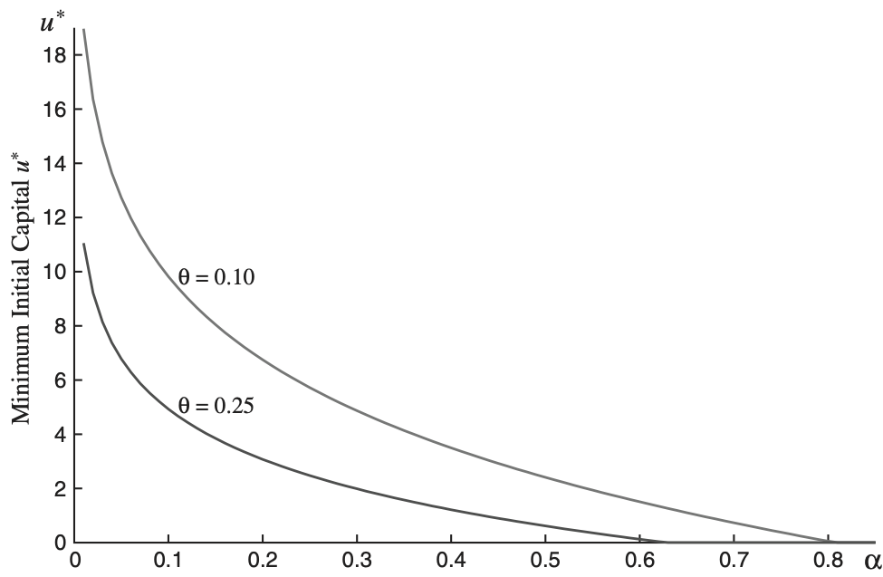
Figure 1 shows the approximation of MIC(α, N, c, {Xn, n ≥ 1}) for the various values of α with u25 as mentioned in Theorem 2.8. Here we choose v0 = 0, u0 = 20, and parameter combinations θ = 0.10, θ = 0.25, i.e., c = 1.10 and c = 1.25, respectively.
_in_the_discrete-time_surplus_process.png)