Pricing in a Competitive Insurance Market Driven by Fractional Noise

undefined

1. Introduction

The pricing process is a critical matter for any insurance company. Traditionally, the specific problem is tackled within a static framework, that is, the pure premium is set equal to the expected claims of a certain time period, in addition to a margin characterized as safety loading. A further increase due to expense and profit provisions is also added. Hence, the following structure holds for the calculation of the gross premium (Figure 1).

Under the static approach, the safety loading is determined on a constant basis, which ultimately results in an explosive level of surplus. The dynamic setting proposed by Lundberg (1903) and Cramer (1930) at the beginning of the twentieth century provided the necessary theoretical framework for the solution of this undesirable problem of the explosive surplus. Under this dynamic approach, Borch (1967) considered a flexible model where the safety loading is partially or fully controlled, resulting in a stable state for the surplus level. An insurance company may simultaneously stabilize its surplus level while also following potential underwriting cycles of the total claims. Following the approach of Borch (1967), Vandebroek and Dhaene (1990), Martin-Löf (1994), Norberg (1999), and Zimbidis (2008) have provided further insights into the problem of premium control. The drawback of this approach is the resulting variable premium that may upset the client’s behavior. Premium changes (especially increases) normally lead clients to investigate the market and, perhaps, change their policy. Of course, the decision for a change is more frequent (and easier) in the general insurance market where we have annual renewable policies.

Therefore, a more sophisticated dynamic model (where the premium is partially or fully controlled) should also include the concept of a demand function that determines the volume of business under the different levels of premium. Such a model had been initially proposed by Taylor (1986) in a discrete framework and revisited in a continuous framework by Emms, Haberman, and Savoulli (2007). The demand functions appearing in those works all contain the concept of the “average premium of the market,” which is modeled either on a deterministic basis or stochastically via the standard Brownian motion.

In this paper, we adopt the pricing framework model of a competitive market using the fractional Brownian motion as a modeling tool for the movement of the market’s average premium. This is supported by the empirical evidence of the data gathered from the Greek motor insurance market within the last decade.

This paper is organized as follows. In Section 2, we briefly discuss the concept of the competitive insurance markets. Section 3 provides a short background on fractional Brownian motion. In Section 4, we formulate the general model, and in Section 5 we solve a special case. Section 6 contains some insights into the structure of the Greek motor insurance market, identifies the phenomenon of long-range dependency, and provides a short numerical application. In Section 7, we add some final comments.

2. Competitive insurance markets

The structure of a competitive insurance market can be extremely complicated. Here, we consider only the effect of the premium relativities, and how these quantities determine the market share of each company. We assume that the volume of business is determined via the function

$$V(t)=f(p(t), \bar{p}(t), \tilde{\psi}(t)), \tag{1}$$

where $V(t)$ is the volume of business, $p(t)$ is the premium rate of the company, $\bar{p}(t)$ is the market’s average premium rate, and $\tilde{\psi}(t)$ is a vector of different parameters (e.g., money spent in the advertisement campaign of the company) that affects the market share of the company at time $t$. A more theoretical approach for market description (states and movements) may be found in Figure 2 that provides a simplified version of the respective payoff matrix.

State A: A is the stable state of the system. Every company, and consequently the whole market, retains high constant premium rates within profitable levels. The market shares of all companies are also more or less constant.

Out → A : A new company enters the market.

A → B: The new company (or one of the previously existing companies of the market) is trying to enhance its market share by cutting its prices. The company may achieve this goal and moves the system into State B.

State B: B is the unstable state of the system. The other companies either slowly or quickly understand the loss and plan their reactions.

B → C: All the companies (and consequently the whole market) drop their prices to regain their market share and secure their position.

State C: C is a partially stable state of the system. The companies will continue to charge low premium rates, insofar as their financial strength permits them to.

C → Out: A company is not strong enough to maintain the low premium rates and either goes bankrupt or (trying unsuccessfully to increase its rates while others retain the low ones) goes out of the market.

C → D: A company (probably one of the major ones) increases its rates, trying to return to profitable levels. The company manages to retain its clients, although the total market suggests lower premium rates.

State D: D is a partially stable–unstable state of the system. The market will continue charging low premium rates for a while, while a few companies charge correct premium rates and make profits.

D → A: All the companies increase their premium rates up to profitable levels.

Generally speaking, a company’s premium decrease (compared with the market’s average premium) will raise the company’s market share and vice versa; that is, for a constant value of p(t), we obtain

$$\lim _{p(t) \rightarrow \infty} f(p(t), \bar{p}(t), \tilde{\psi}(t))=0 \tag{2}$$

while

$$\lim _{p(t) \rightarrow 0} f(p(t), \bar{p}(t), \tilde{\psi}(t))=E, \tag{3}$$

where $E$ corresponds to the total market.

Now, the fundamental question is why should long-range dependency exist in the process that describes the market’s average premium within an insurance market? Suppose an insurance company makes the first move by decreasing its premium and consequently lowering the market average. Then the other companies will do the same to retain their clients, and the average will move down even more. So, we should expect to observe a “persistency” phenomenon (and not an anti-persistency phenomenon) and therefore a value for the Hurst exponent within the interval (½, 1).

3. Fractional Brownian motion—Theory and evidence

Fractional Brownian motion (fBm) has proved to be quite an efficient tool for modeling complicated systems in many scientific areas, such as finance, biology, image processing, and network traffic in the last two decades. Kolmogorov (1940) initially introduced such a stochastic motion, while Mandelbrot and Van Ness (1968) discussed the physical derivation of this process. The climatologist Hurst (1951) observed the long-range dependency property within the data of the yearly water flows of the Nile River. In this section, we provide a short note for the respective theoretical framework required for fBm, as well as a special final subsection that deals with the estimation procedure of the basic index of this process. This basic index is named Hurst exponent after the climatologist Hurst.

3.1. The general theoretical framework

In the rest of this paper, all random variables and processes are defined on a given complete probability space $(\Omega, \Phi, \Pi^H)$, where $\Omega$ is the sample space, $\Phi$ is the σ-algebra generated as the $\Pi^H$ completion of the natural filtration of the $W^H$ process, and $\Pi^H$ is the respective probability measure.

The $W^H = \{ W^H (t); t \geq 0 \}$ process is assumed to be a fractional Brownian motion with a Hurst exponent $H$, where $0.5 \leq H \leq 1$ and may be regarded as the fractional time derivative of the Gausssian white noise. The basic properties of such a process are

1. $\Pr \lbrack W^H (0) = 0 \rbrack = 1$;

2. $W^H (t)$ is an $\Phi$ - measurable function (random variable) for each $t \in \Re_+$, with $\text{E} \lbrack W^H (t) \rbrack = 0$;

3. $\text{E} \lbrack W^H (s) \cdot W^H (t) \rbrack = \frac{1}{2} \lbrack s^{2H} + t^{2H} - | s - t |^{2H} \rbrack$ for any $s,t \in \Re_+$ .

The expectation operator E[ ] is applicable using the $\Pi^H$ probability measure.

Using the properties mentioned here and Kolmogorov’s continuity criterion, we can determine that fractional Brownian motion has a version with continuous sample paths with probability one, but these paths are nowhere differentiable. Further, we should state that fBm is a Gaussian process, self-similar with stationary increments exhibiting long-range dependence.

Obviously, for the special value of the Hurst exponent H = 0.5, the process is reduced to the standard Brownian motion. For H ≠ 0.5 the process $\Omega^H$ is not a Markovian, martingale, or even semi-martingale process. Therefore, the classical stochastic calculus, the theory of integration, and the other powerful tools of standard stochastic analysis are not (yet!) available, although there are certain simple integral transformations connecting the fractional Brownian motion with standard Brownian motion (Norros, Valkeila, and Virtamo 1999).

$$W^{H}(t)=c(H) \int_{\Re}\left[\left((t-x)^{+}\right)^{H-\frac{1}{2}}-\left((-x)^{+}\right)^{H-\frac{1}{2}}\right] d W(t) . \tag{4}$$

Significant research efforts have been made in two directions:

1. Stochastic integration, that is, to establish an analogous theory of stochastic integration retaining the desirable properties of the Ito integral as the zero mean property (see the references in Section 3.2), and

2. Stochastic control, that is, to launch a concrete general theory for the control and optimization of systems driven by fractional Brownian motion (Kleptsyna, Le Breton, and Viot 2003; Hu and Zhou 2005).

3.2. Stochastic integration for the fBm

The first attempts by Lin (1995) and Dai and Heyde (1996) to define an integral with respect to the fractional Brownian motion with a Hurst exponent H > 0.5 resulted in a stochastic integral which does not posses the zero-mean property. Their approach was rather standard, defining the stochastic integral as the limit of Riemannian sums in L²(Ω; ℜ ) – the space of real-valued square integrable functions. As the absence of zero-mean property is not convenient either for the theoretical development or practical (usually financial) applications, new proposals have been raised (Duncan, Hu, and Pasik-Duncan 2000; Carmona and Coutin 2003). These alternative proposals have been developed using the techniques of Malliavin calculus and Wick product.

Hence, given a time interval [0,T], a function F continuously differentiable that satisfies an exponential growth condition and H > 0.5, we can define the Wick stochastic integral with respect to fractional Brownian motion as follows:

$$\begin{array}{l} \int_{0}^{T} F\left(W^{H}(t)\right) \diamond d W^{H}(t) \\ \quad=\int_{0}^{T} F\left(W^{H}(t)\right) d W^{H}(t)-H \int_{0}^{T} F^{\prime}\left(W^{H}(t)\right) t^{2 H-1} d t . \end{array}$$

The $\diamond$ symbol corresponds to the Wick product, while $\int_{0}^{T} F\left(W^{H}(t)\right) d W^{H}(t)$ is the path-wise Riemann-Stielges integral. This is well defined for H > 0.5, given that F is continuously differentiable. Moreover, the following result holds if Φ′ = F:

$$\int_{0}^{T} F\left(W^{H}(t)\right) d W^{H}(t)=\Phi\left(W^{H}(T)\right)-\Phi(0). \tag{5}$$

It is proved that the Wick stochastic integral described here has the zero-mean property (Duncan, Hu, and Pasik-Duncan 2000).

3.3. Stochastic control for linear systems driven by fractional noises

We assume the general format of a linear stochastic controlled differential equation,

$$\begin{align} dx(t) &= (A(t)x(t) + B(t)u(t))dt \\ &\quad + (C(t)x(t) + D(t)u(t))dW^H (t), \end{align} \tag{6}$$

where $x(t)$ is the state variable, $u(t)$ is the control variable, $A(t)$, $B(t)$, $C(t)$, and $D(t)$ are given essentially bounded deterministic (matrix-valued) functions of $t$ and $W^H = \{ W^H (t); t \geq 0 \}$, is a fractional Brownian motion with a Hurst exponent $H$.

Then, we denote with $Y^H$ the class of $(\Phi_t^H)$- adapted processes u, where u = {u_t, t ≥ 0}, for which the system admits a unique strong solution $x_u$. Of course, then $x_u$ is an $(\Phi_t^H)$-adapted process. Actually, for control purposes, we are interested only in closed-loop policies. Therefore, we initiate a sub-class of admissible controls as the class $Y_{\text{ad}}^H$ of those u’s in $Y^H$ which are $(\Phi_{t,u}^H)$-adapted processes where $(\Phi_{t,u}^H)$ is the natural filtration of the corresponding state process $x_u$. Then, the pair $(u, x_u)$ is called an admissible pair. Now we introduce the functional,

$$\begin{align} J(u)&:=J\left(x_0, u\right)\\ &\ =E\Biggl[\int_0^T\left(x^*(t) Q(t) x(t)+u^*(t) R(t) u(t)\right) d t\\ &\hspace{12em}+x^*(T) G\ x(T)\Biggr], \end{align} \tag{7}$$

where $Q(t)$, $R(t)$ and $G$ are positive definite matrices.

Hence, the pair $(u^{opt}, x_u^{opt})$ is defined as the optimal pair if

$$J\left(u^{o p t}\right)=\inf \left\{J\left(x_{0}, u\right) ; u \in U_{a d}\right\}, \tag{8}$$

while the $J(u^{opt})$ is established as the optimal cost for the system.

Regarding the theoretical results with respect to the derivation of the optimal solution $u^{opt}$ for the system described by expressions (6) and (7), we have the following basic theorem.

 

Theorem 3.1. The optimal solution for the system of expressions (6) and (7) is determined via the feedback formula

$$u^{o p t}(t)=K(t) \cdot x(t) \tag{9}$$

where $K(t) = (K_1 (t), \ldots, K_m (t))^*$ satisfies the equation given here

$$\begin{array}{l} K^{*}(t) \cdot R(t) \cdot \Theta(t) \\ \quad+B(t) \cdot \int_{t}^{1} \Theta(s)\left(Q(s)+K^{*}(s) \cdot R(s) \cdot K(s)\right) d s \\ \quad+D(t) \cdot \int_{T}^{T} \int_{0}^{S} \Theta(s) \cdot \phi\left(s^{\prime}, t\right) \\ \hspace{8em}\cdot\left(C\left(s^{\prime}\right) +D\left(s^{\prime}\right) \cdot K\left(s^{\prime}\right)\right) ^*\left(Q(s)\\ \hspace{6em}+K^{*}(s) \cdot R(s) \cdot K(s)\right) d s^{\prime} d s \\ \quad+G \cdot \Theta(T)\left[B(t)+D(t) \int_{0}^{T} \phi\left(s^{\prime}, t\right)\left(C\left(s^{\prime}\right)\\ \hspace{12em} +D\left(s^{\prime}\right) \cdot K\left(s^{\prime}\right)\right) ^* d s^{\prime}\right]=0, \\ \text { a.e. } s \in[0, T] \end{array} \tag{10}$$

while

$$\phi(s, t)=H(2 H-1)|s-t|^{2 H-2} \tag{11}$$

$$\begin{align} \Theta(t)&=x_{0}^{2} \cdot E\Biggl\{\exp \biggl[2 \int_{0}^{t}(A(s)+B(s) K(s)) d s \\ &\hspace{5em}+\int_{0}^{t} \int_{0}^{t} \phi\left(s, s^{\prime}\right)(C(s)+D(s) K(s)) \\ &\hspace{7em} \cdot\left(C\left(s^{\prime}\right)+D\left(s^{\prime}\right) L\left(s^{\prime}\right)\right) ^* d s d s^{\prime}\biggr]\Biggr\}. \end{align} \tag{12}$$

Proof: Refer to the 2nd special case of Theorem (4.1) of Hu and Zhou (2005).

3.4. Estimation of the Hurst exponent

Given the data of a time series, the Hurst exponent H may be regarded as a measure of smoothness and is defined as

$$H=\frac{\ln (R / S)}{\ln (T)}, \tag{13}$$

where $R$ is the respective range, $S$ is the standard deviation, and $T$ is the duration of the sample data. Additionally, the Hurst index $H$ is directly related with the fractal dimension of these data and the following equation holds:

$$H=\boldsymbol{E}+1-\boldsymbol{D} \tag{14}$$

where $\boldsymbol{E}$ is the Euclidean dimension (e.g., $\boldsymbol{E} = 0$ for a point, $\boldsymbol{E} = 1$ for a line, $\boldsymbol{E} = 2$ for surface) and $\boldsymbol{D}$ is the fractal dimension of the sample data.

Regarding the procedure for the estimation of the Hurst exponent, we describe the algorithm based on the rescaled range.

Consider the data series ɸ₁, ɸ₂, . . . ɸ_n. Then we follow the steps described here.

Step 1. Calculate the sample mean and standard deviation

$$\bar{\varphi}(\mathrm{n})=\frac{1}{\mathrm{n}} \sum_{i=1}^{\mathrm{n}} \varphi_{\mathrm{i}} \quad\quad \mathrm{S}(\mathrm{n})=\left[\frac{1}{\mathrm{n}-1} \sum_{i=1}^{\mathrm{n}}\left(\varphi_{\mathrm{i}}-\bar{\varphi}(n)\right)^2\right]^{\frac{1}{2}} .$$

Step 2. Calculate the running sum of the centered observations,

$$\Phi(\kappa)=\sum_{i=1}^{\kappa}\left[\varphi_{\mathrm{i}}-\bar{\varphi}(n)\right] \quad\quad \kappa=1,2, \ldots, \mathrm{n}.$$

Step 3. Calculate the respective range of the data,

$$R(n)=\max _{1 \leq \kappa \leq \text{n}} \Phi(\kappa)-\min _{1 \leq \kappa \leq \text{n}} \Phi(\kappa) .$$

Step 4: The Hurst exponent is defined as $\mathrm{H}(0)=\frac{\ln (R(n) / S(n))}{\ln (n)}$.

Step 5: Split the whole data series in two subseries, $\phi_1, \phi_2, \ldots, \phi_{n_{11}}$ and $\phi_{n_{11}+1}, \ldots, \phi_n$ where $n_{11}=\left[\frac{\mathrm{n}}{2}\right]$, and repeat steps 1–4, estimating the Hurst index that corresponds to data series $\phi_1, \phi_2, \ldots, \phi_{n_{11}}$ defined as H(1,1) and Hurst index that corresponds to data series $\phi_{n_{11}+1}, \ldots, \phi_n$ defined as H(1,2). Then we calculate the mean as

$$H(1)=\frac{H(1,1)+H(1,2)}{2}.$$

Step 6. Continue with a second split and obtain the following four subseries

$$\small \begin{aligned} \varphi_{1}, \ldots \ldots, \varphi_{\mathrm{n}_{21}} \quad \varphi_{\mathrm{n}_{21}+1}, \ldots \ldots, &\varphi_{\mathrm{n}_{11}} \\ & \varphi_{\mathrm{n}_{11}+1}, \ldots \ldots, \varphi_{\mathrm{n} 22} \quad \varphi_{\mathrm{n}_{22}+1}, \ldots \ldots, \varphi_{\mathrm{n}} \end{aligned}$$

where $\mathrm{n}_{21}=\left[\frac{\mathrm{n}_{11}}{2}\right]$ and $\mathrm{n}_{22}=\mathrm{n}_{11}+\left[\frac{\mathrm{n}-\mathrm{n}_{11}}{2}\right]$.

Repeat steps 1–4 for the four subseries and obtain estimations for the Hurst exponent for each subseries,

$$H(2,1), H(2,2), H(2,3) \text { and } H(2,4) \text {, }$$

and finally derive their average,

$$H(2)=\frac{H(2,1)+H(2,2)+H(2,3)+H(2,4)}{4} \text {. }$$

Step 7: Continue splitting the data series up to the level where at least eight data points are within the region of calculations. The following estimations are obtained:

$$H(0), H(1), H(2), H(3), \ldots, H(\lambda).$$

Using the λ resulting points mentioned earlier for the Hurst values and a standard linear regression procedure, we obtain a straight line in the x-y plane. The slope of this line is the final estimation for the Hurst exponent.

4. The general pricing model within a competitive market

Insurance companies receive premiums while they pay claims to policyholders, salaries (other expenses) to their employees (suppliers), and dividends to their shareholders. Further, they invest their surplus or borrow money to cover a probable deficit. Generally, they are forced to charge high premiums to avoid ruin that occurs upon large random fluctuations, while at the same time they are forced to reduce their premiums in favor of their clients. These upside premium movements affect the volume of business and the respective market share of each company. In general, the following differential equation describes the time development of the reserve fund and the whole situation reported earlier.

$$d F(t)=\delta(t) F(t) d t+[p(t)-c(t)] d V(t), \tag{15}$$

where

• V(t): is the volume of business at time t (input variable)

• p(t): is the premium rate of the company at time t (controlled variable)

• F(t): is the reserve value at time t (state variable)

• δ(t): is the force of interest earned by the fund at time t

• c(t): is the total cost per policy (claims plus expenses and profit margin) at time t.

The volume of business V(t) may have the very general format as described in Expression (1). The company manager may decide the level of the premium on a continuous basis for a certain time period zero up to time T. Ideally, the manager should target a constant premium rate and constant reserve level. As this is not viable, the manager targets a smooth path for the premium rate plus a final reserve value, which is not very different from the initial value. Hence, the target is described by the expression

$$\min _{p(t)} E[g(p(t), F(T))]. \tag{16}$$

The general control problem when the average premium of the market p(t) (that appears in the volume function V(t)) is driven by a fractional Brownian motion that is quite difficult. In Section 5, we solve the problem using two special functions for f (…) and g(…).

5. Solution of a reduced version of the pricing model

A reduced version of the general model is obtained using the following simple functions for f, g that is

$$\begin{aligned} f(p(t), \bar{p}(t), \tilde{\psi}(t))=E & \frac{\bar{p}(t)}{p(t)}, \\ & g(p(t), F(T))=\left[F(T)-F_{0}\right]^{2}. \end{aligned}$$

Therefore, the optimization problem is described as

$$\min _{p(t)}\left[F(T)-F_{0}\right]^{2} \tag{17}$$

under the restriction of the SDE,

$$d F(t)=\delta(t) F(t) d t+E \frac{d \bar{p}(t)}{p(t)}[p(t)-c(t)].$$

If we substitute

$$\hat{p}(t)=1-\frac{c(t)}{p(t)} \tag{18}$$

and also assume that the market average premium $\bar{p}(t)$ is driven by a fractional Brownian motion that is

$$d \bar{p}(t)=\mu d t+\sigma d W^{H}(t),$$

we obtain the SDE,

$$d F(t)=\delta(t) F(t) d t+E \hat{p}(t)\left[\mu d t+\sigma d W^{H}(t)\right],$$

or, equivalently,

$$\begin{aligned} d F(t)=[\delta(t) F(t) & +\mu E \hat{p}(t)] d t \\ & +[0 \cdot F(t)+\sigma E \hat{p}(t)] d W^{H}(t). \end{aligned} \tag{19}$$

 

Theorem 5.1. The stochastic optimization problem described by Equation (17) under the constraint of SDE (19) is determined via the feedback mechanism

$$\begin{aligned} p(t) =\frac{c(t)}{1+\frac{\mu}{\sigma^2 E} \cdot \frac{t^{0.5-H} \cdot(T-t)^{0.5-H}}{2 H \Gamma(0.5+H) \cdot \Gamma(1.5-H)} \cdot\left(F(t)-F_0\right)} . \end{aligned} \tag{20}$$

Proof. We apply theorem (3.1) for the special values as described in Equation (19),

$$\begin{array}{l} A(t)=\delta(t), B(t)=\mu E, C(t)=0, \\ \quad D(t)=\sigma E, G(t)=0, R(t)=0 \text { and } G=1 . \end{array} \tag{21}$$

Then the optimal control is established as a feedback mechanism of the reserve value,

$$\hat{p}(t)=K(t) \cdot\left(F(t)-F_{0}\right),$$

where $K(t)$ is determined by the general Equation (10), substituting the values determined by relationships (21). Hence, we derive a special integral equation described as Carleman type,

$$\int_0^T \phi(s, t) K(s) d s=-\frac{\mu}{\sigma^2 \mathrm{E}} . \tag{22}$$

The general solution of Equation (22) is

$$\begin{align} K(t)&=-a_{H} \cdot t^{0.5-H} \cdot \frac{d}{d t} \int_{t}^{T}\left[w^{2 H-1} \cdot(w-t)^{0.5-H}\right. \\ &\left.\cdot \frac{d}{d w} \int_{0}^{w} z^{0.5-H} \cdot(w-z)^{0.5-H} \cdot\left(\frac{\mu}{\sigma^{2} E}\right) d z\right] d w, \end{align} \tag{23}$$

where

$$a_{H}=\frac{\Gamma(2-2 H)}{2 H \cdot \Gamma(0.5+H) \cdot \Gamma(1.5-H)^{3}} .$$

The relationship (23) may be further simplified. By removing the functional structure, the second integral in expression (23) is easily calculated using the Beta function

$$\begin{align} \int_{0}^{w} z^{0.5-H} \cdot(w-z&)^{0.5-H} d z \\ &=w^{2(1-H)} \cdot B(1.5-H, 1.5-H) . \end{align} \tag{24}$$

Consequently,

$$\begin{aligned} \frac{d}{d w} \int_{0}^{w} &z^{0.5-H} \cdot(w-z)^{0.5-H} d z \\ &\ =2(1-H) \cdot w^{1-2 H} \cdot B(1.5-H, 1.5-H). \end{aligned} \tag{25}$$

Substituting the last result (25) in the complex Expression (22), we finally obtain a short compact analytic expression for the feedback factor,

$$K(t)=-a_{H} \cdot b_{H} \cdot \frac{\mu}{\sigma^{2} E} \cdot t^{0.5-H} \cdot(T-t)^{0.5-H}, \tag{26}$$

where

$$b_H=2 \cdot(1-H) \cdot B(1.5-H, 1.5-H) \text {. } \tag{27}$$

Using the general relationship between the Beta and Gamma functions,

$$B(a, b)=\frac{\Gamma(a) \cdot \Gamma(b)}{\Gamma(a+b)}, \tag{28}$$

the recursive relationship for the values of the Gamma function, $\Gamma(a+1)=a \cdot \Gamma(a)$, and, substituting Expression (26) in relationship (20), we obtain the rule for the optimal functional via a typical feedback mechanism,

$$\hat{p}(t)=-a_{H} \cdot b_{H} \cdot \frac{\mu}{\sigma^{2} E} \cdot t^{0.5-H} \cdot(T-t)^{0.5-H} \cdot\left(F(t)-F_{0}\right), \tag{29}$$

or, equivalently,

$$\begin{aligned} \hat{p}(t)=-\frac{1}{\Gamma(0.5+H) \cdot \Gamma(1.5-H)} \cdot \frac{\mu}{2 H \sigma^{2} E}& \\ \cdot t^{0.5-H} \cdot(T-t)^{0.5-H} \cdot\left(F(t)-F_{0}\right)&. \end{aligned} \tag{30}$$

Keeping in mind that $\hat{p}(t)=1-\frac{c(t)}{p(t)}$, we may easily conclude for p(t) that

$$p(t) =\frac{c(t)}{1+\frac{\mu}{\sigma^{2} E} \cdot \frac{t^{0.5-H} \cdot(T-t)^{0.5-H}}{2 H \Gamma(0.5+H) \cdot \Gamma(1.5-H)} \cdot\left(F(t)-F_{0}\right)} .$$

This completes the proof.

We further investigate the behavior of the optimal solution for some special limiting cases. We thus obtain the following theorem.

 

Theorem 5.2. The limiting behavior of Equation (20) appears quite reasonable and not unexpected. This is described as

1. If F(t) → ∞ then p(t) → 0.

2. If F(t) → F₀ then p(t) → c(t).

3. If $F(t) \rightarrow 0$ and $\frac{\mu}{\sigma^2 E} \cdot \frac{t^{0.5-H} \cdot(T-t)^{0.5-H}}{2 H \Gamma(0.5+H) \cdot \Gamma(1.5-H)} <\frac{1}{F_0}$, then $p(t) \rightarrow \infty$.

4. If t → 0 or T then p(t) → c(t).

5. Additionally, if we assume some further typical approximations as

   $$\frac{t^{0.5-H} \cdot(T-t)^{0.5-H}}{2 H\ \Gamma(0.5+H) \cdot \Gamma(1.5-H)} \cong 1$$

   or exactly equals 1 for H = 0.5, that is, for a standard Brownian motion and

   $$\frac{\mu}{\sigma^{2} E} \cong \frac{1}{F_{0}} \text { or } F_{0} \cong E \cdot \frac{\sigma^{2}}{\mu},$$

   the premium may be approximated via the simple expression,

   $$p(t) \cong \frac{F_{0}}{F(t)} c(t). \tag{31}$$

Proof. All the results are directly obtainable from Equation (20).

6. Application for the Greek motor insurance market

The Greek motor insurance market is quite a strange example within the European area. The Greek market exhibits a low premium rate for MTPL (Motor Third-Party Liability), while the road deaths rates are among the highest within Europe. The tariff system for MTPL has been controlled by the government up to the end of 1996. From the beginning of 1997, insurance companies may deliberately determine their premium rates. In Table 1 we present the values for the market’s average MTPL premium in Euros for the period 1998–2006 for some line of business and the market as a whole.

Now we investigate these data and identify some kind of long-range dependency. This empirical evidence was the initial motivation for the formulation of the competitive market pricing model using the fractional Brownian motion as a driving force for the market’s average premium rate.

Actually, we apply the algorithm described in Section 3.4 for the calculation of the Hurst exponent for each line of business in Table 1, using those limited data points (only nine). We can see that the Hurst index is similar for each line of business, and always greater than the critical value H = 0.5 and near 0.6, supporting the evidence for long-range dependency. The results are presented in Table 2.

Now we proceed with a short application for the Greek motor insurance market using a control time horizon of T = 20 the approximation for the share capital of the company, $F_0 \cong E \cdot \frac{\sigma^2}{\mu}$ and assuming different values for the solvency ratio

$$\frac{F(t)}{F_0}=0.6 \ or \ 0.8 \ or \ 1.0 \ or \ 1.2 \ or \ 1.4, \tag{32}$$

we calculate the extra loading $\theta(t)$ that is defined from the equation

$$p(t)+[1=\theta(t)] c(t). \tag{33}$$

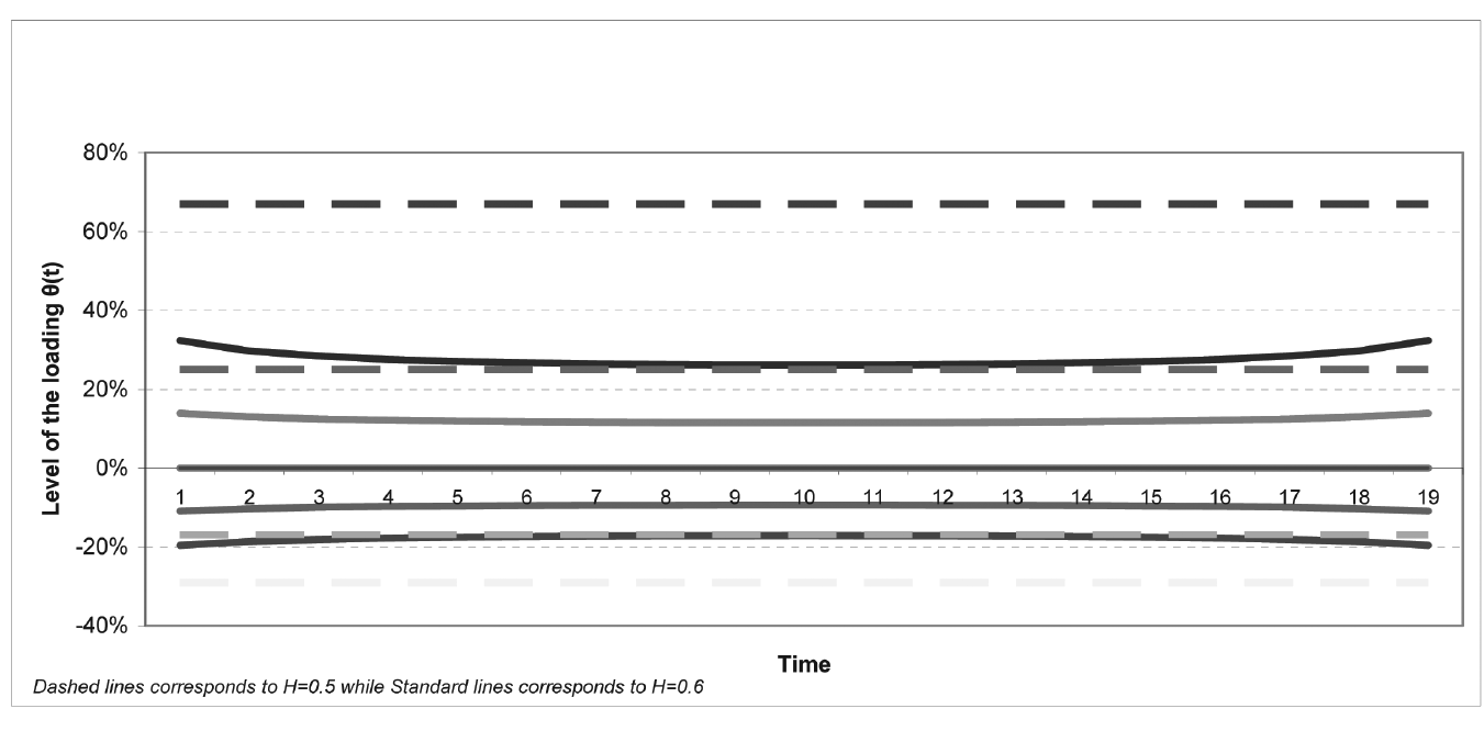
The loading is charged (increasing or decreasing the premium accordingly) to the clients to balance the deficit/surplus of the reserve fund. We simulate the system using two different values for the Hurst exponent. First, we assume H = 0.5, (i.e., there is no long-range dependency within the movements of the market’s average premium rate), while for the second run we assume that H = 0.6 (i.e., as the empirical data suggest there is some kind of long-range dependency within the market). The results are presented in Table 3 and Figure 3. As we observe, the loading is constant for any time t = 1, 2, . . . , 19 when there is no long-range dependency in the market, while the loading is a variable quantity when the long-range dependency truly exists.

Now let us try some intuitive glances on its development.

For solvency ratio 60% and H = 0.6 the value of the safety margin is starting at 32%, considerably lower than 67%, which is the value of the safety margin for the same solvency ratio but for H = 0.5. That is also the case for all the values of H = 0.7, 0.8, 0.9, 1.0. That means the control law overreacts for simple Brownian motion, while it remains more relaxed (as regards the correction of the solvency ratio to unity) for fractional Brownian motion, anticipating some kind of automatic correction due to long-range dependency.

Additionally, we observe a downward movement as t approaches the middle of the control period T, but a return to the initial level with an upward movement as t approaches the end of control period T. That may be interpreted in line with the argument described above, i.e., as time evolves, the control law “feels more relaxed,” anticipating some kind of automatic correction, so it reduces the level of safety margin until the middle of the control period. After passing the middle, the control law becomes more anxious to correct the solvency ratio, so the safety margin returns to its initial values.

7. Conclusions

This paper investigates the insurance pricing process within the context of a competitive market, where the business volume is directly connected to the relationship of the company’s premium and the market’s average premium. The basic contribution is the introduction of fractional Brownian motion as the modeling tool for the driving force of the market’s behavior. The concept of fractional Brownian motion is supported by the empirical evidence found within the data of the Greek motor insurance market for the years 1998–2006.

The final optimal premium strategy described by Equation (20) in Theorem (5.1) and the respective limiting cases in Theorem (5.2) for the different quantities involved appear quite reasonable and intuitive. The premium reduces when the actual fund level exceeds the central value F₀ and approaches the limiting value of zero when the fund value goes to infinity. The opposite result holds when the fund level approaches zero.

Regarding the numerical application, we can identify the fact that the optimal premium control strategy differs considerably from the straight line when there is some kind of long-range dependency H = 0.6, while it remains time invariant when the dependency does not exist H = 0.5.

Finally, we state that there is plenty of room for future research and especially for the solution of this model using other more sophisticated demand functions. Of course, the respective analysis will be much harder as the stochastic optimization tools available for the fractional Brownian motion are quite restricted.