A Review of ML Techniques for Vehicle Symbols Determination

1. Introduction

“Vehicle symbols” (henceforth VS) are codes that group vehicles experiencing similar loss costs. Insurance carriers writing motor peril coverages would typically charge vehicles belonging to the same VS group, the same price — all policyholder characteristics being equal, as described by Verisk (2019). In practice, a vehicle is assigned to a group, typically based on its manufacturer, model, and year, which corresponds to a loss relativity. Loss relativities typically vary by peril: for the same VS, the relativity of the liability coverage is generally different from the theft coverage.

Insurers may use either externally provided VS or they can determine VS by themselves. In the US market, for example, ISO’s VS are well-known for example. Otherwise, an insurer may determine the VS using its internal data and suitable statistical methodologies (on which this paper elaborates), should its own data being credible and consistent enough. Finally, a hybrid approach may be adjusting an externally provided VS structure to the company’s own portfolio experience, both in terms of the VS grouping and relativities.

In general, it is possible to directly insert the variables related to the vehicle’s features directly in the ratemaking predictive models, instead of mediating them by the use of VS. Nevertheless, marketing, operational, or regulatory constraints may require the use of VS when the vehicle characteristics influence the insurance price. E.g., an insurance carrier may not have a sufficiently sized and homogeneous portfolio to independently price the vehicle risk with enough credibility in its model and thus will need supplementary external data. From a technical perspective, VS are codes that indicate the relative risk of loss for each private passenger vehicle for a given model year. They can be considered as a non-technical translation of clustering. Vehicles are defined by a set of characteristics of a different nature. The combination of manufacturer, model, and year represents the vehicle’s unique identifier, whereas the other variables that describe the vehicle’s physical properties would be of mixed nature, either numeric (e.g. engine power or maximum speed) or categorical (e.g. fuel type or chassis). Therefore the models proposed shall handle multivariate mixed data to find vehicles with homogeneous characteristics that ideally share similar loss costs.

Initial research indicates that very little material is available in current actuarial literature and often belongs to commercial vendors, such as the aforementioned Verisk. Our objective is, therefore, to provide a theoretical background and review current uses and implementations. We will also show a worked example presenting how open and easily accessible tools could be used in the VS estimation framework. Several algorithms will be employed and the performance achieved will be evaluated and compared. Such comparisons will focus on the model performance and also the practical issues that a practitioner could encounter.

Recent advances in computer power have paved the way for more sophisticated algorithms that make more extensive use of data in a wide variety of areas, reaching unprecedented levels of performance. Such algorithms are progressively changing how ratemaking is performed. Machine Learning (ML) methods have been proven to be effective in several traditional actuarial tasks (Frees, Meyers, and Derrig 2016). In this context, we aim to provide and show, alongside all the theoretical background needed, how a VS estimation exercise is carried out by exploiting ML methods. In particular, we aim to apply traditional and consolidated algorithms alongside new and innovative techniques. These range from the Principal Component Analysis (PCA) or the K-Means clustering algorithm (MacQueen 1967; Pearson 1901), to the Mixmod clustering algorithm (MacQueen 1967) or the Deep Learning Autoencoders (Goodfellow, Bengio, and Courville 2016).

The analysis will mainly stress the practical application of proposed techniques. Moreover, our research will provide all the data and tools needed to replicate (and potentially enhance) the results presented, adopting open-source software and publicly available datasets. In particular, the Kaggle’s Allstate Claim Prediction Challenge dataset will be used, as it publicly provides vehicles’ features, some policyholders’ variables and normalized loss data. The models’ implementation will be performed by the R and Python frameworks, while the code of the project will be made available through a GitHub repository.

2. Brief literature review

A VS, known in the UK market as Car Insurance Group (CIG), is an identifier of a cluster, that is comprised of vehicles characterized by similar distributions on at least some of their numeric and categorical variables. Both in the US and the UK market, Insurance Bureaus propose VS for key motor insurance perils (e.g. liability, physical auto damage, and theft). In the US market, Verisk (the most important VS provider) publishes VS for Personal Auto Physical Damage (PAPD) and Liability and PIP/Medical Payment (LPMP) auto perils. Verisk uses the vehicle retail price to initially group vehicles for the PAPD peril, while a predictive model based on some vehicle characteristics (e.g. curb weight and chassis type) is used to rank vehicles for the LPMP peril. A similar methodology is used in the Canadian market (Tabachneck and Sattar Al-Khalidi 2006), where a classification system (the Canadian Loss Experience Automobile Rating, CLEAR) is based on a predictive model using many vehicle characteristics as the sole new car price has been shown ineffective. In the UK market, the Association of British Insurers (ABI) uses 50 CIGs, based on a joint work between a Group Rating Panel (from the insurers’ side) and Thatcham Research that provides data on vehicle characteristics (Thatcham Research 2020). In particular, new car price, parts’ pricing, vehicle performance, car security features and level, and the autonomous emergency braking are considered in defining the ABI CIG. VS are recommendations only, as any Insurers can modify vendor-provided rating rankings according to their own loss experience or deriving them without any external input other than their data.

Nevertheless, the literature is very scarce about this topic, as few, if any, publications have been found in scholarly journals explicitly focusing on the classification of vehicles according to their characteristics as they relate to insurance loss cost assessment. Ingenbleek and Lemaire (1988) applied PCA to identify sports cars for ratemaking purposes, whilst Rentzmann and Wuthrich provide a recent review of modern unsupervised learning techniques applied to vehicle data (Rentzmann and Wuthrich 2019). Thus, the existing literature mostly consists of presentations of past actuarial seminars regarding pricing methodologies.

Boison discusses how pricing has been sophisticated during the decades moving from considering just the vehicle age (or year) toward taking into account at least the model (Boison 2011). Guven proposes a framework based on initial multivariate models (on a peril basis) to predict loss cost as a function of vehicle characteristics for a company willing to determine VS using internal-only data (Guven 2009). Guven further proposes to use spatial smoothing methodologies (similar to those employed on territorial ratemaking) to cluster vehicles based on characteristic similarities, but without providing additional details.

P&C actuaries apply clustering and other non-supervised learning techniques not only for VS determination. Two other notable applications of clustering are territorial ratemaking and merging Workers Compensation classes into groups with similar excess ratios. A synthesis of the industry approach on territorial ratemaking is provided by Eliade Micu (Eliade 2012). Territories are grouped into rating areas that are clustered based on the smoothed residual (the relative difference between the actual losses and predicted pure premiums smoothed with the value of neighboring zones). Also, Yao presents a different clustering approach for territorial ratemaking (Yao 2008).

Robertson (2009) describes the approach followed by NCCI to revise the four hazard groups’ classification of worker compensation (WC) classes (types of businesses) in use at that time into a more refined classification system, based on seven groups. Hazard groups are associated with different excess loss factors (ELF) that are used for WC ratemaking. Broadly speaking, a vector of ELFs has been estimated for each class, using also a credibility adjustment criteria. Then, the K-means clustering algorithm is used to group such classes into a finite number of groups. The optimal number of clusters have been selected also by the aid of statistical indices like the Calinski and Harabasz statistic and the Cubic Clustering Criterion (Milligan and Cooper 1985) as well as by business considerations. A vector of seven variables (related to injury severities and pure premiums) were fed into a principal component analysis, and the first dimension scores were used to rank WC classes into different hazard groups.

3. Methodology

The aim of our paper is twofold. First, it will present several ML techniques, mostly unsupervised, that permit either directly merging vehicles into groups (clustering algorithms) or to uncover much fewer latent dimensions (dimensionality reduction algorithms) that summarize their essential characteristics. Secondly, such techniques will be compared in terms of predictive performance and their practical use will be discussed (easiness of implementation, robustness, and communicability to a non-technical audience). An initial descriptive assessment of the relationship between the identified groupings (or hidden dimensions) and the loss cost will be performed for each technique. Eventually, the techniques will be ranked in terms of the predictive performance of the loss cost.

3.1. Dimensionality Reduction Algorithms

The dimensionality reduction techniques provide a synthesis of the original features into fewer ones (called either factors, latent dimension, or archetypes for example), while retaining as much information as possible.

Our application will discuss the following: Principal Component Analysis, t-Distributed Stochastic Neighbor Embedding, Generalized Low-Rank Models and Deep Autoencoders.

3.1.1. Principal Components Analysis

PCA allows summarizing a large dataset with a smaller number of independent linear combinations of the original variables that collectively explain the variability of the original dataset. It is an unsupervised algorithm since it only involves a set of features (X₁, X₂, …, X_n) and no associated outcome Y. The principal component regression is a supervised application of PCA, where the principal components (or a subset of them) are used as features instead of the original variables.

Let X be a dataset with a high number of features, X_i, and the objective is to find a low-dimensional representation of the data that contains as much of the initial data set information as possible.

The PCA finds a small number of dimensions that preserves as much of the original dataset’s variation as possible by computing a linear combination of the initial features. These linear combinations are called Principal Components.

To reduce the dimensionality of the initial dataset, let’s say from i to k, with $k < i$, it is necessary to sort the principal components in decreasing order of importance and retain the top k of them.

In this context, the level of importance is defined as the level of variance that each principal component retains from the initial dataset.

Each component Z_k could, therefore, be defined as:

$$\begin{align} Z_k &= \phi_{1k}X_1 + \phi_{2k}X_2 + \ldots + \phi_{ik}X_i \\ &= (\phi_{1k}, \phi_{2k}, \ldots, \phi_{ik})^T * (X_1, X_2, \ldots, X_i) \\ &= \phi_k * X \end{align}$$

where $Z_k$ denotes the k-th component, $\phi_{ik}$ the variable loading for the i-th original feature and k-th component and $X_i$ the i-th original variable.

Before directly computing the loadings $\phi_{ik}$, the first step is to compute the covariance matrix of the initial features.

The covariance of two variables, i and j is computed as follows:

$$\begin{align} cov(X_i, X_j) &= E[(X_i - \mu_i) (X_j - \mu_j)] \\ &= E[X_i X_j] - \mu_i \mu_j \end{align}$$

where $\mu_i$ is the expected value of the i feature.

In matrix notation, where X is the matrix of observations, the previous expression could be written as:

$$\Sigma = E[(\mathbf{X} - E[\mathbf{X}]) (\mathbf{X} - E[\mathbf{X}])^{T}]$$

Once the matrix $\Sigma$ has been calculated, it is possible to compute its eigenvalues and eigenvectors.^[1]

The computed eigenvalues $\lambda_k$ represent the variance of k-th principal component, whereas the computed eigenvectors represent the variable loadings $\phi_{k}$.

By sorting the eigenvalues $\lambda_k$ (and the corresponding eigenvectors) from the largest to the smallest it is possible to identify which are the components that retain the most variance from the initial set of features.

As a final step, it is possible to multiply the original dataset $X$ by $\Phi$ (the matrix of variable loadings, i.e. the matrix whose columns contain the ordered sequence of eigenvectors) to obtain a new version of $X$, $X^*$.

In this new matrix, each observation is a combination of the original variables, where the weights are determined by the eigenvector.

It is worth noting that, because the eigenvectors in $R$ are independent of one another, each column of $X^*$ is also independent of one another.

3.1.2. t-Distributed Stochastic Neighbor Embedding

t-Distributed Stochastic Neighbor Embedding (t-SNE) is an alternative methodology to PCA for dimensionality reduction, initially introduced by Maaten and Hinton (2008). The key difference between PCA and t-SNE is that t-SNE is strongly non-linear. Also, as briefly detailed in this section, PCA tries to preserve the global similarities or large pairwise distances of the data, while t-SNE is more concerned with preserving local similarities. Furthermore, whereas the PCA returns the full eigenvector decomposition, the t-SNE procedures produces the projection of each point into the lower-dimensional space, whose number of dimensions must be specified in advance, i.e. it is a hyperparameter.

Similarly to the PCA, since the method is based on the concept of geometric distance, it can only handle numerical variables.

As a broad overview, the t-SNE algorithm optimizes a cost function that computes the difference between the similarities of the data points in the high-dimensional space and in the low-dimensional space. The term similarities indicates the Euclidean distances between data points that have been converted into conditional probabilities.

By optimizing such function, the algorithm tries to find the best data points in the low-dimensional space that preserve the similarities observed in the high-dimensional space.

The similarity of the datapoint $x_j$ to the datapoint $x_i$, is the conditional probability that the point $x_j$ would be in the neighborhood centered on $x_i$. It follows that for the points that are very close, the similarity would be relatively high, whereas for points very far apart, it would be relatively small.

Mathematically, the similarity $p_{ij}$ between the points in the high-dimensional space can be expressed as:

$$p_{i|j} = \frac{\text{exp}(-\|x_i-x_j\|^2/2\sigma^2)}{\sum\nolimits_{k\neq i} \text{exp}(-\|x_i-x_k\|^2/2\sigma^2)}$$

The previous expression calculates the distances between the points $x_i$ and $x_j$ and it divides it by the sum of the distances between the point $x_i$ and all the other points. Moreover, it also assumes that the probability densities are distributed according to a Gaussian distribution centered at $x_i$. To make this relationship symmetric, we can further define $p_{ij} = \frac{p_{i|j}+p_{j|i}}{2n}$, where $n$ is the number of data points.

Moreover, it is possible to define the similarity $q_{ij}$ between the points $y_j$ and $y_i$ in the low-dimensional space:

$$q_{ij} = \frac{(1+\|y_i-y_j\|^2)^{-1}}{\sum\nolimits_{k\neq l} (1 + \|y_k-y_l\|^2)^{-1}}$$

This formulation is conceptually equivalent to the previous one with one caveat: it employs a Student t-distribution with a single degree of freedom (Cauchy distribution), rather than a Gaussian distribution.

The Kullback-Leibler divergence measures how different one probability distribution is to a second reference probability distribution.

For discrete probability distributions P and Q, defined on the same probability space $\chi$, the Kullback-Leibler divergence is defined as:

$$KL(P || Q) = \sum_{x \in \chi} P(x) log \frac{P(x)}{Q(x)}$$

If we now consider the similarities of $p_{ij}$ and $q_{ij}$, the previous relationship can be written as:

$$KL(P || Q) = \sum_{i}\sum_{j} p_{ij} log \frac{p_{ij}}{q_{ij}}$$

We can now set the Kullback-Leibler divergence as the cost function that needs to be minimized with respect to $y_i$, the data points in the low-dimensional space. By doing so we will minimize the distance between the similarities $p_{ij}$ and the similarities $q_{ij}$; this means that we will find a set of points $y_i$ in the low-dimensional space that best represents the pairwise distances in the high-dimensional space.

To minimize the chosen cost function, it is possible to use an optimization algorithm such as gradient descent. If we consider the equations for $p_{ij}$ and $q_{ij}$ previously presented, we obtain:

$$\frac{\partial KL(P||Q)}{\partial y_i} = 4\sum_j(p_{ij}-p_{ij})(y_i-y_j)(1+||y_i-y_j||^2)^{-1}$$

By optimizing this function it is possible to find the set of points $y_i$, the low-dimensional representation of the high-dimensional data points $x_i$. As far as model tuning is concerned, the main parameter that defines the dimensionality reduction is the so-called perplexity. This hyperparameter defines the balance between local and global characteristics of the data.

Loosely speaking, the parameter is an indication of how many neighbors each point has. As reported by the original paper: “The performance of SNE is fairly robust to changes in the perplexity, and typical values are between 5 and 50” (Maaten and Hinton 2008).

3.1.3. Generalized Low Rank Models

The Generalized Low Rank Model (GRLMs) is a matrix factorization technique that allows dimension reduction on mixed datasets. It encompasses many well-known algorithms that can be indeed considered special cases of the GLRM family (Udell et al. 2016), for example, the PCA and Singular Value Decomposition (SVD). It is commonly used as a substitute for the PCA, as it naturally handles mixed data sets containing ordinal, categorical, integer, and boolean data types columns; a distinct loss function correspond to each column type. They approximate an input data matrix $X_{m,n}$ by projecting it in a reduced low-rank form, in the k-archetypal space:

$$X_{m,n} \approx A_{m,k}*Y_{k,n}$$

Both $Y_{k,n}$ and $A_{m,k}$ are the outputs of the model; $Y_{k,n}$ constructs the archetypes as a linear combination of original features, while $A_{m,k}$ contains the projection of each $m$ data row in the $k$ archetypal space. As described in the aforementioned literature, $A$ and $Y$ matrices are estimated by numerical alternating minimization algorithms to minimize a loss function that is composed of single columns’ loss functions. Typically, a validation set is provided that is equal to the training one, but a certain percentage of values set randomly as missing. The loss evaluates the discrepancy of the decomposed matrices to reconstruct the original values. GLRMs are defined by the columns’ loss functions (that vary according to the columns’ type) as well as by some hyperparameters that allow regularization in the training process as they encourage sparsity and non-negativity. The optimal configuration of the hyperparameters is found by grid search.

The GLRM framework is quite novel and yet not widely diffused. Apart from missing value reconstruction, another practical application is for products’ recommendation using a collaborative filtering approach (Kallus and Udell 2016), for which an insurance application is presented in Spedicato and Savino (2020).

3.1.4. Autoencoders

The Autoencoders belong to the Neural Networks models family and they are used to learn feature representations in an unsupervised manner. A vanilla autoencoder takes a high dimensional data point as input, its encoding module converts it into a lower-dimensional features part (latent dimension) and then its decoding module tries to reconstruct the original data with just the latent vector with loss of information as minimal as possible. Autoencoders have been used for dimensionality reduction, as they can be considered as a strongly nonlinear generalization of PCA. Variational autoencoders also try to fit a distribution on the latent dimensions; they are used to generate synthetic new data given a (very) large input data set also for actuarial applications (Kuo 2019).

This setting, as it stands, would not be particularly interesting; the network is just learning its input. However, the most useful part of autoencoders is the middle layer, which represents the encoded data.

Since the decoder can reconstruct the input from the middle layer, this layer can be interpreted as a low-dimensional representation of the input data.

Figure 1.Autoencoder

In Figure 1, the input data has been encoded from 10 dimensions to 3 dimensions. In other words, the middle layer is a 3-dimensional representation of the input data.

During the training phase, the model is often penalized so it is forced to learn only some main aspects of the data and not to replicate the training set perfectly. This allows the model to better isolate the signal from the noise and learn useful features of the input data.

This usually happens because the encoded data, i.e. the middle layer, has a smaller dimension than the original data, and so the initial network layers, i.e. the encoder, is forced to retain only the main characteristics of the input data that still permits the final network layer, i.e. the decoder, to reconstruct the initial training data.

On the other hand, if the middle layer is too big, and the network has too much capacity, it may extract non-essential information from the data. As often happens in the field of deep-learning, setting hyperparameters is a very delicate and crucial step.

In the actuarial literature, Autoencoders have been explored for mortality forecasting and telematics (Hainaut 2018; Richman 2018).

3.2. Unsupervised Clustering Algorithms

Clustering indicates the unsupervised process of finding groups in data that share similar characteristics; elements belonging to the same clusters are more similar to each other than to elements belonging to other ones.

Clustering techniques already have several known actuarial applications both in life (Gan and Valdez 2020) and P&C (Yao 2016) areas. The literature traditionally divides the many algorithms into two broad families: partitional and hierarchical. A partitional algorithm aims to divide the dataset into non-overlapping clusters, such that each data point belongs to exactly one cluster. On the other hand, a hierarchical algorithm produces nested clusters that resemble the structure of a tree, called dendogram. Other algorithms, many developed more recently, can be allocated in a third category, the “fuzzy clustering” approached. A fuzzy algorithm does not allocate a point to a single category, instead, it provides an adherence measure (possibly in the form of a probability distribution) of the data point to each cluster.

3.2.1. K-Means

The K-Means algorithm is one of the most popular partitional clustering methods; it aims to partition a set of data points into k clusters, where each observation belongs to the group with the nearest mean. It is an iterative algorithm that finds clusters by minimizing the Euclidean distances between points, hence it minimizes the within-cluster variances. Its computational rapidity and scalability to large datasets significantly contribute to its popularity.

As mentioned, the K-Means algorithm is an iterative algorithm, that can be synthesized as follows:

1. A set of k points, $x_1, x_2, ..., x_n$, are selected to be the centroids of the clusters. Two methods of centroid initialization are the Forgy method and the Random Partition method (Hamerly and Elkan 2002);

2. For each data point, the Euclidean distance between the points and the centroids is computed. Each data point is assigned to the cluster with the closest centroid;

3. Once every point has been assigned to a cluster, the centroids are re-calculated by taking the means of all the points belonging to each cluster. These are the new cluster centroids;

4. The Euclidean distance between the points and the centroids is re-calculated and the points are re-assigned. Steps 2 and 3 are repeated until the centroids do not vary. The final two outputs of the algorithm are the cluster centroid coordinates and the clusters to which each data point belongs.

In the previous description, we assumed that the number of clusters, k, was given in advance. Various approaches have been proposed in the literature to find the optimal number of clusters, a few of which are presented in this section: the Elbow method, the Silhouette method and the Calinski-Harabatz statistic.

The Elbow Method is a graphical approach often used, as relatively fast and easy to implement at the cost of subjectivity. Within the context of the Elbow algorithm, the distortion is defined as the average of the squared distances from the points to the cluster centers of the respective clusters. As k increases, the sum of squared distance tends to zero. If we set k, to its maximum value n (where n is the number of samples) each sample will form its cluster, meaning that the sum of the squared distances equals zero.^[2]

The distortion measure is calculated for each value of k iteratively, starting from 1 to a maximum value of possible clusters. These values are plotted with respect to the value of k so it is possible to visualize and choose the optimal value for the number of clusters. It will be the value of k after which the distortion starts to decrease linearly, i.e. the elbow. The Silhouette Method is based on measuring how similar a point is to its own cluster compared to other clusters. A similarity measure $a(i)$ is defined as the average distance of point $i$ to all the points in the same cluster, while a dissimilarity measure, $b(i)$, is the minimum of the distance between point $i$ and all the other points in other clusters.

The Silhouette value of a clustered point $i$ is then defined as $s(i) = \frac{b(i)-a(i)}{max(a(i),b(i))}$, whose value lies between +1 and -1 by construction. The higher $s\left(i\right)$, the more appropriate the cluster allocation is given to $i$. The mean $s\left(i\right)$, $S$, is the synthetic measure of the proposed clustering solution. The optimal $k$ is the one that maximizes $S$. The Calinski-Harabasz statistic (known also as the Variance Ratio Criterion), is the ratio of the sum of between-clusters dispersion and of inter-cluster dispersion for all clusters. A higher statistic indicates better performance. It has been one of the criteria used to determine the NCCI excess ratio groups in Robertson’s paper (Robertson 2009).

A major drawback of the traditional K-Means approach is that it only uses numerical inputs. Modifications of the original approach, the K-Modes, and K-Prototypes, have been proposed by Huang (1998) to allow the modeling of mixed datasets. The K-Modes algorithm uses a matching dissimilarity measure to deal with categorical objects, replacing the means of clusters with modes, and uses a frequency-based method to update modes in the clustering process to minimize the clustering cost function. One extension of this approach, the K-Prototypes algorithm, further integrates the K-Means and K-Modes algorithms through the definition of a combined dissimilarity measure.

3.2.2. Combined Multivariate Gaussian-Multinomial Mixture Models

In this section, we will look at Combined Multivariate Gaussian-Multinomial Mixture Models (MMM for simplicity) generally used to cluster mixed data sets.

MMM assume that the data points are drawn from a multivariate distribution. This distribution is a finite mixture of multivariate mixed distributions, usually Gaussian and multinomial, each of them representing the data generating process of a specific cluster.

Such models have been explored in actuarial applications in the context of clustering for data compression (O’Hagan and Ferrari 2017) in order to simulate annuity policy behavior.

The analysis presented in the article employs data compression to make simulations of the behavior of the entire portfolio over a large range of stochastic scenarios that are practical to run.

Let the dataset $X = \{x_1, \dots, x_n\}$ be made of $n$ (number of observation in the dataset) independent d-dimensional vectors (d represents the number of features in the dataset), such that each $x_i$, ie, each dataset observation, arises from a mixture probability distribution with density:

$$f(x_i|\theta) = \sum_{k = 1}^{K}p_kh(x_i|\alpha_k),$$

where $p_k$ (K represents the number of clusters, e.g. the number of VS) indicates the proportions ($0 < p_k < 1$, $\sum_{k}{p_k = 1}$), and $h(\cdot| \alpha_k)$ represents a d-dimensional distribution with parameters $\alpha_k$.^[3] The whole parameter vector of f to be estimated is, therefore, $\theta = (p_1, p_2, \dots, p_k, \alpha_1, \alpha_2, \dots, \alpha_k)$.

In order to assign an observation $x$ to a vehicle symbol $k$, we select the value of $k$ that maximizes the probability that $x$ was drawn from $h(x_i|\alpha_k)$. When dealing with labeled data (supervised learning), drawing a sample x from the mixture distribution f, requires first to identify the dataset labels $z = {z_1, \dots, z_n}$. with $z_i = (z_{i1}, \dots, z_{ik})$, $z_{i,k} = 1 \text{ or } 0$, if $x_i$ belongs to the kth component or not.

When, instead, the labels $z_i$ are completely unknown, it is a problem of cluster analysis (unsupervised learning) and there is the need to estimate the clusters $z_i$, $i = 1, \dots, n$, e.g. the likelihood that each observation i belongs to the kth VS.

This can be achieved by implementing the maximum a posterior rule (MAP):

$$\hat{z}(\theta) = \mbox{MAP}(t(\theta)) = \begin{cases} 1, & \mbox{if } k = \mbox{argmax}_{k' \in {1, \dots, K}} \mbox{ }t_{ik'}(\theta) \\ 0, & \mbox{otherwise}\end{cases}$$

where $t(\theta) = {t_{ik}(\theta)}, t_{ik}(\theta)$ indicates the conditional probability that the observation $x_i$ arises from group k:

$$t_{ik}(\theta) = \frac{p_kh(x_i|\alpha_k)}{f(x_i|\theta)}$$

For each observation i we will have a vector of k probabilities that represents how likely it is that the observation i belongs to the class k, i.e. the kth VS.

3.2.3. The OPTICS and DBSCAN algorithms

Many clustering algorithms require the input of a series of parameters to identify the clustering structure, e.g. the number of clusters in the K-Means algorithm. Moreover, the intrinsic cluster structure of many data sets cannot be characterized by global density parameters. This is especially true for hierarchical clustering, where a different set of parameters is needed to identify clusters at each level of the dendrogram.

Density-based approaches overcome this drawback and usually require fewer parameters to identify a cluster, e.g. the DBSCAN (Ester et al. 1996) algorithm only requires two parameters, the radius of a cluster $\varepsilon$ and the minimum number of points in each cluster (MinPts), nevertheless finding the parameters can often be an extremely difficult task.

The OPTICS algorithm (Ankerst et al. 1999) extends the DBSCAN algorithm, only requiring the minPts parameter.

Both the DBSCAN and the OPTICS algorithms have been explored and implemented in the context of actuarial modeling and insurance applications (Diana et al. 2019), such as, for example, in territorial clustering (Yao 2008).

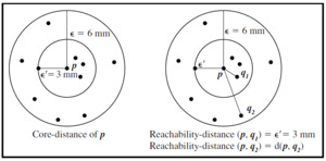
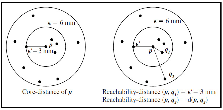
These approaches are based on the concepts of core points and border points. Core points are defined as points inside of the cluster, whereas border points are defined as points on the border of the cluster. Therefore, the core distance is the minimum $\varepsilon$ to make a distinct point a core point, given a finite MinPts parameter. Finally, the reachability distance of an object p with respect to another object q is the smallest distance from q, if q is a core object; it cannot be smaller than the core distance of q.

Figure 2.Optics Terminology, Ankerst et al. (1999)

These definitions are used to create the so-called reachability plot, which will then be used to extract the clusters. It is a plot with the ordering of the points as processed by the OPTICS algorithm on the horizontal axis and the reachability distance on the vertical axis. Since points belonging to a cluster have a low reachability distance to their nearest neighbor (due to being geometrically closer), the clusters show up as valleys in the reachability plot. The deeper the valley, the denser the cluster.

The process starts by calculating the core distances on all data points in the set. Then, by looping through the entire data set, the reachability distances are updated, processing each point only once.

The algorithms only update reachability distances of points that stand to be improved and have not yet been processed. The next data point chosen to be processed will be that which has the closest reachability distance; this is how the algorithm keeps clusters near each other in the output order.

Once the reachability plot has been created, the next step is to extract the actual cluster labels from the plot. The most common way of doing this is by using local minimums and maximums. Each point is assigned to either a cluster or classified as noise.

3.3. Supervised clustering algorithms

3.3.1. Tree-based approaches

Classification and Regression Trees (CART) are among the most important supervised ML algorithms. They can split the dataset into smaller subsets that are recursively defined in terms of intervals of the independent variables. By doing so, CARTs unravel interactions between variables and represent them in terms of hierarchical dependency structures in a form that is also easy to graphically represent and to communicate to a non-technical audience. The C5.0 algorithm is one of the most mature CART implementation (Kuhn et al. 2018). They are often used by actuarial practitioners and in the actuarial literature as can be seen in Derrig and Francis (2006) and Hadidi (2003).

The model-based recursive partitioning approach (MOB) integrates the uses of CART and parametric models (as GLM). In particular, given the partitioning variables, a parametric model is fit. Then, should parameter instability be found using proper statistical testing, the model is split according to the variable associated with the highest instability, and the process is recursively repeated for all sub-samples as fully detailed in Horton and Zeileis’ methodological papers (Hothorn and Zeileis 2015; Zeileis, Hothorn, and Hornik 2008). As of summer 2020, Valdez and Quin provide the only actuarial application of MOB found in the literature (Quan, Gan, and Valdez 2018).

In our application, a simple (constant) GLM on the frequency, with a measure of exposure as the offset, is the parametric model for the leaves, whereas vehicle characteristics variables represent the partitioning ones.

In addition to the well-known advantages in terms of easiness to fit and explainability, as they can represent clusters by recursive splits of input variables, their supervised - learning nature can be considered a clear advantage as identified clusters can be naturally ranked by expected frequency.

This paper applies the CART approach to the identification of VS as it is the only major supervised algorithm, known to the authors, that leads to a finite set of predictions depending on the value of the input features. In fact, each leaf of the tree corresponds to a distinct prediction, and therefore each leaf corresponds to a VS. As it yields to a “supervised” clustering, such prediction can be used as VS.

4. Application

The research will focus on how vehicle characteristics affect insurance risk, keeping them as the primary point of view. This means that each discussed method shall identify groups of vehicles that share similar characteristics, the VS, and shall investigate how VS are related to insurance losses. As discussed in the introduction, predictive modeling approaches that directly use the vehicle variables jointly to non - vehicle ones will not be considered, despite that they may offer sensible results or even better predictive performance for their greater degrees of freedom and the accounting of some shared information between the included ratemaking factors.

Our analysis will present the dataset structure and preparation, then it will briefly discuss each selected ML method separately by providing some graphical representation if deemed appropriate, and reporting one-way analysis of the relationship between insurance risk and either the identified cluster or the latent dimensions identified by the model. The presented plots will be constructed according to the output of the model implemented. If the algorithm returns a continuous score, the plot will be ordered according to the percentiles (deciles) of the score; instead, if the algorithm outputs cluster labels, the plot will not be ordered.

The presented models will therefore be overall compared in terms of predictive performance in the final section. All the results presented are based on the test set portion of the initial full dataset.

The data limitations, detailed in the forthcoming section, made frequency modeling (instead of pure premium) the only viable analysis. Also, only one kind of loss was available for modeling, the third party liability cover.

The R (R Core Team 2020) statistical environment and the Python programming languages (Van Rossum and Drake 2009) were used to implement the practical analysis.

4.1. The dataset

The Kaggle’s competition Allstate Claim Prediction Challenge (Kaggle 2011) is the dataset used for the application of the discussed algorithms. The Allstate competition aimed to “uncover new insights on how vehicle characteristics impact the loss propensity in addition to known effects from other variables domain”.

In the provided dataset, a vehicle is defined by the following variables: model id, model year, categorical covariates (Cat1, Cat2, …, Cat8) and numerical ones (Var1, Var2, …, Var12), all blinded. Each row represents a policyholder for which, in addition to the aforementioned vehicle characteristics, few non - vehicle covariates, as well as exposure and dollar losses, were provided. Before running the analysis, however, the data test has been aggregated at the policyholder-vehicle level.

The original data set contains data for 13 million exposures. In particular, the loss figure provided in the dataset was “adjusted” by controlling for non-vehicle variables affected without disclosing the approach. The appendix shows few descriptive analyses on the provided data set.

Pre-processing has been performed using the R Statistical Software (R Core Team 2020). In particular, the following choices have been selected:

1. considering Model Years before 2009 and excluding observations with any missing in vehicle identification data (Make, Model, Submodel and model-year);

2. exposures, number of claims, and claims amount have been aggregated at vehicle identification variables level;

3. categorical covariates have been aggregated using the mode at the vehicle level.

Policyholders’ data have then been aggregated at vehicle identification level on which all the paper’s analyses have been performed, aggregating the number, the cost, and the exposures at the vehicle identification level, reducing the total size to about 13K records. This final dataset has been further split according to an 80/20 ratio into train and test sets. Each combination of vehicle model and year will therefore appear either in the train or test set, i.e. there will not be duplicate entries across the two sets.

The Allstate competition data set is large enough to permit the application of all the proposed methods. Also, as it is freely available it is easy to independently reproduce and expand our analyses. However, the application part had to face some limitations. First, all vehicle-characteristic variables are blinded, thus it is impossible to identify the meaning of each variable. This makes the models’ interpretation not possible. As a consequence, models have been applied straightly without the use of expert judgment and a deeper analysis of their outcomes. In addition, for sake of simplicity and as the methodology to adjust the claim severity was not disclosed, the insurance risk has been proxied by the frequency only disregarding the severity component (and the pure premium as well). This does not imply that the presented approaches lose generality for being applied to loss costs. Finally, VS were derived for liability peril only, as the sole peril the dataset provided.

4.2. The Principal Component Analysis

The h2o (LeDell et al. 2020) R package has been used to perform the principal component analysis of the dataset. The h2o statistical library is a statistical package that provides high efficient implementations of most common ML algorithms (both supervised and not); it is available both for R and Python.

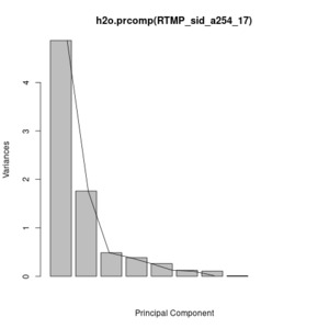
The PCA will be performed on numerical variables only, thus only variables Var1-Var8 were used for this analysis.^[4] The resulting PCA scree plot indicates that the first two principal components explain more than 82% of the numeric variables’ total variability, leaving the residual fraction to the other components.

Figure 3.PCA screeplot

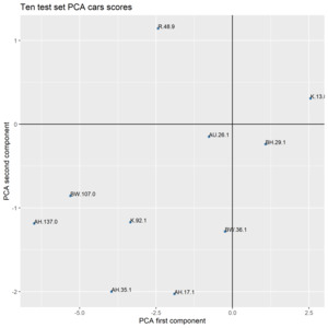
Figure 4 displays ten sampled cars from the test set projected on the two-dimensional space determined by the first two PCA components. This plot, similarly to the other representations that belong to methods based on latent dimensions, may constitute a graphical tool to represent both current and new cars in a metric space.

Figure 4.PCA two dimension projections

To understand whether such principal components are related to loss, as for other methods herewith discussed, PC scores are divided into decile buckets in the test set. For each bucket, the average frequency is calculated.

Figure 5.Principal components vs frequency, one-way analysis

There were no computational issues in applying PCA, thanks to the efficient implementation of the algorithm in the H2O suite and the limited size of the data set.

4.3. The t-SNE algorithm

The t-SNE algorithm has been applied to the initial dataset to perform a dimensionality reduction of the initial feature-space. The initial numerical variables have been projected into a lower 3-dimensional space.

The drawback of this approach, due to the nature of the algorithm itself, is that it is not possible to directly compute the learned mappings on the test set.

To overcome this issue, we decided to train a multi-layer perceptron on the input data, keeping the projected dimensions as targets and then predict the location of the mappings on the test data.

The projected dimensions have been used as the basis to define the clusters of the dataset. Each vector has been divided into deciles and the respective loss experience has been analyzed.

Figure 6 analyzed the relationship between the t-SNE deciles and the claim frequency for each dimension projected by the t-SNE algorithm:

Figure 6.t-SNE Deciles vs frequency, one-way analysis

As it is possible to observe, each lower-dimension representation highlights well-defined and separated clusters that correspond to a different level of claim frequency.

From an implementation standpoint, the t-SNE algorithm could be quite time consuming, also exacerbated by the additional multilayer perceptron needed to make the predictions. Furthermore, the same problem will arise when trying to assign symbols to new vehicles. Overall, when adopting this approach, computational power should be taken into consideration.

4.4. The K-Means clustering algorithm

The h2o suite offers an efficient implementation of the K-Means algorithms in terms of computational performance, also implementing an automatic suggestion of the optimal number of clusters and the capability of handling mixed data.

Our analysis performed two different K-Means runs: the first used only the numerical variables, while the second one also included the categorical variables. The optimal solution, found using a modified Calinski-Harabasz statistic as implemented in the H2O package, identified five clusters with numeric-only variables, while the mixed-data approach identified six. Empirically, it appears an internal consistency between the two approaches as there is a clear strong association between the groups found by the two different approaches (see Table 3).

Therefore, the mixed-variables approach has been used to identify VS with the K-Means method. Figure 7 depicts the relationship between claim frequency and identified clusters.

Figure 7.Mixed data H2O Kmeans

The optimal number of clusters found following a pure statistical framework is six, significantly smaller than the usual figures of typical VS systems. This may lead to a poor predictive performance, and may be a starting point for further investigations.

4.5. The Generalized Low Rank Models

The h2o suite was the natural choice for the GLRM application, as, currently, it is the only available software implementing the algorithm.

The GLRM model was set out using the following assumptions:

1. regularization approach: L1 (ridge);

2. hidden dimension (# or archetypes): chosen over a grid of $(3, 4)$;

3. regularization parameters for $A$ ($\gamma_x$) and $Y$ ($\gamma_y$): chosen over a grid of $(0, 0.1, 0.25, 0.5)^2$.

An initial grid search performed on the train set allowed to identify optimal hyperparameters that were applied to perform the GLRM decomposition on the test set. Then, corresponding archetypal scores were extracted. The overall process was relatively rapid. The best hyperparameters configuration found was: $k=4, \gamma_x=0.5, \gamma_y=0.5$.^[5]

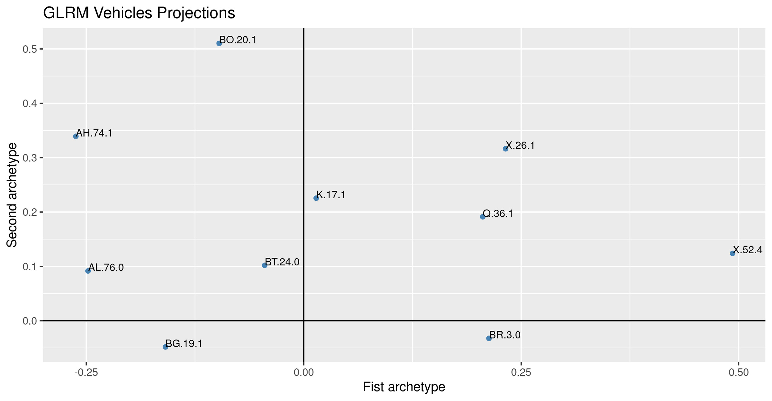
It is possible to represent the vehicles in the reduced archetypal space, as done for PCA (see Figure 8).

Figure 8.GLRM two dimension projections

Figure 9 depicts the relationship between the archetypes deciles and the claim frequency. The first archetype appears related to the insurance risk.

Figure 9.GLRM archetype Decile vs frequency, one-way analysis

4.6. The Mixmod clustering algorithm

The Mixmod package (Lebret et al. 2015) offers a suite of models to cluster multivariate Gaussian (numerical data) or multinomial (categorical data) probability distribution functions to a given dataset. It offers the option to fit up to 28 multivariate Gaussian mixture models for quantitative data and up to 10 multivariate multinomial mixture models for qualitative data using maximum likelihood.

The algorithm works by identifying the data structure, selecting an appropriate model, and computing a target function to evaluate the performance.

Given the data set, which is made of both numerical and categorical variables, we selected composite models based on both the Gaussian structure, for numerical variables, and the Multinomial structure, for categorical variables.

The second step was identifying a suitable number of clusters through a cross-validation approach; several clustering structures were selected and their performances were assessed to identify the optimal number of clusters.

In our analysis, we chose from 2 to 15 clusters and used the Bayesian Information Criterion (BIC) to assess the model metrics: the preferred model is the one with the lowest BIC value.

The clustering rules computed on the train data set have then been applied to the test data set, and Figure 10 shows the relative claim frequency of the assigned clusters.

Figure 10.Mixmod clustering structure

The optimal solution suggested contains 10 cluster, that, however, do not appear all well differentiated in terms of claim frequency.

The procedure could be entirely performed on an average machine without major difficulties. The algorithm is very efficient and well-implemented and it does not require particularly powerful hardware.

4.7. The OPTICS algorithm

The OPTICS algorithm (as its predecessor DBSCAN) only works with numerical data, thus only the variables Var1-Var8 of the data set were used.

The dbscan R package (Hahsler, Piekenbrock, and Doran 2019) has been used to implement the method. It uses a K-Dimensional Tree (K-D Tree) (Hahsler, Piekenbrock, and Doran 2019) which is a binary search tree where the data in each node is a K-Dimensional point in space. The procedure allows the identification of $\epsilon$ and MinPts in an automated way, reducing its complexity.

Furthermore, it allows partitioning the space to organize the points in a K-Dimensional space, where K represents the optimum number of clusters identified.

Figure 11.OPTICS clustering structure

The OPTICS algorithm identifies 7 main clusters with well-separated claim frequencies. The relative frequency of each group appears quite different, despite only numerical variables contributed to the definition of VS groups. The algorithm implemented is relatively fast and efficient. The procedure is very manageable and it does not require advanced systems or hardware.

4.8. Classification and Regression Trees

The R package partykit (Hothorn and Zeileis 2015) has been used to apply Model Based (MOB) Recursive Partitioning on our dataset. As to the authors’ knowledge, that R package is the only viable tool to get (generalized) linear model’s trees. In particular, a naive Poisson regression on the number of claims, using the logarithm of vehicle year as exposure base for offsetting, was used on the final leaves of the partitions identified by the model. All categorical and continuous covariates were used to find the partitions. It is worth to note that the exposure measure may also be the output of a multivariate risk model that uses all ratemaking factors except the vehicle-related ones’.

The minimum number of observations in each leaf has been judgmentally set equal to 250. This is the only hyperparameter that has been altered, and it influences the number of groups identified (it decreases as the minimum size increases).

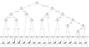
Figure 12 displays the frequency MOB tree on the given dataset.

Figure 12.MOB tree model

It indicates that Cat1, Var3 and Cat3 are the most important variables in explaining frequency differences.

Vehicle groups can be naturally identified using the prediction of the models, that are numerically finite and can also be naturally ranked in terms of loss potential.

Figure 13.MOB groups

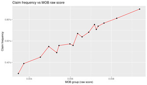
The plot indicates that the MOB model identifies groups from 0.2% to about 0.9% claim frequency and that the predictions are quite stable on a test set.

Computational time are quite fast, but evaluated on a quite small training dataset.

4.9. Autoencoders

The TensorFlow (TF) library (using the Keras front-end) was used to define and fit the autoencoder (AE) model for the scope of this analysis (Abadi et al. 2016; Gulli and Pal 2017). The TF language is probably the most relevant Deep Learning framework as of the second half of 2020 and it permits great modeling flexibility; a suitable alternative, at least for its simplicity, is the H2O suite.

The modeling choices that define the architecture of AE are very wide; the depth of the compression layers, their number of neurons, and the activation functions are just a few of the many options. Moreover, the parameters that drive the estimation process (optimization algorithm, batch size, …) should be taken into account as well.

As the dataset is relatively small in terms of the number of rows and columns, a simple structure has been chosen. An inner four-sized deepfeature layer (bottleneck) and two hidden layers for encoding and decoding define the AE network structure. The tanh activation function and no-dropout showed the best performance given the chosen structure, when comparing different architecture using the reconstruction MSE. More in-depth research would probably lead to a better performing network, but it has not been undertaken beyond the scope of the paper.

As for PCA and GLRM, it is possible to project individual vehicles in a reduced (deep feature or middle layer) space as depicted in Figure 14.

Figure 14.Vehicles representation in Deep Features space

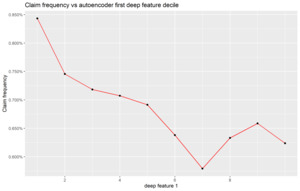
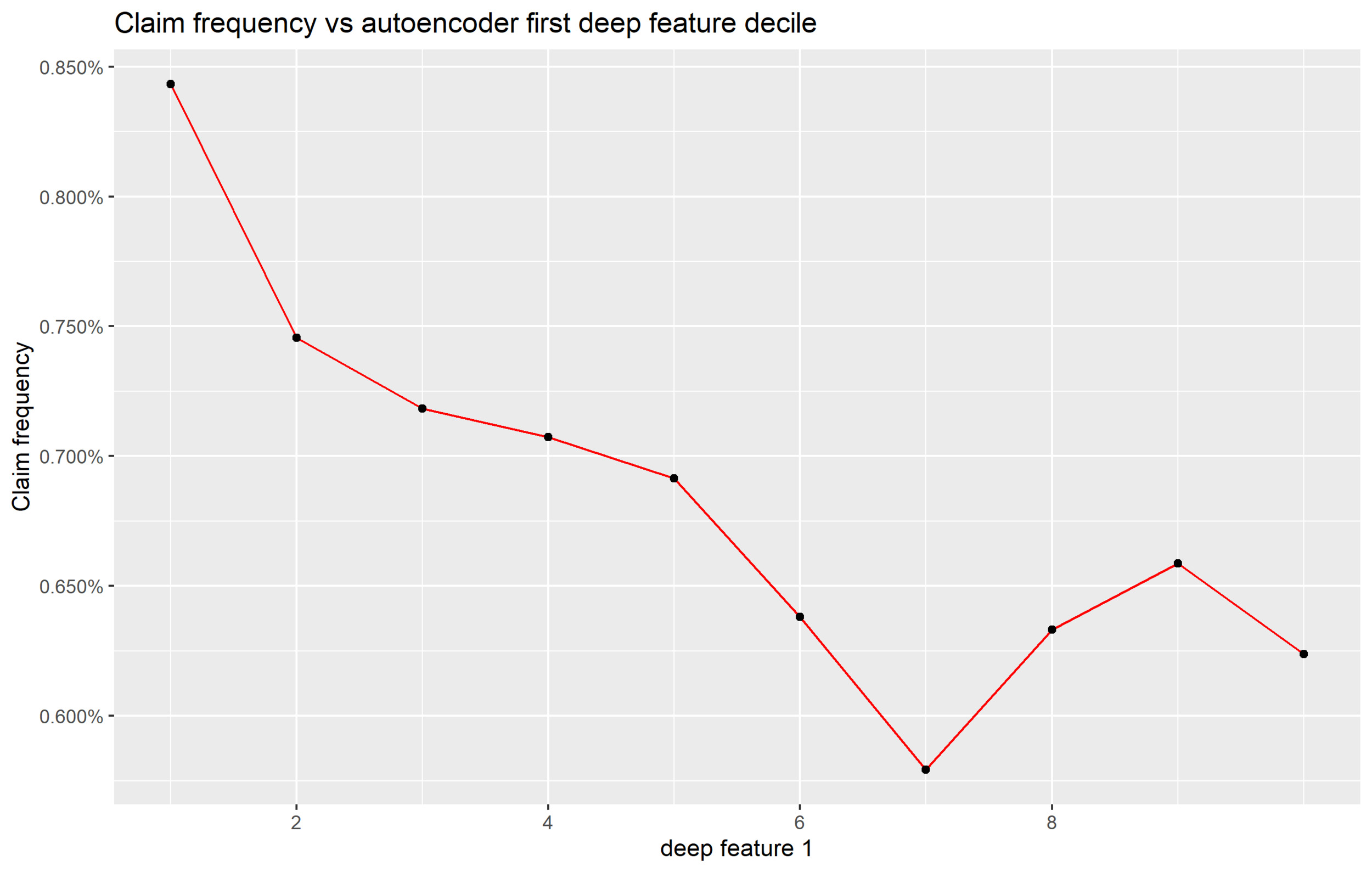
Also, it is possible to assess whether identified deep features have a roughly monotone relationship with the loss potential. Figure 15 depicts the relationship between the claim frequency and the deep feature deciles.

Figure 15.Claim frequency vs deep feature

5. Discussion

5.1. Comparison of methods

The presented ML methods provide as the output either a cluster id (the VS) or latent dimension scores (from which VS can be derived, e.g. binning the given score) as a function of the vehicle features. These obtained VS then become a ratemaking factor to be used in pricing predictive models.

In the context of our analysis, we separately ranked each method according to its ability to predict the claim frequency (as the measure of the insurance risk) using the Normalized Gini Index (Frees, Meyers, and Cummings 2014), which has been used to quantify the methods’ ability to discriminate vehicle propensity to file claims on the test set.

In particular, each ML method has been associated with a univariate model, estimated on the train set, from which a predictive score on a test set has been determined. The predictive score has been based on a Poisson GLM with the target variable being the number of claims for the $i$-th vehicle type ($x_i$), the exposure as an offset, and the method output, $f\left(x_i\right)$, being the independent variable:

$$ln\left(E\left(\lambda_i\right)\right)=f\left(x_i\right)+offset(\ln{\left(Exposure\right)})$$

The $f\left(x_i\right)$ term of the above formula has been defined differently according to the nature of the ML model. When the ML model provides $k$ categorical cluster indexes (so it directly yields to the VS), $f\left(x_i\right)$ is the dummy coefficient of each VS. When the method yields to $k$ latent dimensions ($\eta_i^k$), $f\left( x_i \right)$ is the linear predictor $\beta_k * \eta_i^k$ of the associated GLM. Holding such an approach, we are assessing whether the $k$-th latent dimension shows a monotone relationship with the insurance risk.^[6]

When a cluster index is provided by the ML algorithm, a single model suffices, while one for each latent dimension is computed otherwise.

When the GLMs are scored on the test set, the exposure of each row is set to one. Thus, the GLM scores represent the riskiness of the VS (possibly mediated by the latent dimension) on which the Gini index will be computed.

Table 4 synthesizes the algorithms’ predictive performances.

The CART supervised approach clearly outperforms the other unsupervised methods. However, some latent features of GLRM and Autoencoders show interesting and relatively competitive Gini scores. Additionally, it is interesting to highlight the fact that the CART approach, since supervised, could also be employed to produce different VS for different perils.

It is worth remembering that many of the presented algorithms are themselves defined by a set of hyperparameters and that, in general, the tuning of these algorithms has been limitedly explored. But, while it is possible that the best algorithms’ ranking may be different from the one herewith presented, it is reasonable to suppose that the previous table depicts a reasonable comparison of the predictive power of such approaches in determining automobile liability loss costs.

5.2. Final considerations and aknowledgments

This paper has compared several unsupervised learning algorithms aiming to define groups of vehicles characterized by similar loss propensity, the VS, which is a relevant open issue for the Automobile Insurance business. In particular, well-known algorithms used for decades (as PCA and K-Means) as well as very recently introduced ones (like GLRMs and Autoencoders) have been used for this purpose.

It appears that recent advances in ML techniques may also offer a significant benefit to this aspect of insurance and actuarial modeling. In fact, the predictive power of newer techniques appears to significantly outperform the older ones when compared in terms of Gini score. Also, the GLRM and Autoencoders predictive performances do not appear too far off from the CART result, which is naturally higher for its supervised nature. Many of these algorithms are indeed very new and most likely little known by the predictive modeling practitioners in the insurance sector. This research, therefore, aims to offer an initial introduction to the capabilities of such new techniques, to encourage more in-depth study by actuaries. Moreover, the techniques presented in this article do not imply relevant issues in terms of computational time required (at least due to the typical size of VS datasets), while interpretability may be limited for some.

This paper does not intend to provide a complete review of all the available techniques to perform VS or other similar applications. It is worth to mention that while supervised learning applications are flourishing, as Richman describes (Richman 2021a, 2021b), unsupervised algorithms are much less applied. As the author acknowledges the only two notable applications of unsupervised machine learning are: the DL extension of the Lee-Carter mortality forecasting model (Nigri et al. 2019) and the clustering of driving style habits based on features extracted from DL methods (Wüthrich 2017).

Models’ hyperparameters tuning is just touched on in our analysis. Additionally, other methods not discussed here may also potentially be explored for the stated purpose, i.e. the Multidimensional Scaling (Cox and Cox 2008) or the Multiple Correspondence Analysis (Greenacre and Blasius 2006), just to recall some traditional approaches. The data availability limited the empirical analysis presented only to the frequency of the liability coverage. Nevertheless, the approaches discussed can be applied without any material changes to any auto insurance peril as well as be extended to other contexts.

All the analysis and the code used throughout the paper is public and available at the following GitHub repository: https://github.com/spedygiorgio/CasProject2020VHSymb.

Also a preliminary summary of the paper results has been presented at the yearly CAS Annual meeting, on November 11, 2020: https://www.casact.org/sites/default/files/presentation/cs10-determiningvehiclesymbolsusingmachinelearningtechniques-fileid-261606.pdf. This work has been sponsored by the Casualty Actuarial Society (CAS), the Actuarial Foundation’s research committee, and the Committee on Knowledge Extension Research of the Society of Actuaries (SOA). The authors wish to give a special thanks to all the CAS staff that supported the ongoing research and to the anonymous reviewers who provided extremely useful insights that significantly improved the quality of our paper.

Finally, the opinions expressed in this paper are solely those of the authors. Their employers neither guarantee the accuracy nor reliability of the contents provided herein nor take a position on them.

Appendix

Descriptive analyses

Table 5 shows the summary statistics for all the Numerical (Var) variables.

Code listings

The following code has been included in the GihHub Project Repository:

1. Allstate_claim_load.R: pre-process Kaggle public files to create vehicle-level aggregated data;

2. bivariates.R: one-way analysis

3. h2o_initialize.R initialize functions shared by algorithms using h2o R package;

4. h2o_pca.R script to perform PCA in h2o R package;

5. clustering_h2o_model.R script to perform KMEANS models in h2o R package;

6. clustering_mixmod.R script to perform mixture modeling in RMixmod R package;

7. clustering_optics.R script to perform OPTICS in dbscan R package;

8. predictive_performance_assessment.R: it compares the predictive power of the different methods tested.