Simulation Methods for Compound Distributions

undefined

1. Introduction

In collective risk theory, the total amount of losses an insurance company incurs during a time period is modeled by a compound random variable

\[ S=\sum\limits_{i=1}^M X_i, \tag{1.1} \]

where \(M\) is a discrete random variable representing the number of claims; \(X_1, X_2, \dots\) are nonnegative independent and identically distributed (i.i.d.) claim size random variables independent of \(M\). The tail probability,

\[\theta= \mathbf{P}[S>c]\]

for some specified value \(c\) and the tail mean (mean excess loss), defined by

\[\tau= \mathbf{E}[(S-c)_+],\]

where

\[(S-c)_+=\left\{\begin{array}{cc} 0 & S\le c \\ S-c & S>c \end{array}\right.\]

are important risk measures of \(S\) because they are closely related to insurance/reinsurance pricing and capital requirement.

Evaluation of the tail probability and the tail mean is not easy, even when the distribution of \(M\) and \(X_i\) are known. One approach is to resort to recursive formulas, such as those proposed by Panjer (1981), for the case when the distribution of \(M\) belongs to the \((a,b,0)\) class. There is extensive literature on further developments related to Panjer’s recursive formula. For details, see the comprehensive book by Sundt and Vernic (2009).

Transform-based techniques, such as fast Fourier transform (FFT), are also widely used in calculating the distribution of aggregated claims. For an introduction, see the papers by Robertson (1992) and Wang (1998) and the references therein. Embrechts and Frei (2008) provided an excellent comparison of the recursive and FFT methods.

Simulation methods are flexible and can be handy in estimation of the tail probability/moments of compound distributions. However, they are subject to sampling errors. That is, different runs of the same simulation method will give different results.

For example, the one-sample crude estimator for \(\theta=\mathbf{P}[S>c]\) is

\[ \hat{\theta}_0 = \mathbb{I}(S>c),\]

where \(\mathbb{I}(\cdot)\) is an indicator function that takes the value of one if the argument is true and zero otherwise. \(\hat{\theta}_0\) is an unbiased estimator of \(\theta\) because

\[\mathbf{E}[\hat{\theta}_0]=\theta.\]

The variance of \(\hat{\theta}_0\) is

\[\mathbf{Var}[\hat{\theta}_0]=\theta(1-\theta),\]

and the coefficient of variation (CoV) is

\[ \text{CoV}(\hat{\theta}_0)= \frac{\sqrt{\theta(1-\theta)}}{\theta}=\sqrt{\frac{(1-\theta)}{\theta}}.\]

Quite often, we are interested in a tail probability of \(S\) so that \(\theta\) is close to zero. Then the coefficient of variation \(\text{CoV}(\hat{\theta}_0)\) is huge, which makes the crude method inefficient. Notice that when the simulation is conducted \(n\) times, the estimator for \(\theta\) is

\[ \hat{\theta}_{0,n}=\frac{1}{n} \sum_{j=1}^{n} \mathbb{I}(S^{(j)} >c), \tag{1.2}\]

which has variance \(\frac{1}{n}\theta(1-\theta)\) and CoV

\[ \small{ \begin{aligned} \operatorname{CoV}\left(\hat{\theta}_{0, n}\right) & =\frac{\sqrt{\theta(1-\theta) / n}}{\theta}=\frac{1}{\sqrt{n}} \cdot \sqrt{\frac{(1-\theta)}{\theta}} \\ & \simeq \frac{1}{\sqrt{n \hat{\theta}_{0, n}}}=\left(\sum_{j=1}^n \mathbb{I}\left(S^{(j)}>c\right)\right)^{-1 / 2} . \end{aligned} \tag{1.3} } \]

When \(n\) is large, the distribution of \(\hat{\theta}_{0,n}\) is approximately normal by the central limit theorem, based on which the \(1-\alpha\) confidence interval of \(\theta\) is given by

\[\begin{aligned} \left(\hat{\theta}_{0,n}- {z_{1-\alpha/2}} \sqrt{\mathbf{Var}[\hat{\theta}_{0,n}]}, \quad \hat{\theta}_{0,n}+ {z_{1-\alpha/2}} \sqrt{\mathbf{Var}[\hat{\theta}_{0,n}]}\right). \end{aligned}\]

In other words,

\[ \mathbf{P}\left(\frac{|\hat{\theta}_{0,n}-\theta|}{\theta}\le z_{1-\alpha/2} \text{CoV}(\hat{\theta}_{0,n})\right) = 1-\alpha.\]

Taking \(\alpha=0.1\), this means that with \(90\%\) probability, the relative error of \(\hat{\theta}_{0,n}\), \(\frac{|\hat{\theta}_{0,n}-\theta|}{\theta}\) is less than \(1.65 \text{CoV}(\hat{\theta}_{0,n})\). Therefore, \(\text{CoV}(\hat{\theta}_{0,n})\) can be a measure for relative error.

In fact, for any estimator \(\hat{\theta}\) of some parameter \(\theta\), similar reasoning applies. As a result, \(\text{CoV}(\hat{\theta})\) is a measure of relative error for \(\hat{\theta}\). Therefore, we say that an estimator (simulation method) with a smaller CoV is more efficient.

For our case, the relative error of \(\hat{\theta}_{0,n}\) is given in equation (1.3). When \(\theta\) is close to zero, \(\mathbb{I}(S^{(j)}>c)\) rarely equals one. So \(\sum_{j=1}^n \mathbb{I}(S^{(j)}>c)\) is small, resulting in a large CoV. For example, suppose that the value of \(c\) is such that the tail probability is roughly (from prior knowledge) \(1\%\). If \(n=1000\), we expect that \(\sum_{j=1}^n \mathbb{I}(S^{(j)}>c)\) is around \(10\). Consequently, \(\text{CoV}(\hat{\theta}_{0,1000})\) is approximately \(10^{-1/2} \simeq 0.32\). This means that with a probability of \(90\%\), the relative error of \(\hat{\theta}_{0,1000}\) is within \(1.65\times 0.32= 53\%\), which is not very satisfactory. Increasing the sample size to \(10^4\), the relative error of \(\hat{\theta}_{0,10^4}\) is \(1.65\times 0.1= 16.5\%\), which is still not very accurate. Recalling that \(\mathbf{Var} (\hat{\theta}_{0,n}) = \frac{1}{n} \mathbf{Var} (\hat{\theta}_{0})\), we see that in order to decrease the relative error (CoV) of an estimator tenfold, the sample size has to increase a hundredfold.

Remark 1.1. This discussion may remind actuaries of the situation in limited fluctuation credibility theory, in which the sample size of loss data is determined such that the sample mean will provide a credible (low relative error) estimate of the population mean. The idea there is similar and the same square rule applies. In limited fluctuation credibility, to double the credibility factor, the sample size has to be quadrupled.

In this paper, we study simulation methods (estimators) of the tail probability (\(\theta\)) of compound random variables. As shown, increasing the sample size of the crude estimator is one way to reduce relative error. However, because of the square rule, it is costly and inefficient and sometimes not feasible. Therefore, instead of increasing the sample size, we propose several more efficient estimators of \(\theta\) that, given the same sample size, are still unbiased, yet have a lower CoV (relative error).

Reducing the CoV requires reducing the variance of the estimator. In the simulation literature, various variance reduction methods exist. Commonly used techniques include importance sampling, stratified sampling, the conditioning method, and the control variates method, which we review briefly in the next section. For detailed introductions to variance reduction methods, see, for example, the books by Ross (2012) and Asmussen and Glynn (2007).

Needless to say, simulation methods for evaluating the tail probability and tail mean of compound variables are very important for actuaries. However, quite surprisingly, to our knowledge, the literature in this area is very thin. In addition to some examples from Ross (2012), one of the most relevant references is Peköz and Ross (2004), in which the conditioning method was introduced specifically for compound variables. Blanchet and Li (2011) introduced an efficient importance sampling algorithm for estimating the tail distribution of heavy-tailed compound sums. Glasserman, Heidelberger, and Shahabuddin (2000) proposed a method for simulating tail probability (value at risk) of the returns of investment portfolios by combining the importance sampling and stratified sampling methods.

In this paper, we first briefly review some commonly used general variance reduction methods for simulation, then we propose several novel combinations of variance reduction methods specifically for compound distributions. This includes the combination of importance sampling and the conditioning method and the combination of importance sampling and stratified sampling.

Secondly, we extend our methods to simulate the tail probability and tail mean of bivariate compound variables, defined by

\[ (S_1,S_2)=\bigg(\sum_{i=1}^M X_i, \sum_{j=1}^N Y_j\bigg), \tag{1.4}\]

where \((M,N)\) is a vector of (dependent) random variables representing the number of the claims in two lines of business. The claim size random variables \(X_i\) and \(Y_j\) for \(i, j = 1,2,\dots\) are mutually independent and are independent of the claim numbers \(M\) and \(N\).

The remaining parts of the paper are organized as follows. Section 2 reviews commonly used variance reduction methods. Section 3 applies them in estimation of tail probability. Section 4 studies the simulation methods for the tail mean. Sections 5 and 6 extend the results to bivariate compound variables. Section 7 concludes.

2. Review of variance reduction methods

We start by briefly reviewing several variance reduction methods that will be used in this paper. For more comprehensive introductions to the topic, see books such as those by Ross (2012) and Asmussen and Glynn (2007).

2.1. Importance sampling

Let \(\mathbf{Z}=(Z_1,\dots,Z_n)\) denote a vector of random variables having a joint density function \(f(\mathbf{z})=f(z_1,\dots,z_n)\) and suppose that we want to estimate

\[ \theta=\mathbf{E}[g(\mathbf{Z})]=\int g(\mathbf{z})f(\mathbf{z})d\mathbf{z},\]

where the integral is \(n\)-dimensional and over the support of \(\mathbf{Z}\).

Importance sampling finds the probability density function (PDF) \(f^*(\mathbf{z})\) such that \(f(\mathbf{z})=0\) whenever \(f^*(\mathbf{z})=0\). Since

\[ \theta=\int \frac{g(\mathbf{z})f(\mathbf{z})}{f^*(\mathbf{z})}f^*(\mathbf{z})d\mathbf{z}=\mathbf{E}\bigg[\frac{g(\mathbf{Z}^*)f(\mathbf{Z}^*)}{f^*(\mathbf{Z}^*)}\bigg],\]

where \(\mathbf{Z}^*\) has density \(f^*(\mathbf{z})\),

\[\hat{\theta}_I= \frac{g(\mathbf{Z}^*)f(\mathbf{Z}^*)}{f^*(\mathbf{Z}^*)}\]

is an unbiased estimator for \(\theta\).

The importance sampling approach aims to choose an appropriate \(f^*(\mathbf{z})\) so that \(\hat{\theta}_I\) has a smaller variance compared with the crude estimator \(\hat{\theta}_0= g(\mathbf{Z})\).

Since

\[\begin{aligned} \mathbf{Var}\bigg[\frac{g(\mathbf{Z}^*)f(\mathbf{Z}^*)}{f^*(\mathbf{Z}^*)}\bigg]&=\mathbf{E}\bigg[\bigg(\frac{g(\mathbf{Z}^*)f(\mathbf{Z}^*)}{f^*(\mathbf{Z}^*)}-\theta \bigg)^2\bigg] \notag\\ &= \int \frac{(g(\mathbf{z})f(\mathbf{z})-\theta f^*(\mathbf{z}))^2}{ f^*(\mathbf{z})} d\mathbf{z}, \end{aligned}\]

in order to achieve a smaller variance, \(f^*(\mathbf{z})\) should be chosen such that the numerator \(g(\mathbf{z})f(\mathbf{z})-\theta f^*(\mathbf{z})\) is close to zero. That is, \(f^*(\mathbf{z})\) is proportional to \(g(\mathbf{z})f(\mathbf{z})\).

If \(\mathbf{Z}\) has a finite moment generating function (MGF)

\[M_{\mathbf{Z}}(\mathbf{t})= \mathbf{E}[e^{\mathbf{Z}\cdot \mathbf{t}}]=\mathbf{E}[e^{Z_1t_1+ \cdots+Z_nt_n}],\]

for some \(0<\mathbf{t}<\mathbf{b}\), then it is usually handy to choose \(\mathbf{Z}^*\) to be the Esscher transform (exponential tilting) of \(\mathbf{Z}\). That is, we let \(\mathbf{Z}^*\) have PDF

\[ f^*(\mathbf{z})=\frac{e^{\mathbf{h}\cdot \mathbf{z}}f(\mathbf{z})}{M_{\mathbf{Z} }(\mathbf{h})}\]

for some tilting parameter \(\mathbf{h} \le \mathbf{b}\). In addition, the MGF of \(\mathbf{Z}^*\) is given by

\[M_{\mathbf{Z}^*}(\mathbf{t})=\mathbf{E}[e^{\mathbf{t} \cdot \mathbf{Z}^*}]=\frac{\mathbf{E}[e^{(\mathbf{t}+\mathbf{h})\cdot \mathbf{Z}}]} {\mathbf{E}[e^{\mathbf{h}\cdot \mathbf{Z}}]} = \frac{M_{\mathbf{Z}}(\mathbf{t}+\mathbf{h})}{M_{\mathbf{Z}}(\mathbf{h})}.\]

Notice that if \(\mathbf{Z}\) is a discrete random variable, we interpret \(f\) and \(f^*\) as probability mass functions (PMFs).

For presentation simplicity, in the sequel, we assume that the goal is to estimate the mean of some random variable \(Z\),

\[\theta=\mathbf{E}[Z],\]

instead of \(\mathbf{E}[g(Z)]\) for some function \(g\). Doing so does not lead to loss of generality because \(Z\) can have any form, such as \(Z=g({Z}')\).

2.2. The conditioning method

Suppose that \(W\) is a random variable that is correlated with \(Z\) and can be simulated efficiently and that \(\mathbf{E}[Z\mid W]\) can be evaluated. Then

\[\hat{\theta}_{CD}=\mathbf{E}[Z\mid W]\]

is a more efficient estimator of \(\theta\) than the crude estimator \(\hat{\theta}_0=Z\) because it is unbiased; that is,

\[\mathbf{E}[\hat{\theta}_{CD}]=\mathbf{E}\big[\mathbf{E}[Z\mid W]\big]=\mathbf{E}[Z],\]

and it has a smaller variance, as shown in the following line.

\[ \begin{align} \mathbf{Var}[Z]&=\mathbf{Var}\big[\mathbf{E}[Z\mid W]\big]\\ &\quad +\mathbf{E}\big[\mathbf{Var}[Z\mid W]\big] \ge \mathbf{Var}\big[\mathbf{E}[Z\mid W]\big]. \end{align}\]

2.3. Stratified sampling

Stratified sampling resembles the conditioning method in the sense that a random variable \(W\) can help simulate the mean of a random variable \(Z\). Suppose that \(W\) takes values in \(k\) strata \(\mathcal{W}_1,\dots,\mathcal{W}_k\) with probability \(p_i=\mathbf{P}[W\in \mathcal{W}_i]\) for \(i=1,\dots, k\). Then

\[\mathbf{E}[Z]=\sum_{i=1}^k \mathbf{E}[Z\mid W\in \mathcal{W}_i]p_i.\]

Suppose that \(n\) is the total number of samples and \(n_i\) is the number of samples from stratum \(i\). Then the stratified estimate of \(\mathbf{E}[Z]\) is

\[\hat{\theta}_{S,n}=\sum_{i=1}^k \bar{Z}_i p_i,\]

where for \(i=1,\dots, k\), \(\bar{Z}_i\) is the sample average of \(Z\)s conditional on \(W\in \mathcal{W}_i\).

Let \(\sigma_i=\mathbf{Var}\big[Z\mid W\in \mathcal{W}_i]\), then the variance of \(\hat{\theta}_{S,n}\) is

\[\mathbf{Var}[\hat{\theta}_{S,n}]=\sum_{i=1}^k p_i^2 \frac{\sigma_i^2}{n_i}.\]

If we choose \(n_i= np_i\), then \(\hat{\theta}_{S,n}\) must have a smaller variance than the crude simulation estimator \(\hat{\theta}_{0,n}=\sum Z_i/n\) because

\[ \begin{align} \mathbf{Var}[\hat{\theta}_{S,n}]&=\frac{1}{n}\sum_{i=1}^k p_i\sigma_i^2\\ &=\frac{1}{n}\mathbf{E}\big[\mathbf{Var}[Z\mid W]\big] \le \frac{1}{n} \mathbf{Var}[Z]\\ &= \mathbf{Var}[\hat{\theta}_{0,n}]. \end{align}\]

It is worthwhile to note that \(n_i= np_i\) is not necessarily the optimal number of simulations in stratum \(i\). Particularly, if \(n_i\) is chosen to be proportional to \(p_i\sigma_i\) (Fishman 1995), then \(\mathbf{Var}[\hat{\theta}_{S,n}]\) is minimized.

2.4. The control variates method

When using a control variable to reduce the variance of the estimator of \(\theta=\mathbf{E}[Z]\), we select a control variate \(W\) that is strongly positively or negatively correlated with \(Z\). Then an unbiased estimator for \(\theta\) is

\[\hat{\theta}_{CV}=Z-\gamma (W-\mathbf{E}[W])\]

for some constant \(\gamma\). Then we have

\[ \mathbf{Var}[\hat{\theta}_{CV}]= \mathbf{Var}[Z]+\gamma^2\mathbf{Var}[W]-2\gamma\mathbf{Cov}(Z,W),\]

which is minimized if \(\gamma=\mathbf{Cov}(Z,W)/\mathbf{Var}[W]\). Note that the parameter \(\gamma\) can be estimated using the simulated values of \(Z\) and \(W\). In fact, it is the least square estimate of the slope of the simple linear regression

\[Z=\gamma_0+\gamma_1 W+\epsilon.\]

Obviously, there are many other general-purpose simulation variance reduction methods in the literature. We have only introduced the four that we use for simulating the compound random variables in this paper. In the following sections, we illustrate how these methods can be used in combination to reduce the simulation variance even further.

3. Simulating tail probability

In this section, we apply the four variance reduction methods to the estimation of the tail probability \(\theta=\mathbf{P}[S>c]\), where the compound random variable \(S\) is defined in (1.1).

The one-sample crude estimator is simply \(\hat{\theta}_{0} = \mathbb{I}(S >c)\). The \(n\)-sample estimator is given by \(\hat{\theta}_{0,n}\), defined in (1.2).

The problem with the crude method is that when \(c\) is large, the sample size needs to be very large in order for \(S>c\) to occur. Therefore, as shown in equation (1.3), the crude estimator is not efficient.

3.1. Importance sampling

Let \(f_S(x)\) be the PDF of \(S\).^[1] We assume that \(S\) has finite MGF \(M_S(t)=\mathbf{E}[e^{tS}]\) on the interval \(t\in[0, b)\), where \(b>0\).

In importance sampling, instead of sampling \(\mathbb{I}(S>c)\), we sample \(\mathbb{I}(S^*>c) \frac{f(S^*)}{f^*(S^*)}\), where \(S^*\) has PDF \(f^*\). Since we assume that \(S\) has a finite MGF, we may choose \(S^*\) to be the Esscher transform (exponential tilted transform) of \(S\). That is, we let \(S^*\) have PDF

\[ f^*(x)=\frac{e^{hx} f(x)}{M_S(h)},\]

for some tilting parameter \(h \in (0,b)\). Then we have \[\theta=\mathbf{E}[\mathbb{I}(S>c)]=\mathbf{E}\bigg[\mathbb{I}(S^*>c)\frac{M_S(h)}{e^{hS^*}}\bigg].\]

Hence, the importance sampling estimator of \(\theta\) is given by

\[ \hat{\theta}_I= \mathbb{I}(S^*>c){M_S(h)}{ \exp({-hS^*})}. \tag{3.1}\]

If the sample size is \(n\), then we have

\[ \hat{\theta}_{I,n}= \frac{M_S(h)}{n} \sum_{j=1}^{n}\mathbb{I}(S^{*(j)}>c) { \exp\left({-h S^{*(j)}}\right)},\] where \(S^{*(j)}\) is the \(j\)th simulated value of \(S^{*}\).

In order to apply the importance sampling method with exponential tilting, we need to (1) select an appropriate value for the tilting parameter \(h\), and (2) simulate \(S^*\) with the tilted distribution.

As mentioned in Section 1, the problem with the crude simulation method is that when \(\theta\) is small, \(\mathbb{I}(S>c)\) is zero for most rounds of simulation, which results in a large value of the CoV of \(\hat{\theta}_{0,n}\). In importance sampling, we choose \(h\) such that \((S^*>c)\) is more likely to occur than \((S>c)\). An intuitively natural choice for the value of \(h\) is \(\mathbf{E}[S^*]=c\). This choice is indeed optimal, as the following note shows.

Note 3.1. As pointed out by Ross (2012),

\[\hat{\theta}_I = \mathbb{I}(S^*>c)M_S(h)e^{-hS^*}\leq M_S(h)e^{-hc}.\]

Thus, one can stabilize the results of every round of simulation by choosing the value of \(h\) to minimize the upper bound \(M_S(h)e^{-hc}\). Setting the derivative of it to zero, we get

\[M_S'(h)-cM_S(h)=0.\]

Thus, the optimal \(h\) should satisfy

\[c=\frac{M_S'(h)}{M_S(h)}=\mathbf{E}\bigg[ \frac{S e^{hS}}{M_S(h)}\bigg]=\mathbf{E}[S^*].\]

We next study the distribution of \(S^*\) (in order to simulate it). The result is stated in the following note.

Note 3.2 The Esscher transform of \(S=\sum_{i=1}^M X_i\) with parameter \(h\) is

\[S^* = \sum_{i=1}^{M^*} X_i^*,\]

where \(X_i^*\) is the Esscher transform of \(X_i\) with parameter \(h\) and \(M^*\) is the Esscher transform of \(M\) with parameter \(c(h)= \ln (M_X(h))\).

Proof. Firstly, the MGF of \(S^*\) is

\[ \begin{align} M_{S^*}(t)&=\frac{M_S(t+h)}{M_S(h)}=\frac{P_M(M_X(t+h))}{P_M(M_X(h))}\\ &=\frac{P_M(M_X(h)M_{X^*}(t))}{P_M(M_X(h))}, \end{align} \tag{3.2}\]

where \(P_M(z)=\mathbf{E}[z^M]\) represents the probability generating function (PGF) of \(M\) and \(X^*\) is the Esscher transform of \(X\) with parameter \(h\).

Let \(c(h)=\ln (M_X(h))\) and let \(M^*\) be the Esscher transform of \(M\) with parameter \(c(h)\). Then the PGF of \(M^*\) is

\[ \begin{align} P_{M^*}(z)&=\frac{\mathbf{E}[e^{{c(h)}M}\cdot z^M]}{\mathbf{E}[e^{{c(h)}M}]}=\frac{P_M(e^{c(h)}\cdot z)}{P_M(e^{c(h)})}\\ &=\frac{P_M(M_X(h)z)}{P_M(M_X(h))}. \end{align} \tag{3.3}\]

Comparing (3.2) and (3.3) leads to

\[M_{S^*}(t)=P_{M^*}(M_{X^*}(t)),\]

which shows that \(S^* = \sum_{i=1}^{M^*} X_i^*\). ◻

Note 3.2 suggests that \(S^*\) is a compound sum of \(M^*\) and \(X^*\). Therefore, it can be easily simulated if the distribution of latter two are known. This is actually the case for many commonly used distributions; the following are Esscher transforms (with parameter \(h\)) of some commonly used distributions.

• If \(M\sim \textrm{binomial}(n,p)\) with the PMF \[p_M(k)={n\choose k}p^k(1-p)^{n-k},\quad k=0,1,2,\dots, n,\] then \(M^*\sim \textrm{binomial}(n,\frac{pe^h}{1-p+pe^h})\).

• If \(M\sim \textrm{negative binomial}(r,p)\) with the PMF \[p_M(k)={k+r-1\choose k} (1-p)^r p^k,\quad k=0,1,2,\dots,\] then \(M^*\sim \textrm{negative binomial}(r,pe^h)\), \(h< -\ln p\).

• If \(M\sim \textrm{Poisson}(\lambda)\) with the PMF \[p_M(k)=\frac{\lambda^k}{k!}e^{-\lambda}, \quad k=0,1,2,\dots,\] then \(M^*\sim \textrm{Poisson}(\lambda e^h)\).

• If \(X \sim \textrm{gamma}(\alpha,\beta)\) with the PDF \[f_X(x)=\beta^\alpha x^{\alpha-1}e^{-\beta x}/\Gamma(\alpha),\quad x>0 ,\] then \(X^* \sim \textrm{gamma}(\alpha,\beta-h)\), \(h<\beta\).

Example 3.1. Assume that \(M\sim \textrm{Poisson}(\lambda)\) and \(X_i, i=1,2,\dots\) have common distribution \(X \sim \textrm{gamma}(\alpha,\beta)\). Then

\[S^*=\sum\limits_{i=1}^{M^*}X_i^*,\]

where \(M^*\sim \textrm{Poisson}\left(\lambda (\frac{\beta}{\beta-h})^\alpha \right)\) and \(X_i^*\sim \textrm{gamma}(\alpha, \beta-h)\).

3.2. Combining importance sampling and stratified sampling

A method for applying stratified sampling in simulating quantities related to compound distribution was introduced by Ross (2012, Section 9.5.3). This is done by treating the claim number \(M\) as a stratifying variable. Specifically, in order to simulate

\[\theta=\mathbf{E}[g_M(X_1, \dots, X_M)],\]

we choose a number \(m\) such that \(\mathbf{P}(M>m)\) is small and make use of the fact that

\[ \begin{align} \theta&= \sum_{n=0}^{m} \mathbf{E}[g_{n}(X_1, \dots, X_{n})]p_n\\ &\quad + \mathbf{E}[g_M(X_1, \dots, X_M)|M>m]\left(1-\sum_{n=0}^{m}p_m\right). \end{align}\]

This method can be applied to estimate the tail probability \(\theta=\mathbf{P}[S>c]\) if we let, for \(m\ge 1\),

\[g_m(X_1, \dots, X_m)= \mathbb{I}(X_1 + \cdots+ X_m>c).\]

However, directly applying the method is not efficient because when \(c\) is large and \(\theta\) is small, the function \(\mathbb{I}(X_1 + \cdots+ X_m>c)\) is likely to be zero on most strata, and more so with small values of \(m\).

Therefore, we propose here a method to combine importance sampling and stratified sampling. For this purpose, we let \(S^*=\sum_{i=1}^{M^*}X_i^*\) be the Esscher transform of \(S\) with parameter \(h\) and \(\mathbf{E}[S^*] = c.\)

Define

\[ \scriptsize{ g_m^*(x_1,\dots,x_m)= {M_S(h) \mathbb{I}\left(\sum_{i=1}^m x_i >c\right)} {\exp \left({-h\sum_{i=1}^m x_i}\right)}\tag{3.4}}\]

and

\[p_m^*=\mathbf{P}[M^*=m], \quad m=1,2,\dots.\]

Then we have, for a given value of \(m_l\) such that \(\mathbf{P}[M^*>m_l]\) is small,

\[ \small{ \begin{aligned} \theta &=\mathbf{E}[\mathbb{I}(S>c)]\notag\\ &=\mathbf{E}\bigg[\mathbb{I}(S^*>c)\frac{M_S(h)}{e^{hS^*}}\bigg]\notag\\ &=\mathbf{E}[g^*_{M^*}(X_1^*, \dots, X_{M^*}^*)]\notag\\ &=\sum_{m=0}^{m_l} \mathbf{E}[g^*_{M^*}(X_1^*, \dots, X_{M^*}^*)\mid M^*=m]p_m^*\\ &\quad +\mathbf{E}[g^*_{M^*}(X_1^*, \dots, X_{M^*}^*)\mid M^*>m_l]\mathbf{P}[M^*>m_l]\notag\\ &=\sum_{m=0}^{m_l} \mathbf{E}[g^*_{m}(X_1^*, \dots, X_{m}^*)]p_m^*\\ &\quad +\mathbf{E}[g^*_{M^*}(X_1^*, \dots, X_{M^*}^*)\mid M^*>m_l](1-\sum_{m=0}^{m_l}p_m^*). \end{aligned} }\]

With this, we can follow the procedure from Ross (2012) to simulate \(\theta\). Firstly, we generate a value of \(M^*\), conditional on it exceeding \(m_l\). Suppose the generated value is \(m'\), then we generate independent random variables \(X_1^*, \dots, X_{m'}^*\). Then the estimator of \(\theta\) from this run is

\[ \begin{align} \mathcal{E}&= \sum_{m=1}^{m_l} g^*_{m}(X_1^*, \dots, X_{m}^*)p_m^*\\ &\quad +g^*_{m'}(X_1^*, \dots, X_{m'}^*)(1-\sum_{m=0}^{m_l}p_m^*). \end{align} \tag{3.5}\]

As pointed out by Ross (2012), since it is easy to compute the functions \(g_m^*\), we can use the data \(X_1^*,\dots,X_{m'}^*\) in the reverse order to obtain a second estimator and then average the two estimators. That is, we let

\[\begin{align} \mathcal{E}'&= \sum_{m=1}^{m_l} g^*_{m}(X_{m'}^*, \dots, X_{m'-m+1}^*)p_m^*\\ &\quad +g^*_{m'}(X_{m'}^*, \dots, X_1^*)(1-\sum_{m=0}^{m_l}p_m^*), \end{align}\]

then use

\[\hat{\theta}_{I+S}=\frac{1}{2}(\mathcal{E}+ \mathcal{E}')\]

as the estimator for \(\theta\).

Remark 3.1. By equation (3.4), the second term in equation (3.5)

\[g^*_{m'}(X_1^*, \dots, X_{m'}^*)(1-\sum_{m=0}^{m_l}p_m^*)\leq M_S(h)\mathbf{P}[M^*>m_l].\]

Thus if we select a value for \(m_l\) sufficiently large that \(M_S(h)\mathbf{P}[M^*>m_l]\) is negligible, it can be omitted.

3.3. The conditioning method

Peköz and Ross (2004) introduced a very effective way of simulating the tail probability of compound distribution based on the conditioning method. Let

\[ T(c)=\min \bigg(m: \sum\limits_{i=1}^m X_i>c\bigg).\tag{3.6}\]

Then, we have

\[ S>c\Leftrightarrow M\geq T(c).\tag{3.7}\]

Equation (3.7) agrees with proposition 1.1 of Lin (1996).

Therefore,

\[\begin{aligned} \mathbf{E}[\mathbb{I}(S>c)]&= \mathbf{E}[\mathbf{E}[\mathbb{I}(S>c)\mid T(c)]]\\ &= \mathbf{E}[\mathbf{E}[\mathbb{I}(M \geq T(c))\mid T(c)]]. \end{aligned}\]

Thus, an estimator for \(\theta\) applying the conditioning method is given by

\[\begin{aligned} \hat{\theta}_{CD} &= \mathbf{E}[\mathbb{I}(M \geq T(c))\mid T(c)]\notag\\ &= \mathbf{P}[M\geq T(c)\mid T(c)]\notag\\ &= \mathbf{P}[M\geq T(c)], \end{aligned}\]

where the last line is because \(M\) and \(T(c)\) are independent.

To implement the method, we generate samples of \(X_i\) in sequence until the sum of generated values exceeds \(c\). If the generated value of \(T(c)\) is \(t_c\), then \(\mathbf{P}[M\geq t_c]\) is the estimate of \(\mathbf{P}[S>c]\) for this run of simulation.

3.4. Combining the conditioning method and the control variates method

As shown by Peköz and Ross (2004), the estimator \(\hat{\theta}_{CD}\) can be further improved by using a control variate. The idea is to select a control variate \(W\) that is strongly positively or negatively correlated with \(\hat{\theta}_{CD}\). Peköz and Ross (2004) suggested that one such choice is

\[W=\sum\limits_{i=1}^{T(c)}(X_i-\mathbf{E}[X]),\]

which has a mean of zero.

\(W\) is positively correlated with \(\hat{\theta}_{CD}\) because when \(T(c)\) is large, (1) \(\hat{\theta}_{CD}=\mathbf{P}[M\geq T(c)]\) is small, and (2) \(X_i\)s are likely to be small so that \(W\) will be small.

With this choice, when combining the conditioning method with the control variates method, the estimator for \(\theta\) is

\[ \hat{\theta}_{CD+CV} = \hat{\theta}_{CD} - \gamma W,\]

where \(\gamma = \mathbf{Cov} (\hat{\theta}_{CD}, W) /\mathbf{Var}(W)\), which may be estimated using the simulated values of \(\hat{\theta}_{CD}\) and \(W\).

3.5. Combining importance sampling and the conditioning method

In the conditioning method, we need to simulate \(T(c)\), defined in equation (3.6), which may be time consuming if \(c\) is large relative to the \(X_i\)s. In this section, we introduce a method to improve this. The key is to replace \(T(c)\) with

\[ T^*(c)=\min \bigg(m: \sum\limits_{i=1}^m X_i^*>c\bigg),\]

where \(X^*\) is the Esscher transform of \(X\) with tilting parameter \(h\). This way, we combine the conditioning and importance sampling methods. The following estimator of \(\theta\) is obtained.

\[ \hat{\theta}_{I+CD}=\mathbf{P}[M\geq T^*(c)] \frac{M_X(h)^{T^*(c)}}{e^{h\sum_{i=1}^{T^*(c)}X_i^*}}.\tag{3.8}\]

The unbiasedness of this estimator is shown in Section A.1 of the Appendix.

To carry out the simulation, we generate samples of \(X_i^*\) in sequence until the sum of generated values exceeds \(c\). The values of \(T^*(c)\) and \(X_1^*, \dots, X_{T^*(c)}^*\) are stored and used in (3.8).

Remark 3.2. A control variate

\[W^*=\sum_{i=1}^{T^*(c)} (X_i^*-\mathbf{E}[X^*])\]

can be used to improve the estimator \(\hat{\theta}_{I+CD}\). This results in

\[ \hat{\theta}_{I+CD+CV} = \hat{\theta}_{I+CD} - \gamma W^*,\]

where \(\gamma = \mathbf{Cov} (\hat{\theta}_{I+CD}, W^*) /\mathbf{Var}(W^*)\).

3.6. Numerical experiments

In this section, we compare the different estimators of \(\mathbf{P}[S>c]\) introduced in Section 3 through a numerical example. We assume that \(M\sim \textrm{Poisson}(20)\) and \(X_i \sim\textrm{gamma}(20,0.5)\) for \(i=1,2,\dots\). Note that the distributional assumptions are entirely hypothetical and only for illustration purposes. Naturally, in actual application, the aggregate loss model and the parameters need to be estimated from data.

For each method, the tail probabilities at \(c=1000, 1200, \text{and } 1400\) are estimated using 1000 simulated samples (one round). The standard deviation (SD) of each estimator is calculated based on 100 rounds of simulations. We will follow this convention in all the numerical examples in the rest of the paper. In addition, for estimator 3, in which stratified sampling is applied, we set \(m_l=50\).

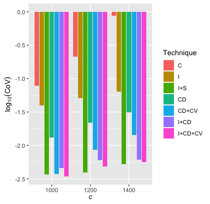
The simulation results are summarized in Table 3.1. A visual comparison of the CoV of different estimators is given in Figure 3.1.

To provide a reference point for comparing the estimators, we calculate the analytical result of the tail probability by

\[ \small{ \mathbf{P}(S>c) = \sum_{m=1}^{\infty} \mathbf{P}(M=m) \mathbf{P}(X_1+\cdots + X_m >c). }\]

This formula is calculable for this simple example because when \(X\sim\textrm{gamma}(a,b)\), \(X_1+\cdots + X_m \sim\textrm{gamma}(ma,b)\). Thus, the probabilities \(\mathbf{P}(X_1 +\cdots + X_m >c)\) for any \(m\) can be computed easily. For the infinite sum, we can truncate it at some value \(m_T\) such that \(\mathbf{P}(M>m_T)\) is small enough. In the example, \(M\sim \textrm{Poisson} (20)\), and we select \(m_T=400\) so that \(\mathbf{P}(M>m_T)\) is smaller than \(10^{-5}\). This means that our analytical result is accurate at least up to \(5\) decimal points.

In addition, for comparison, we provide the normal approximation of the tail probability, which is calculated by

\[\mathbf{P}(S>c) \simeq 1- \Phi \left(\frac{c-\mathbf{E}[S]}{\sqrt{\mathbf{Var} (S)}}\right),\]

where \(\Phi\) stands for the normal cumulative distribution function. We can see that normal approximation is not very accurate even for this simple example, especially when \(c\) is large.

As explained previously, estimators with smaller CoVs have smaller relative errors and, therefore, are better. Table 3.1 indicates that the combinations of importance sampling and stratified sampling (I+S); the conditioning method and the control variates method (CD+CV); importance sampling and the conditioning method (I+CD); and importance sampling, the conditioning method, and the control variates method (I+CD+CV) performed well. Methods involving importance sampling tend to have a small CoV when \(c\) is large. Therefore, they are recommended for simulating small tail probabilities.

4. Simulating mean excess loss

In this section, we introduce variance reduction methods for simulating the mean excess losses

\[\tau=\mathbf{E}[(S-c)_+].\]

4.1. Combining importance sampling and stratified sampling

The importance sampling method for simulating \(\tau\) is similar to that for \(\theta\): we simply replace \(\mathbb{I}(S^*>c)\) with \((S^*-c)_+\) in equation (3.1). This yields

\[ \hat{\tau}_I= (S^*-c)_+ {M_S(h)}{ \exp({-hS^*})}.\]

To combine importance and stratified sampling, we replace the function \(g_m^*\) in (3.4) with

\[g_m^*(x_1,\dots,x_m)= \left(\sum_{i=1}^m x_i - c\right)_+ {M_S(h)}{e^{- h\sum_{i=1}^m x_i}}.\]

4.2. The conditioning method

The following method for simulating the mean excess loss using the conditioning method was discussed by Peköz and Ross (2004). Define

\[A=\sum_{i=1}^{T(c)} X_i -c.\]

Then the conditional expectation estimator is constructed as

\[ \begin{aligned} \hat{\tau}_{C D} & =\mathbf{E}\left[(S-c)_{+} \mid {T}(c), {A}\right] \\ & =\sum_{i \geq {T}(c)}({A}+({i}-{T}(c)) \mathbf{E}[X]) \mathbf{P}[M=i] \\ & =({A}-{T}(c) \mathbf{E}[X]) \mathbf{P}[M \geq {T}(c)]\\ &\quad +\mathbf{E}[X] \mathbf{E}[M \mathbb{I}(M \geq {T}(c))] \\ & =({A}-{T}(c) \mathbf{E}[X]) \mathbf{P}[M \geq{ }T(c)]\\ &\quad +\mathbf{E}[X]\left(\mathbf{E}[M]-\sum_{{i}<{T}(c)} {i} \mathbf{P}[M=i]\right) \end{aligned} \]

The steps for implementing this simulation method are similar to those in Section 3.3; the only difference is that the value of \(A\) must be recorded in addition to \(T(c)\).

4.3. Combining the conditioning method and the control variates method

The following two control variates can be used to enhance the performance of the conditioning method without increasing computational efforts:

\[W_1=\sum\limits_{i=1}^{T(c)} (X_i-\mathbf{E}[X])\]

and

\[W_2=A-\mathbf{E}[A].\]

This yields the estimator

\[\hat{\tau}_{CD+CV} = \hat{\tau}_{CD}-\gamma_1W_1-\gamma_2W_2,\]

where \(\gamma_1\) and \(\gamma_2\) are chosen to minimize the variance of \(\hat{\tau}_{CD+CV}\). This could be achieved by setting the values of \(\gamma_1\) and \(\gamma_2\) to the least square estimate of the corresponding coefficients of the linear regression

\[\hat{\tau}_{CD}= \gamma_0+\gamma_1W_1+\gamma_2W_2+\epsilon,\]

where the values of \(\hat{\tau}_{CD}\), \(W_1\), and \(W_2\) are generated in simulation using the conditioning method.

For general discussions on least square or regression-based methods for using control variates, see the papers by Lavenberg and Welch (1981) and Davidson and MacKinnon (1992).

4.4. Combining importance sampling and the conditioning method

Similar to Section 3.5, importance sampling and the conditioning method can be combined. This results in the estimator

\[ \scriptsize{ \begin{align} &\hat{\tau}_{I+CD}\\ &\quad = \bigg[(A^*-T^*(c)\mathbf{E}[X])\mathbf{P}[M\geq T^*(c)]+\mathbf{E}[X]\mathbf{E}\left[M \mathbb{I}(M\geq T^*(c)) \right]\bigg]\frac{M_X(h)^{T^*(c)}}{e^{h\sum_{i=1}^{T^*(c)}X_i^*}} \end{align} }\]

where

\[A^*=\sum_{i=1}^{T^*(c)}X_i^*-c.\]

The proof of the unbiasedness of this estimator is given in Section A.2 of the Appendix.

Remark 4.1. The quantity \(\mathbf{E}[M \mathbb{I}(M\geq T^*(c))]\) is related to the size-biased transform (see Denuit 2020). We have

\[ \mathbf{E}[M \mathbb{I}(M\geq T^*(c))]= \mathbf{E}[M] \mathbf{P}[\tilde{M}\geq T^*(c)], \tag{4.1}\]

where \(\tilde{M}\) is the size-biased transform of \(M\) with distribution function

\[ \mathbf{P}[\tilde{M} = k]=\frac{k \mathbf{P}[M=k]}{\mathbf{E}[M]}, \quad k=0,1, \dots.\]

Equation (4.1) can be calculated efficiently because the distribution of \(\tilde{M}\) and \(M\) are often related. For example, as shown by Ren (2021), if \(M\) belongs to the \((a,b,0)\) class with parameter \((a,b)\), then \(\tilde{M}-1\) is in the \((a,b,0)\) class with parameter \((a,a+b)\). Particularly, if \(M\) follows the Poisson distribution with mean \(\lambda\), then \(\tilde{M}-1\) also follows the Poisson distribution with mean \(\lambda\). Therefore, for this case, (4.1) becomes

\[ \mathbf{E}[M \mathbb{I}(M\geq T^*(c))]= \lambda\mathbf{P}[M\geq T^*(c)-1],\]

which is straightforward to evaluate.

Remark 4.2. Control variates can be utilized to improve the results further. For example, let

\[W_1^*=\sum_{i=1}^{T^*(c)}(X_i^*-\mathbf{E}[X^*])\]

and

\[W_2^*=A^*-\mathbf{E}[A^*].\]

Then the estimator is

\[ \hat{\tau}_{I+CD+CV} = \hat{\tau}_{I+CD} - \gamma_1 W_1^* - \gamma_2 W_2^*,\]

where the values of \(\gamma_1\) and \(\gamma_2\) can be estimated by running the linear regression

\[\hat{\tau}_{I+CD}= \gamma_0+\gamma_1W_1^*+\gamma_2W_2^*+\epsilon.\]

4.2. Numerical experiments

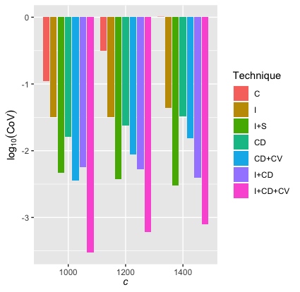
In this section, we compare the different methods for simulating \(\tau\) with the example set forth in Section 3.6. The results are shown in Table 4.1 and Figure 4.1.

In order to provide a reference point for the comparison, we list in the table values of \(\mathbf{E}[(S-c)_+]\) estimated using the importance sampling (I) method, but with a huge sample size of \(10^7\). These values are proxies for “analytical value” and labeled as “Target” in the table.

For this example, we did not provide the results for normal approximation of \(\mathbf{E}[(S-c)_+]\) because the approximation would not be accurate. The reason is that the normal approximation results for the tail probabilities are already inaccurate.

Table 4.1 and Figure 4.1 show that the combinations I+S, I+CD, and I+CD+CV have small CoVs and thus are efficient for estimating mean excess losses. In particular, the I+CD+CV method has by far the smallest CoV.

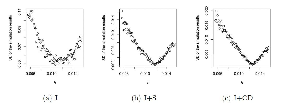
Remark 4.3. When carrying out the importance sampling methods, we have set the value of the tilting parameter to be the same as that for estimating the tail probability. That is, \(h\) is such that \(\mathbf{E}[S^*]=c\). However, this may not be the optimal choice.

For example, we have used \(h=0.009561118\) for the case of \(c=1200\) in the previous example. To explore the optimal value of \(h\), we experimented, and Figure 4.2 plots the SD of the estimator (based on repeating each method 100 times) against the values of \(h\). The figure shows that compared with the tail probability case, it may be preferable to set \(h\) to a greater value when estimating mean excess losses. Determining theoretical results for the optimal value of tilting parameter would be a great topic for future research.

5. Simulating tail probability: The two-dimensional case

In this section, we study methods for simulating the tail probability

\[\theta= \mathbf{P}[S_1>c, S_2>d]\]

for the two-dimensional compound variable \((S_1,S_2)\) defined in equation (1.4). The crude estimator is simply

\[\hat{\theta}_{0}= \mathbb{I}\left(S_1> c, \, S_2> d\right).\]

As in the one-dimensional case, this crude estimator has a large CoV and is inefficient. Therefore, we introduce several variance reduction methods to improve it.

5.1. Importance sampling

When using importance sampling to simulate \(\mathbf{P}[{S_1}>c, S_2>d]\), instead of sampling \(\mathbb{I}({S_1}>c, S_2>d)\), we sample

\[ \hat{\theta}_I = \mathbb{I}({S_1^*}>c, S_2^*>d) \frac{f(S_1^*, S_2^*)}{f^*(S_1^*, S_2^*)}, \tag{5.1}\]

where \((S_1^*, S_2^*)\) has a joint PDF \(f^*\). We assume that \(\mathbf{S}\) has finite moment generating function and choose \(\mathbf{S}^*\) to be the Esscher transform of \(\mathbf{S}\). That is,

\[f^*(x_1,x_2) = f(x_1,x_2) \frac{e^{h_1x_1+h_2x_2}}{M_{S_1, S_2}(h_1,h_2)} ,\]

where \(M_{S_1, S_2}(h_1,h_2)=\mathbf{E}[e^{h_1S_1+h_2S_2}]\) is the joint moment generating function of \((S_1, S_2)\). With this, (5.1) becomes

\[ \hat{\theta}_I = \mathbb{I}({S_1^*}>c, S_2^*>d) \frac{M_{S_1, S_2}(h_1,h_2)}{e^{h_1S_1^*+h_2S_2^*}}. \tag{5.2}\]

As in Section 3.1, we need to determine the value of the tilting parameters \((h_1,h_2)\) and a method to simulate \((S_1^*, S_2^*)\) in order to apply importance sampling.

Note 5.1. Similar to the one-dimensional case, we have

\[ \begin{align} \hat{\theta}_I&=\mathbb{I}(S_1^*>c, S_2^*>d) M_{S_1,S_2}(h_1,h_2)e^{-h_1S_1^*-h_2S_2^*}\\ &\leq M_{S_1,S_2}(h_1,h_2)e^{-h_1c-h_2d}. \end{align}\]

Then, a good choice for \((h_1,h_2)\) is to minimize the upper bound. To this end, taking the derivative of the upper bound on the right-hand side of the above equation with respect to \(h_1\) and \(h_2\) and setting to \(0\), we have

\[ \begin{align} c&=\frac{\frac{\partial}{\partial h_1}M_{(S_1,S_2)}(h_1,h_2)}{M_{(S_1,S_2)}(h_1,h_2)}\\ &=\frac{\mathbf{E}[S_1e^{h_1S_1+h_2S_2}]}{\mathbf{E}[e^{h_1S_1+h_2S_2}]}=\mathbf{E}[S_1^*], \end{align} \tag{5.3}\]

and

\[ d=\mathbf{E}[S_2^*]. \tag{5.4}\]

The values of \(h_1\) and \(h_2\) can be determined from (5.3) and (5.4).

The next note provides a representation of the distribution of \((S_1^*,S_2^*)\). The proof of this statement is given in Section A.3 of the Appendix.

Note 5.2. The Esscher transform of \(\mathbf{S}=(S_1, S_2)\) with parameter \((h_1,h_2)\) is

\[(S_1^*,S_2^*)=\bigg(\sum_{i=1}^{M^*} X_i^*,\sum_{j=1}^{N^*} Y_j^*\bigg),\]

where \(X^*\) and \(Y^*\) are the Esscher transforms of \(X\) and \(Y\) with parameters \(h_1\) and \(h_2\), respectively, and \((M^*,N^*)\) is the Esscher transform of \((M,N)\) with parameter \((\ln (M_X(h_1)),\ln (M_Y(h_2)))\).

In many important special cases, the distributions of \((S_1^*,S_2^*)\) and \((S_1,S_2)\) have similar structure, as the following examples show.

Example 5.1. Let \(\Lambda\sim \textrm{gamma}(\alpha,\beta)\). Conditional on \(\Lambda\), assume claim frequencies \(M\sim \textrm{Poisson}(\lambda_1\Lambda)\) and \(N\sim \textrm{Poisson}(\lambda_2\Lambda)\). Claim sizes \(X_i\), \(i=1,2, \dots\) are i.i.d. and follow a gamma distribution with parameters \((\alpha_1, \beta_1)\), and \(Y_j\), \(j=1,2, \dots\) are i.i.d. and follow a gamma distribution with parameters \((\alpha_2, \beta_2)\). With this setup, we have

\[ \small{ \begin{aligned} M_{S_1,S_2}(t_1,t_2)&=\mathbf{E}[e^{t_1S_1+t_2S_2}] \notag\\ &=\mathbf{E}_\Lambda \big[\mathbf{E}[e^{t_1S_1+t_2S_2}\mid \Lambda] \big]\notag\\ &=\mathbf{E}_\Lambda \big[ P_{M\mid\Lambda}\big(M_{X}(t_1)\big)\cdot P_{N\mid\Lambda}\big(M_{Y}(t_2)\big)\big]\notag\\ &=\mathbf{E}_\Lambda \big[ e^{\lambda_1\Lambda(M_X(t_1)-1)+\lambda_2\Lambda(M_Y(t_2)-1)}\big]\notag\\ &=M_\Lambda\big(\lambda_1(M_X(t_1)-1)+\lambda_2(M_Y(t_2)-1) \big)\notag\\ &=\bigg(1-\frac{\lambda_1M_X(t_1)+\lambda_2M_Y(t_2)-\lambda_1-\lambda_2}{\beta}\bigg)^{-\alpha}. \end{aligned} }\]

Therefore,

\[ \scriptsize{ \begin{aligned} &M_{S_1^*,S_2^*}(t_1,t_2)\\ &\quad=\frac{M_{S_1,S_2}(t_1+h_1,t_2+h_2)}{M_{S_1,S_2}(h_1,h_2)}\notag\\ &\quad=\bigg(1-\frac{\lambda_1M_X(t_1+h_1)+\lambda_2M_Y(t_2+h_2)-\lambda_1M_X(h_1)-\lambda_2M_Y(h_2)}{\beta+\lambda_1+\lambda_2-\lambda_1M_X(h_1)-\lambda_2M_Y(h_2)}\bigg)^{-\alpha}\notag\\ &\quad=\bigg(1-\frac{\lambda_1M_X(h_1)(\frac{M_X(t_1+h_1)}{M_X(h_1)}-1)+\lambda_2M_Y(h_2)(\frac{M_Y(t_2+h_2)}{M_Y(h_2)}-1)}{\beta+\lambda_1+\lambda_2-\lambda_1M_X(h_1)-\lambda_2M_Y(h_2)}\bigg)^{-\alpha}, \end{aligned} }\]

which implies that \((S_1^*,S_2^*)\) has the representation

\[(S_1^*, S_2^*) = \left(\sum_{i=1}^{M^*} X_i^*, \sum_{j=1}^{N^*} Y_j^*\right),\]

where \(\Lambda^*\sim\textrm{gamma}(\alpha,\beta+\lambda_1+\lambda_2-\lambda_1M_X(h_1)-\lambda_2M_Y(h_2))\) and, conditional on \(\Lambda^*\), \(M^*\sim \textrm{Poisson}(\lambda_1M_X(h_1)\Lambda^*), N^*\sim \textrm{Poisson}(\lambda_2M_Y(h_2)\Lambda^*)\). For the claim sizes, \(X_i^*\sim\textrm{gamma}(\alpha_1,\beta_1-h_1)\), and \(Y_j^*\sim\textrm{gamma}(\alpha_2, \beta_2-h_2)\).

This result means that \((S_1^*, S_2^*)\) is still a bivariate compound Poisson with common mixture and can easily be simulated.

Example 5.2. Suppose that the claim frequencies \(M\) and \(N\) have an additive common shock. That is, \(M=M_1+M_0\) and \(N= M_2+M_0\), where \(M_0\), \(M_1\), and \(M_2\) are independent. Let \(a=\ln (M_X(h_1))\) and \(b=\ln (M_Y(h_2))\), then

\[ (S_1^*, S_2^*) = \left(\sum_{i=1}^{M^*} X_i^*, \sum_{j=1}^{N^*} Y_j^*\right),\tag{5.5}\]

where \(M^*=M_1^*+M_0^*\) and \(N^*=M_2^*+M_0^*\), and where \(M_0^*, M_1^*\) and \(M_2^*\) are the Esscher transforms of \(M_0\), \(M_1\), and \(M_2\) with parameters \(a+b\), \(a\), and \(b\), respectively. In addition, \(X_i^*\) and \(Y_j^*\) are the Esscher transforms of \(X_i\) and \(Y_j\) with parameters \(h_1\) and \(h_2\).

This statement can be proved as follows.

Firstly,

\[ \scriptsize{ \begin{aligned} M_{S_1^*,S_2^*}(t_1,t_2) &=\frac{P_{M,N}(e^a M_{X^*}(t_1),e^b M_{Y^*}(t_2))}{P_{M,N}(e^a,e^b)}\notag\\ &=\frac{P_{M_1}(e^a M_{X^*}(t_1))}{P_{M_1}(e^a)}\frac{P_{M_2}(e^b M_{Y^*}(t_2))}{P_{M_2}(e^b)}\frac{P_{M_0}(e^{a+b}M_{X^*}(t_1)M_{Y^*}(t_2))}{P_{M_0}(e^{a+b})}. \end{aligned} }\]

Secondly,

\[ \small{ \begin{aligned} P_{M^*,N^*}(z_1,z_2)&=\mathbf{E}[z_1^{M^*}z_2^{N^*}]\notag\\ &=\mathbf{E}[z_1^{M_1^*}]\mathbf{E}[z_2^{M_2^*}]\mathbf{E}[(z_1z_2)^{M_0^*}]\notag\\ &=\frac{\mathbf{E}[e^{aM_1}z_1^{M_1}]}{\mathbf{E}[e^{aM_1}]}\frac{\mathbf{E}[e^{bM_2}z_2^{M_2}]}{\mathbf{E}[e^{bM_2}]}\frac{\mathbf{E}[e^{(a+b)M_0}(z_1z_2)^{M_0}]}{\mathbf{E}[e^{(a+b)M_0}]}\notag\\ &=\frac{P_{M_1}(e^a z_1)}{P_{M_1}(e^a)}\frac{P_{M_2}(e^b z_2)}{P_{M_2}(e^b)}\frac{P_{M_0}(e^{a+b}z_1z_2)}{P_{M_0}(e^{a+b})}. \end{aligned} }\]

Combining the above two equations, we have

\[M_{S_1^*,S_2^*}(t_1,t_2)=P_{M^*,N^*}(M_{X^*}(t_1),M_{Y^*}(t_2)),\]

which shows that \((S_1^*,S_2^*)\) has the compound representation of equation (5.5).

In particular,

• If \(M_0\sim \textrm{Poisson}(\lambda_0)\), \(M_1\sim \textrm{Poisson}(\lambda_1)\), and \(M_2\sim \textrm{Poisson}(\lambda_2)\), then
  \(M_0^*\sim \textrm{Poisson}(\lambda_0M_{X}(h_1)M_{Y}(h_2))\), \(M_1^*\sim \textrm{Poisson}(\lambda_1M_{X}(h_1))\), and

  \(M_2^*\sim \textrm{Poisson}(\lambda_2M_{Y}(h_2))\). Thus, \((M^*,N^*)\) follows a bivariate Poisson distribution with a common shock.

• If \(M_0\sim \textrm{NB}(r_0, p)\), \(M_1\sim \textrm{NB}(r_1,p)\), and \(M_2\sim \textrm{NB}(r_2,p)\), then

  \(M_0^*\sim \textrm{NB}(r_0,pM_{X}(h_1)M_{Y}(h_2))\), \(M_1^*\sim \textrm{NB}(r_1, pM_{X}(h_1))\), and \(M_2^*\sim \textrm{NB}(r_2, pM_{Y}(h_2))\). Thus \((M^*,N^*)\) no longer follows a bivariate negative binomial distribution. However, the pair can be easily simulated.

5.2. Combining importance sampling and stratified sampling

As in Section 3.2, we define

\[\small{\begin{align} &g_{m,n}^*(x_1,\dots,x_m,y_1,\dots,y_n)\\ &\quad = \frac{M_{(S_1,S_2)}(h_1,h_2)}{e^{h_1\sum_{i=1}^m x_i+h_2\sum_{j=1}^n y_j}} \mathbb{I}\left(\sum_{i=1}^m x_i >c, \sum_{j=1}^n y_j >d\right) \end{align}\tag{5.6}}\]

and

\[p_{m,n}^*=\mathbf{P}[M^*=m, N^*=n], \quad m,n=0,1,2,\dots,\]

where \((M^*, N^*)\) is the Esscher transform of \((M, N)\) with parameters \((\ln (M_X(h_1)), \ln (M_Y(h_2)))\). Then for given \(m_l, n_l\) such that \(1-\mathbf{P}[M^*\leq m_l, N^*\leq n_l]\) is small, an estimator for \(\mathbf{P}[S_1>c, S_2>d]\) is given by

\[\scriptsize{ \begin{aligned} \mathcal{E}&= \sum_{m=1}^{m_l}\sum_{n=1}^{n_l} g^*_{m,n}(X_1^*, \dots, X_{m}^*, Y_1^*,\dots,Y_{n}^*)p_{m,n}^*\notag\\ &\qquad+g^*_{m',n'}(X_1^*, \dots, X_{m'}^*,Y_1^*,\dots,Y_{n'}^*)\left(1-\sum_{m=0}^{m_l}\sum_{n=0}^{n_l}p_{m,n}^*\right). \end{aligned} \tag{5.7}}\]

To carry out the simulation, we simulate samples of \((M^*, N^*)\) conditional on at least one of them exceeding \((m_l, n_l)\). Supposing that the simulated values are \((m', n')\), we generate \(X_1^*, \dots, X_{\max(m_l,m')}^*\) and \(Y_1^*, \dots, Y_{\max(n_l,n')}^*\).

Denote \(m_l'= \max(m_l,m')\) and \(n_l'= \max(n_l,n')\). As in Section 3.2, a second estimator can be constructed as

\[ \scriptsize{ \begin{aligned} \mathcal{E}'&= \sum_{m=1}^{m_l}\sum_{n=1}^{n_l} g^*_{m,n}(X_{m_l'}^*, \dots, X_{m_l'-m+1}^*, Y_{n_l'}^*,\dots,Y_{n_l'-n+1}^*)p_{m,n}^*\notag\\ &\quad+g^*_{m',n'}(X_{m_l'}^*, \dots, X_{m_l'-m'+1}^*,Y_{n_l'}^*,\dots,Y_{n_l'-n'+1}^*)\\ &\qquad \times\left(1-\sum_{m=0}^{m_l}\sum_{n=0}^{n_l}p_{m,n}^*\right). \end{aligned}\tag{5.8} }\]

Combining them yields

\[\hat{\theta}_{I+S} = \frac{1}{2} (\mathcal{E}+\mathcal{E}'). \tag{5.9}\]

Remark 5.1. This method can be simplified if we choose \((m_l,n_l)\) so large that \(M_{(S_1,S_2)}(h_1,h_2)\) \((1-\mathbf{P}[M^*\leq m_l, N^*\leq n_l])\) is negligible. This way, as in Remark 3.1, the second term in (5.7) and (5.8) can be ignored. In addition, \(m_l'\) and \(n_l'\) in the first term of (5.8) are replaced by \(m_l\) and \(n_l\).

5.3. The conditioning method

The conditioning method introduced in Section 3.3 can be extended to the multivariate case as follows.

Let

\[T_1(c)=\min\bigg(m: \sum_{i=1}^{m} X_i >c\bigg)\]

and

\[T_2(d)=\min\bigg(n: \sum_{j=1}^{n} Y_j >d\bigg).\]

Then

\[\mathbb{I}(S_1>c, S_2>d) \Leftrightarrow \mathbb{I}( M\geq T_1(c), N\geq T_2(d)).\]

Hence,

\[\begin{aligned} &\mathbf{E}[\mathbb{I}(S_1>c, S_2>d) \mid T_1(c),T_2(d)]\\ &\quad =\mathbf{P}[M\geq T_1(c), N\geq T_2(d)\mid T_1(c), T_2(d)]\\ &\quad=\mathbf{P}[M\geq T_1(c), N\geq T_2(d)], \end{aligned}\]

where the last line is due to the fact that \((M,N)\) and \((T_1(c), T_2(d))\) are independent.

Consequently, an estimator for \(\theta\) using the conditioning method is \[\hat{\theta}_{CD}=\mathbf{P}[M\geq T_1(c), N\geq T_2(d)].\]

To implement the simulation, we first generate \(T_1(c)\) and \(T_2(d)\). If the generated values are \(t_{1,c}\) and \(t_{2,d}\), respectively, then \(\mathbf{P}[M\geq t_{1,c}, N\geq t_{2,d}]\) is the estimate for this run.

5.4. Combining the conditioning method and the control variates method

The conditioning method can be improved by applying control variates. For example, similar to the discussions in Section 4.3, we can introduce the control variates \[W_1=\sum\limits_{i=1}^{T_1(c)} (X_i-\mathbf{E}[X])\] and \[W_2= \sum\limits_{j=1}^{T_2(d)} (Y_j-\mathbf{E}[Y]),\] which are positively correlated with \(\hat{\theta}_{CD}\). The resulting estimator is \[\hat{\theta}_{CD+CV}=\hat{\theta}_{CD} -\gamma_1 W_1- \gamma_2 W_2,\] where the values of \(\gamma_1\) and \(\gamma_2\) are the least square estimate of the coefficients of the regression \[\hat{\theta}_{CD}= \gamma_0 + \gamma_1 W_1+ \gamma_2 W_2+\epsilon.\]

5.5. Combining importance sampling and the conditioning method

Let \(X_i^*\) and \(Y_j^*\) be the Esscher transforms of \(X_i\) and \(Y_j\) with parameters \(h_1\) and \(h_2\), respectively. Define \[T^*_1(c)=\min \bigg(m: \sum\limits_{i=1}^m X_i^*>c\bigg),\] \[T^*_2(d)=\min \bigg(n: \sum\limits_{j=1}^n Y_j^*>d\bigg),\] and \[S^*_{1,M}=\sum_{i=1}^M X_i^*,\] \[S^*_{2,N}=\sum_{j=1}^N Y_j^*.\]

We have the following estimator by combining importance sampling and the conditioning method.

\[\small{ \hat{\theta}_{I+CD}= \mathbf{P}[M\geq T_1^*(c), N\geq T_2^*(d)]\frac{M_X(h_1)^{T_1^*(c)}M_Y(h_2)^{T_2^*(d)}}{e^{h_1\sum_{i=1}^{T_1^*(c)}X_i^*+h_2\sum_{j=1}^{T_2^*(d)}Y_j^*}}. }\]

The proof of the unbiasedness of this estimator is provided in Section A.4 of the Appendix.

Remark 5.2. As in remark 4.2, control variates can be used to improve this method further. For example, we may use

\[W_1^*=\sum_{i=1}^{T_1^*(c)}(X_i^*-\mathbf{E}[X^*])\]

and

\[W_2^*=\sum_{j=1}^{T_2^*(d)}(Y_j^*-\mathbf{E}[Y^*]).\]

This leads to

\[ \hat{\theta}_{I+CD+CV} = \hat{\theta}_{I+CD} - \gamma_1 W_1^*- \gamma_2 W_2^*,\]

where the values of \(\gamma_1\) and \(\gamma_2\) can be estimated by running the regression

\[\hat{\theta}_{I+CD}= \gamma_0 + \gamma_1 W_1^*+ \gamma_2 W_2^* +\epsilon.\]

5.6. Numerical experiments

The goal of this section is to compare the different methods for simulating the tail probability \(\mathbf{P}(S_1>c, S_2>d)\).

We assume the following hypothetical distribution of \((S_1, S_2)\): Let \(\Lambda\sim \textrm{gamma}(10,0.5)\). Conditional on \(\Lambda\), claim frequencies \(M\) and \(N\) follow Poisson distributions with mean \(\Lambda\) and \(0.75\Lambda\), respectively. Claim severities \(X_i\) and \(Y_j\) follow gamma distributions with parameters \((20, 0.5)\) and \((30, 0.6)\), respectively.

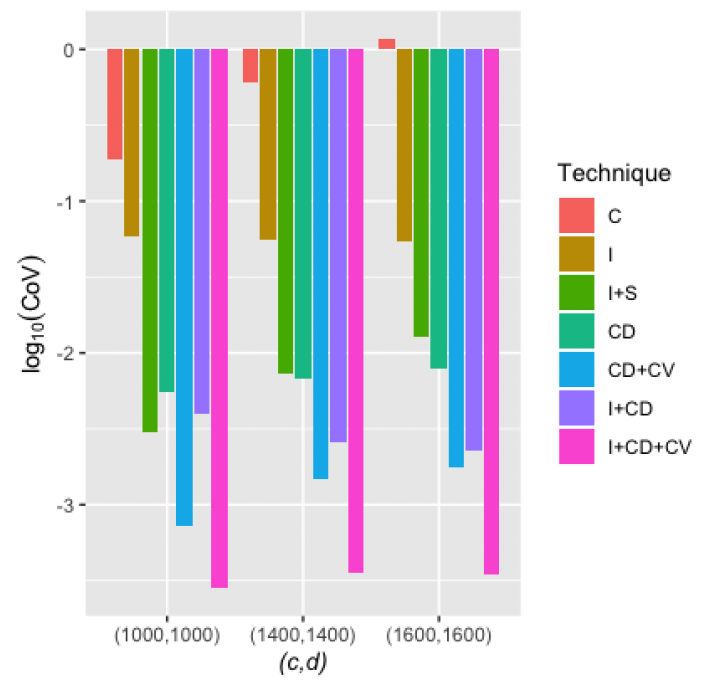
The numerical results of the simulations are reported in Table 5.1. A visual comparison of the CoVs of different estimators is given in Figure 5.1.

Similar to the univariate case, an estimator with a smaller CoV is better. The methods I+S, CD+CV, I+CD and I+CD+CV performed well.

To provide a reference point for comparing the estimators, the table also lists the analytical result of the tail probability calculated by

\[\begin{align} &\mathbf{P}(S_1>c, S_2>d) \\ &\quad = \sum_{m=1}^{\infty} \sum_{n=1}^{\infty} \mathbf{P}(M=m, N=n) \mathbf{P}\\ &\qquad \cdot (X_1+\cdots + X_m >c) \mathbf{P}(Y_1+\cdots + Y_n >d). \end{align}\]

This formula is calculable for this simple example because gamma distribution is closed under convolutions. Therefore, both \(X_1+\cdots+X_m\) and \(Y_1+\cdots+Y_n\) for all \(m\) and \(n\) follow gamma distributions. Consequently, all probabilities in the above equation can be easily evaluated. The infinite sum can be truncated at some value \((m_T, n_T)\) such that \(1-\mathbf{P}(M\le m_T, N\le n_T)\) is small enough. In the example, we select \(m_T=400\) and \(n_T=400\) so that \(1-\mathbf{P}(M\le m_T, N\le n_T)\) is smaller than \(10^{-5}\). As a result, our analytical result is accurate up to at least \(5\) decimal points.

Further, Table 5.1 reports the tail probability calculated through normal approximation of \((S_1, S_2)\). The approximation results are not accurate, especially at the tail.

6. Simulating mean excess loss: The two-dimensional case

In this section, we introduce variance reduction methods for simulating the bivariate mean excess losses

\[\tau=\mathbf{E}[(S_1-c)_+\times (S_2-d)_+].\]

6.1. Combining importance sampling and stratified sampling

To simulate \(\tau\) using importance sampling, we simply replace \(\mathbb{I}(S_1^*>c,S_2^*>d)\) in equation (5.2) with \((S_1^*-c)_+\times (S_2^*-d)_+\). This yields

\[ \hat{\tau}_I =(S_1^*-c)_+\times (S_2^*-d)_+ \frac{M_{S_1,S_2}(h_1,h_2)}{e^{ h_1S_1^*+h_2S_2^*}}.\]

To combine importance sampling and stratified sampling, we replace the function \(g_{m,n}^*\) in (5.6) with

\[ \small{ \begin{align} g_{m,n}^*(x_1,\dots,x_m,y_1,\dots,y_n)&= \left(\sum_{i=1}^m x_i - c\right)_+\\ &\quad \times \left(\sum_{j=1}^n y_j - d\right)_+ \frac{M_{S_1,S_2}(h_1,h_2)}{e^{ h_1\sum_{i=1}^m x_i+h_2\sum_{j=1}^n y_j}}. \end{align} }\]

6.2. Combining the conditioning method and the control variates method

We use the notation in Section 5.3 and, in addition, for \(k\ge 1\), let \(S_{1,k}=\sum_{i=1}^{k} X_i\) and \(S_{2,k}=\sum_{i=1}^{k} Y_i\). Define

\[A=S_{1, T_1(c)}-c\] and \[B=S_{2, T_2(d)}-d.\]

Then, since

\[ \scriptsize{\tau=\mathbf{E}\bigg[\sum_i\sum_j (S_{1,i}-c)^+(S_{2,j}-d)^+\mathbf{P}[M=i,N=j]\bigg],}\]

an estimator for \(\tau\) using the conditioning method is

\[ \scriptsize{ \hat{\tau}_{CD}= \mathbf{E}\bigg[\sum_i\sum_j (S_{1,i}-c)^+(S_{2,j}-d)^+\mathbf{P}[M=i,N=j]\mid T_1(c),T_2(d),A,B \bigg]. }\]

After simulating the values of \(T_1(c),T_2(d),A\), and \(B\), \(\hat{\tau}_{CD}\) can be evaluated as follows:

\[ \scriptsize{ \begin{aligned} \hat{\tau}_{CD} &= \mathbf{E}\bigg[\sum_i\sum_j (S_{1,i}-c)^+(S_{2,j}-d)^+\mathbf{P}[M=i,N=j]\mid T_1(c),T_2(d),A,B \bigg]\notag\\ &=\sum_{i\geq T_1(c)}\sum_{j\geq T_2(d)}(A+(i-T_1(c))\mathbf{E}[X])(B+(j-T_2(d))\mathbf{E}[Y])\mathbf{P}[M=i,N=j]\notag\\ &=(A-T_1(c)\mathbf{E}[X])(B-T_2(d)\mathbf{E}[Y])\mathbf{P}[M\geq T_1(c),N\geq T_2(d)]\notag\\ &\quad+(B-T_2(d)\mathbf{E}[Y])\mathbf{E}[X]\sum_{i\geq T_1(c)}\sum_{j\geq T_2(d)}i\mathbf{P}[M=i,N=j]\notag\\ &\quad +(A-T_1(c)\mathbf{E}[X])\mathbf{E}[Y]\sum_{i\geq T_1(c)}\sum_{j\geq T_2(d)}j\mathbf{P}[M=i,N=j]\notag\\ &\quad+\mathbf{E}[X]\mathbf{E}[Y]\sum_{i\geq T_1(c)}\sum_{j\geq T_2(d)}ij\mathbf{P}[M=i,N=j]. \end{aligned}\tag{6.1} }\]

Remark 6.1. Equation (6.1) shows that when using the conditioning method, the problem of estimating the tail mean of the aggregate loss \((S_1, S_2)\) is replaced by the problem of computing the tail mean of the claim frequencies \((M,N)\). Note that the infinite sum needs to be evaluated carefully. In this paper, we simply truncate the sum to very large value of \(i\) and \(j\).

The estimator \(\hat{\tau}_{CD}\) can be improved by introducing some control variates. For example, using \[W_1=\sum\limits_{i=1}^{T_1(c)} (X_i-\mathbf{E}[X]),\] \[W_2=\sum\limits_{j=1}^{T_2(d)} (Y_j-\mathbf{E}[Y]),\] \[W_3=A-\mathbf{E}[A],\] and \[W_4=B-\mathbf{E}[B]\] results in the estimator \[\hat{\tau}_{CD+CV}=\hat{\tau}_{CD} -\gamma_1 W_1- \gamma_2 W_2-\gamma_3 W_3- \gamma_4 W_4,\] where the parameters \(\gamma_1, \gamma_2, \gamma_3\), and \(\gamma_4\) can be determined by fitting the linear regression model \[\hat{\tau}_{CD} = \gamma_0+\gamma_1W_1+\gamma_2W_2+\gamma_3W_3+\gamma_4W_4+\epsilon.\]

6.3. Combining importance sampling and the conditioning method

We use the notation in Section 5.5 and, further, define

\[A^*=S^*_{1,T_1^*(c)}-c\]

and

\[B^*=S^*_{2,T_2^*(d)}-d.\]

Then,

\[\scriptsize{ \begin{aligned} \hat{\tau}_{I+CD} &=\bigg(\big(A^*-T_1^*(c)\mathbf{E}[X]\big)\big(B^*-T_2^*(d)\mathbf{E}[Y]\big)\mathbf{P}[M\geq T_1^*(c), N\geq T_2^*(d)]\notag\\ &\quad +\mathbf{E}[X]\big(B^*-T_2^*(d)\mathbf{E}[Y]\big)\mathbf{E}\big[M\mathbb{I}(M\geq T_1^*(c),N\geq T_2^*(d))\big]\notag\\ &\quad+\mathbf{E}[Y]\big(A^*-T_1^*(c)\mathbf{E}[X]\big)\mathbf{E}[N\mathbb{I}(M\geq T_1^*(c),N\geq T_2^*(d))]\notag\\ &\quad +\mathbf{E}[X]\mathbf{E}[Y]\mathbf{E}\big[MN\mathbb{I}(M\geq T_1^*(c),N\geq T_2^*(d))\big]\bigg)\frac{M_X(h_1)^{T_1^*(c)}M_Y(h_2)^{T_2^*(d)}}{e^{h_1\sum_{i=1}^{T_1^*(c)}X_i^*+h_2\sum_{j=1}^{T_2^*(d)}Y_j^*}}. \end{aligned} }\]

The expectations in the above equation can be evaluated by their definitions. For example, we have

\[\begin{align} &\mathbf{E}[M\mathbb{I}(M\geq T_1^*(c),N\geq T_2^*(d))]\\ &\quad= \sum_{i\geq T_1^*(c)}\sum_{j\geq T_2^*(d)}i\mathbf{P}[M=i,N=j]. \end{align}\]

The unbiasedness of this estimator is shown in Section A.5 of the Appendix.

Remark 6.2. Control variates can be introduced to improve the estimator further. For example, we may use

\[W_1=\sum_{i=1}^{T_1^*(c)}(X_i^*-\mathbf{E}[X^*]),\]

\[W_2=\sum_{j=1}^{T_2^*(d)}(Y_j^*-\mathbf{E}[Y^*]),\]

\[W_3=A^*-\mathbf{E}[A^*], and\]

\[W_4=B^*-\mathbf{E}[B^*].\]

This leads to the estimator

\[\hat{\tau}_{I+CD+CV}=\hat{\tau}_{I+CD} -\gamma_1 W_1- \gamma_2 W_2-\gamma_3 W_3- \gamma_4 W_4,\]

where the parameters \(\gamma_1, \gamma_2, \gamma_3\), and \(\gamma_4\) can be determined by fitting the linear regression

\[\hat{\tau}_{I+CD} = \gamma_0+\gamma_1W_1+\gamma_2W_2+\gamma_3W_3+\gamma_4W_4+\epsilon.\]

6.4. Numerical experiments

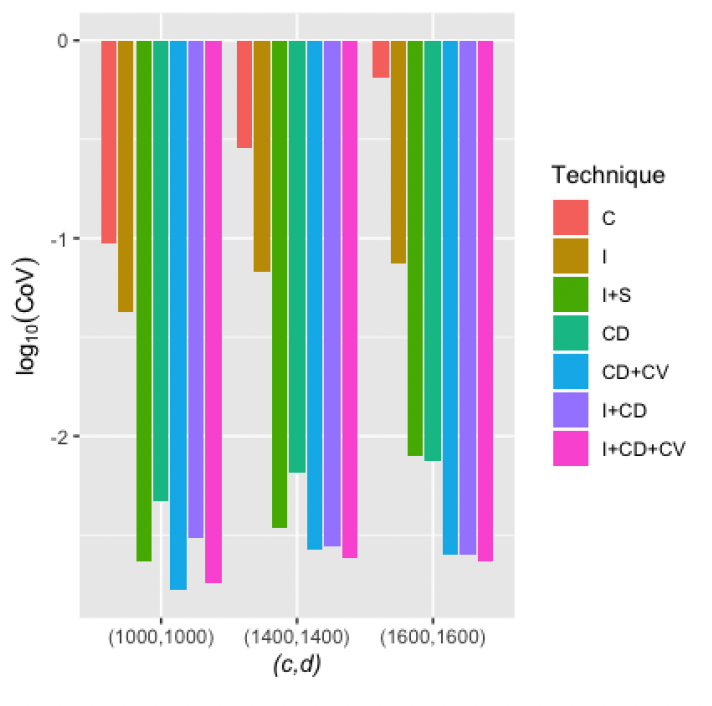
We simulated the tail mean for the example set forth in Section 5.6, and the results are reported in Table 6.1 and Figure 6.1. The “Target” values of \(\mathbf{E}[(S_1-c)_+\times(S_2-d)_+]\) are estimated by the importance sampling method with a huge sample size of \(10^7\). They are the proxies for the true values.

The I+CD+CV method has the smallest relative error among all methods introduced.

7. Conclusion

Methods for simulating tail probability and tail mean of both univariate and bivariate compound variables were studied in detail in this paper. We first reviewed some basic simulation variance reduction methods, then we proposed several novel combinations of variance reduction methods specifically for compound distributions. We showed that combinations of importance sampling, stratified sampling, the conditioning method, and the control variates method can greatly enhance the performance of the preliminary methods in estimating tail probability and tail mean. Among all the methods we studied, the I+CD+CV combination consistently performed well, with its CoV (relative error) among the smallest of all methods in all experiments. This combination is especially helpful for simulating the tail mean.

We have proposed the simulation methods for some simple and commonly used aggregate loss models. In practice, the scenarios that need to be simulated are much more complex and the methods introduced here may not be directly used. However, it is likely that the basic variance reduction methods and their combinations can still be applied after some adaptations to the actual problem. We argue that it is worthwhile for actuaries to spend the time and energy to discover ways to utilize them because they could enhance the accuracy of simulations and/or significantly reduce simulation times.

---

Acknowledgments

The authors are grateful to two anonymous reviewers for their valuable comments, which helped improving the paper greatly. We also appreciate the many discussions on the topic with Professors Edward Furman, Katsu Goda and Ricardas Zitikis. This research has been supported by the Natural Sciences and Engineering Research Council (NSERC) of Canada.