On the Importance of Dispersion Modeling for Claims Reserving: An Application with the Tweedie Distribution

1. Introduction

Setting an appropriate claims reserve is one of the main tasks of non-life actuaries. Many methods have been developed for such purposes, among which the most extensively used are the chain-ladder, the Bornhuetter-Ferguson, and generalized linear models (GLMs). One can refer to Wüthrich and Merz (2008) and England and Verrall (2002) for a complete survey of the topic.

The establishment of claims reserves comprises two main objectives: determining a good point estimate, and evaluating the uncertainty around that point. The literature is littered with a wide variety of models. Even though some might agree on similar point estimates, it is not uncommon to find models that predict significantly different reserve uncertainty levels. In this context, choosing the right model might become problematic for the practitioner as his decision might greatly affect the financial statements of the company, especially since the introduction of Solvency II. In order to better understand the variance of the model and reduce the gap of the predicted variances between models, this paper proposes ways to model both the mean of the costs and their dispersion.

In a GLM framework, when a model focuses only on the mean of the costs, the predicted variance is usually considered in a left-over calculation that only depends on the corresponding predicted mean, up to a constant. Consequently, depending on the mean-variance relationship and the dispersion parameter, two different models can attribute different variances to the same predicted mean. Therefore, the overall predicted variances from model to model can be significantly different, while the overall point estimate remains relatively similar. However, if a flexible variance structure is introduced, different models will tend to agree a little more on the variance of each observation, thus reducing the gap in the reserve uncertainty levels between models.

Moreover, and more importantly, there is a strong indication that some practical cases require a flexible variance structure in order to capture the underlying risk appropriately. These occur mainly when the frequency and severity trends move in opposite directions. An example of such a situation is shown in Section 3.

We then show that a flexible variance structure can be incorporated with a direct MLE estimation or with a double generalized linear model (DGLM). In a known frequency framework, both approaches give the exact same results. In an unknown frequency framework, there is little difference originating in the ² approximation for the DGLM. Finally, we also introduce a variance correction that takes into account the downward bias of the maximum likelihood estimators.

As a starting point, we consider the constant dispersion model from Wüthrich (2003), which is described in Section 2. Section 3 depicts potential flaws of this model in some practical situations. Two types of models that incorporate variance modeling are presented in Section 4. Finally, an application of these models is illustrated in Section 5, followed by a discussion.

2. Tweedie’s distribution

This section closely follows Wüthrich (2003) . Assume that the data is displayed in a triangle, the accident years are denoted by $i \leq I$, and the development periods are denoted by $j \leq J$. Let $C_{i, j}$ denote the random variable that represents the incremental payments for claims with origin in accident year $i$ during the development period $j$. Suppose that $w_{i, j}$ is the exposure of cell $(i, j)$. There are several ways to choose an appropriate exposure: the premium volume of the accident year, the number of policies, etc. We are interested in modeling the normalized incremental payments, denoted by $Y_{i, j}=\frac{C_{i, j}}{w_{i, j}}$. Additionally, suppose that

1. The number of payments $R_{i, j}$ are independent and Poisson distributed with mean $\lambda_{i, j} w_{i, j}$. We will denote $r_{i, j}$ the realization of $R_{i, j}$.

2. The individual payments $X_{i, j}^{(k)}$ are independent and gamma distributed with mean $\tau_{i, j}$ and shape parameter $\nu>0$.

3. $R_{i, j}$ and $X_{m, n}^{(k)}$ are independent for all indices.

4. $C_{i, j}=1_{\left\{R_{i, j}>0\right\}} \sum_{k=1}^{R_{i, j}} X_{i, j}^{(k)}$

As shown in Appendix A of Wüthrich (2003), $Y_{i, j}$ follows a Tweedie’s compound Poisson model. Moreover, the distribution of $Y_{i, j}$ can also be reparametrized in such a way that it takes the form of the exponential dispersion family:

$$\begin{aligned} p & =\frac{\nu+2}{\nu+1}, \quad p \in(1,2), \\ \mu_{i, j} & =\lambda_{i, j} \tau_{i, j} \\ \phi_{i, j} & =\frac{\lambda_{i, j}^{1-p} \tau_{i, j}^{2-p}}{(2-p)} \end{aligned}$$

so that Y i, j has a probability weight at 0 given by

$$\begin{aligned} P\left(Y_{i, j}=0\right) & =P\left(R_{i, j}=0\right) \\ & =\exp \left\{-w_{i, j} \lambda_{i, j}\right\}=\exp \left\{\frac{w_{i, j}}{\phi_{i, j}}\left(-\kappa_{p}\left(\theta_{i, j}\right)\right)\right\} \end{aligned}$$

and for y 0,

$$\begin{array}{l} f_{Y_{i, j}}\left(y \mid \lambda_{i, j}, \tau_{i, j}, \nu\right) d y \\ =c\left(y ; \frac{w_{i, j}}{\phi_{i, j}} ; p\right) \exp \left\{\frac{w_{i, j}}{\phi_{i, j}}\left(y \theta_{i, j}-\kappa_{p}\left(\theta_{i, j}\right)\right)\right\} d y, \end{array} \tag{2.1}$$

where

$$\begin{aligned} \theta_{i, j} & =\theta\left(\mu_{i, j}\right)=\frac{\mu_{i, j}^{1-p}}{1-p}<0, \\ \kappa_{p}\left(\theta_{i, j}\right) & =\frac{\mu_{i, j}^{2-p}}{2-p}=\frac{1}{2-p}\left((1-p) \theta_{i, j}\right)^{\frac{2-p}{1-p}}, \\ c\left(y ; \frac{w_{i, j}}{\phi_{i, j}} ; p\right) & =\sum_{r \geq 1}\left(\frac{y^{\nu}\left(w_{i, j} / \phi_{i, j}\right)^{\nu+1}}{(p-1)^{\nu}(2-p)}\right)^{r} \frac{1}{r ! \Gamma(\nu r) y} . \end{aligned}$$

We also suppose that the means follow a multiplicative structure so that

$$\mu_{i, j}=\exp \left\{X_{i, j} \beta\right\}$$

where β are the mean parameters and X i, j are the cell coordinates of observation (i, j). Then, as shown in Jørgensen (1997), the mean and variance of Y i, j are given by

$$\begin{array}{c} \mathrm{E}\left[Y_{i, j}\right]=\mu_{i, j}\left(=\kappa_{p}^{\prime}\left(\theta_{i, j}\right)=\frac{\partial\left(\kappa_{p}\left(\theta_{i, j}\right)\right)}{\partial \theta_{i, j}}\right), \\ \operatorname{Var}\left[Y_{i, j}\right]=\frac{\phi_{i, j}}{w_{i, j}} \mu_{i, j}^{p}\left(=\frac{\phi_{i, j}}{w_{i, j}} \kappa_{p}^{\prime \prime}\left(\theta_{i, j}\right)\right). \end{array}$$

We say that $Y_{i, j}$ has mean $\mu_{i, j}$, exposure $w_{i, j}$, dispersion parameter $\phi_{i, j}$, and the power of the variance function is $p$. The boundary cases $p \rightarrow 1$ and $p \rightarrow$ 2 correspond to the overdispersed Poisson and the gamma models, respectively. Hence, Tweedie’s compound Poisson model with $p \in(1,2)$ can be seen as a bridge between the Poisson and the gamma models. Although the Tweedie class of models is defined on almost all the real values of $p$, this paper considers only $p \in(1,2)$.

2.1. Likelihood function

Using the density of Equation (2.1), we get the following log-likelihood function:

$$\begin{aligned} l=\sum_{i, j}\left(\operatorname { l o g } \left(c \left(y_{i, j}\right.\right.\right. & \left.\left.; \frac{w_{i, j}}{\phi_{i, j}} ; p\right)\right) \\ & \left.+\frac{w_{i, j}}{\phi_{i, j}}\left(y_{i, j} \frac{\mu_{i, j}^{1-p}}{1-p}-\frac{\mu_{i, j}^{2-p}}{2-p}\right)\right) . \end{aligned} \tag{2.2}$$

2.2. Dispersion parameter

The dispersion parameter can be estimated in at least two ways. The first approach is the maximum likelihood estimator. Setting the first derivatives of the log-likelihood (2.2) equal to 0, one gets (for $\phi_{i, j}$ constant):

$$\phi_{i, j} \equiv \phi=\frac{-\Sigma_{i, j} w_{i, j}\left(y_{i, j} \frac{\mu_{i, j}^{1-p}}{1-p}-\frac{\mu_{i, j}^{2-p}}{2-p}\right)}{(1+\nu) \Sigma_{i, j} r_{i, j}} .$$

The second approach uses the deviance principle. This measure compares the likelihood of a model resulting in means $\left(\mu_{i, j}\right)$ to an unrestricted full model $\left(y_{i, j}\right)$, as shown below:

$$D=2\left(l\left(\mu_{1,1}, \mu_{2,1}, \cdots, \mu_{1, J}\right)-l\left(y_{1,1}, y_{2,1}, \cdots, y_{1, J}\right)\right)$$

Adjusting for the number of parameters in the model, one gets the following deviance estimator (for $\phi_{i, j}$ constant):

$$\phi_{i, j} \equiv \phi=\sum_{i, j} \frac{2}{N-Q}\left(y_{i, j} \frac{y_{i, j}^{1-p}-\mu_{i, j}^{1-p}}{1-p}-\frac{y_{i, j}^{2-p}-\mu_{i, j}^{2-p}}{2-p}\right)$$

where N is the number of observations and Q is the number of parameters used to estimate the means.

2.3. Optimizing p

Regardless of which principle one uses to determine $\phi$, the variance parameters ($p$ and $\phi$) need to be estimated at the same time. As shown in Wüthrich (2003), the variance parameters have a limited impact on the mean parameters and vice-versa. Indeed, $p, \phi$, and to some extent $w_{i, j}$, tend to have their main influence on the variance of the model, and less so on the means. Similarly, the means have only an indirect impact on the variances.

When using the likelihood principle for estimating , one can replicate the algorithm shown in Wüthrich (2003), which alternates the optimization between the means and the variances. However, there is an even quicker approach: one can use the built-in optimization algorithms of statistical computer programs to estimate both the mean and the variance parameters at the same time.

2.4. Mean squared error of prediction

The reserve uncertainty level is typically measured by the mean squared error of prediction (MSEP). It is common to decompose this statistic in two:

$$\text { MSEP }=\text { Process risk }+ \text { Parameter estimation error }$$

The process risk describes the fluctuation of random variables getting various outcomes for each realization. The parameter error reflects the uncertainty in the reliability of the estimates of the parameters. One can find a good explanation about the MSEP for Tweedie models in Peters, Shevchenko, and Wüthrich (2009). Using the same approach as described in Wüthrich (2003), the MSEP of a Tweedie compound Poisson model as defined previously can be approximated by

$$\begin{aligned} \operatorname{MSEP}[R] \approx & \sum_{(i, j) \in \Delta} \phi w_{i, j} \mu_{i, j}^{p} \\ & +\sum_{(i, j) \in \Delta}\left(w_{i, j} \mu_{i, j}\right)^{2} \operatorname{Var}\left[\eta_{i, j}\right] \\ & +\sum_{(i, j) \in \Delta,\left(i_{1}, j_{1}\right) \neq\left(i_{2}, j_{2}\right)}\left(w_{i_{1}, j_{1}} \mu_{i_{1}, j_{1}}\right)\left(w_{i_{2}, j 2} \mu_{i_{2}, j_{2}}\right) \\ & \operatorname{Cov}\left(\eta_{i_{1} j_{1}} \eta_{i 2 j 2}\right) . \end{aligned} \tag{2.3}$$

where $R$ is the total reserve, which is the sum of the future predicted incremental claims, and $\Delta$ represents the cell coordinates of future claims. Also, $\eta_{i, j} =X_{i, j} \beta$ and $\operatorname{Cov}\left(\boldsymbol{\eta}_{i_1 j_1}, \eta_{i_2 j_2}\right)$ denotes the sum of the covariance matrix elements intersecting the two sets of parameters. One can refer to England and Verrall (2002) for more details.

3. Variance modeling

Although dispersion modeling has seen many applications (see Smyth and Jørgensen 2002), it is not yet thoroughly covered in the context of claims reserving. Still, there are a few discussions on this topic, namely section 8.1 of Taylor (2000), albeit that heteroscedasticity is treated there by means of weights. In a chain ladder framework, Mack’s (1993) model has a natural tendency to have a flexible variance structure since the $\sigma_j^2$ are estimated for each column. In a Tweedie model context, there is some evidence in Wüthrich (2003) that this topic has been attentively considered, yet, there has not been a follow-up work to support that idea. This notion also emerges once again a few years later in England and Verrall (2006), when an estimator of the dispersion parameter for each column in the bootstrap algorithm is developed. As of late, there are two more papers on the Tweedie model that apply a varying dispersion parameter: Taylor and University of Melbourne (2007) Section 4, Equation (4.1), and Meyers (2008) Section 3, Equation 4, and footnote 1. Still, there might be indications that variance modeling can be explored further in a Tweedie model framework.

Before introducing a GLM structure that accounts for both the mean and the dispersion, one needs to understand the phenomenon encountered in practice that triggers this need. To begin, it is not uncommon to come upon situations where most of the claims are declared early in the development years. In this case, we say that there is a decreasing tendency for the frequency throughout the development years. On the other hand, there exist situations where the average cost of claims tends to get bigger throughout the development periods. For example, in the automobile business line, when an accident benefit^[1] claim goes to court, the longer the trial lasts, the greater the potential size of the claim. Hence, claim severity can have a positive trend. The modeling key is to recognize a situation where the frequency has one trend, and the severity has the opposite trend, regardless of which is going up or down. These are the situations where models with constant dispersion are most prone to mishandling the variance of the risk.

A good way to deal with such situations is to model separately the frequency and the severity and to combine them only in the end. This observation has already been made by Adler and Kline (1978), which incorporates these notions by the use of a deterministic approach. Similar approaches can be also found in de Jong and Zehnwirth (1983), Reid (1978), and Wright (1990).

Alternatively, one can argue that a Tweedie’s compound Poisson model is by definition a good way to take into account both the frequency and the severity. Indeed, the model has a good structure; however, the number of parameters used to describe the risk can be insufficient. To picture this, one can analyze the following typical situation. Suppose that the aggregate losses C follow a standard compound Poisson model:

$$C=\sum_{k=1}^{N} X_{k}$$

where $N$ is Poisson distributed, $X_k$ is gamma distributed, and $X_k$ and $N$ are independent for all indices. One can calculate the first two moments of $C$ as shown in Table 1 (Case 1). Now, we are interested in what happens if we double the frequency as opposed to doing the same to the severity. Without any surprises, in both cases, the mean of the total costs doubles. However, the variance quadruples in Case 3 while it only doubles in Case 2. This situation forces a Tweedie model with constant dispersion factor to choose a predicted variance that has the potential to be correct at most in only one of the two scenarios. Therefore, depending on the information on the frequency and the severity, the total claims model might need additional parameters in order to be correctly adjusted for its variance.

In the same spirit, the optimization of p helps the variance structure to better replicate the uncertainty of the risk without affecting the means noticeably. It is a known feature that the p parameter is strongly correlated with the overall importance of the severity in the model. If there are many small claims (pre-dominant frequency), p will be closer to 1 (Poisson model). Inversely, if there are a few large gamma-distributed claims, p will tend towards 2 (gamma model). Finally, one should keep in mind that the p parameter is deeply related to the dispersion parameters and has an important impact on the variance of the model.

One could argue that we could incorporate a flexible model structure $p_{i, j}$ instead of using a flexible variance structure $\phi_{i, j}$. Indeed, this could be explored; however, one first needs to prove that the flexible variance structure is insufficient. Second, developing an analytic formula for a flexible $p_{i, j}$ can be very hard, even impossible, and it is needless to say that numerical approximations could have convergence problems. Third, the Tweedie class of models tends to be quite different for $p \notin(1,2)$, which might trigger additional difficulties. For all of the above reasons, we suppose that $p$ is constant (but still needs to be estimated).

4. Dispersion models

4.1. Defining a flexible variance structure

A dispersion model has a flexible variance structure denoted by

$$\phi_{i, j}=\exp \left\{Z_{i, j} \gamma\right\}$$

where $\phi_{i, j}$ is the dispersion factor of cell $(i, j)$ and $Z_{i, j}$ is the $(i, j)^{t h}$ row of the design matrix with the corresponding vector of parameters $\gamma$. We use rows and columns to explain the dispersion just as we would for the means.

To establish a flexible variance structure in the model, we insert $\phi_{i, j}$ in the likelihood function (2) instead of $\phi$. Unfortunately, this procedure differs somewhat, depending on whether we know the underlying frequency or not. When the number of claims is known, the infinite sum in the likelihood function reduces to one term only (the observed frequency), which greatly simplifies the calculations. In the latter case, the presence of the infinite series makes the procedure complex. One way to approximate it is by recognizing a generalized Bessel function as shown in Peters, Shevchenko, and Wüthrich (2009). An alternate approach would be to use the saddle-point approximation as suggested in Jørgensen (1997). This paper’s main focus is the application of dispersion models in a known frequency framework, and thus the technical difficulties emerging from an unknown frequency framework are not discussed here.

Two approaches are explored to maximize the likelihood: direct estimation through the maximum likelihood estimators (ML) and the double generalized linear model (DGLM). First, the ML estimators are obtained through direct optimization of the likelihood function. This can be done with the use of a statistical package or by setting the first derivatives of the likelihood function equal to zero.

A DGLM comprises two distinct general linear submodels that are calibrated successively until global convergence is met. We usually define one submodel for the means and the other submodel for the variances. Both submodels communicate to each other through response variables. Depending on whether we know the frequency or not, the required response variables can be different. When the frequency is unknown, we have a joint mean-variance model that is part of the exponential dispersion family. This allows the use of the unit deviances of the means as a response for the variance submodel, which in turn generates the dispersion used to calibrate the exposures of the mean submodel.

On the other hand, when the number of claims is known, the joint mean-variance likelihood function simplifies in such a way that it unfortunately excludes the model from the exponential dispersion family. This disallows the use of straight unit deviances as response variables and thus triggers the need of a clever transformation to restore the DGLM framework (see Section 4.2.2).

Since the ML and the DGLM aim for the same objective, their optimal parameters are usually very alike or even exactly the same. In fact, in an unknown frequency framework, since an approximation for the likelihood is required, the results might not be exactly the same as the ML. On the other hand, when the number of claims is known, the ML and DGLM give exactly the same results, as there is no approximation at all (see Section 4.2.2).

Models with a flexible variance structure are more prone to have technical difficulties such as over-parametrization, as foreshadowed in Wüthrich (2003) (Section 4.2). For example, one often cannot use explicit variance parameters near the ends of the triangle because the observations get scarce. Therefore, one should either regroup the last few lines together, or use tendency parameters instead (Hoerl’s curve). Additionally, one should be aware of the possible bias created when regrouping the last lines of the triangle together. Since the means are disproportionably well estimated near the ends of the triangle, the dispersion might be somewhat flawed in these regions.

4.2. Estimation with a known frequency

4.2.1. Maximum likelihood estimation

The maximum likelihood estimates are obtained through direct optimization of the likelihood function. Using Equation (2.2) and known frequency $r_{i, j}$, the log-likelihood function becomes:

$$\begin{aligned} l= & \sum_{i, j} r_{i, j} \log \left(\frac{\left(w_{i, j} / \phi_{i, j}\right)^{\nu+1} y_{i, j}^{\nu}}{(p-1)^{\nu}(2-p)}\right)-\log \left(r_{i, j} ! \Gamma\left(r_{i, j} \nu\right) y_{i, j}\right) \\ & +\frac{w_{i, j}}{\phi_{i, j}}\left(y_{i, j} \frac{\mu_{i, j}^{1-p}}{1-p}-\frac{\mu_{i, j}^{2-p}}{2-p}\right) . \end{aligned} \tag{4.1}$$

Although the log-likelihood function (4.1) is no longer part of the exponential family (Smyth and Jørgensen 2002), the optimization is easier to obtain because there is no infinite series to approximate. Also, it is important to note that knowing the frequency impacts mostly the variances of the claim costs since the means were already well modeled.

4.2.2. DGLM estimation

We closely follow the methodology described in Smyth and Jørgensen (2002) which contains the complete demonstration for all the results presented in this section. In order to be able to use the DGLM when the frequency is known, we need to define dispersion-prior exposures as:

$$\left(w_{d}\right)_{i, j}=\frac{2 w_{i, j} \mu_{i, j}^{2-p}}{(2-p)(p-1) \phi_{i, j}}$$

and dispersion-responses as

$$d_{i, j}=-\frac{2}{\left(w_{d}\right)_{i, j}}\left(\frac{r_{i, j} \phi_{i, j}}{p-1}+w_{i, j}\left(y_{i, j} \frac{\mu_{i, j}^{1-p}}{1-p}-\frac{\mu_{i, j}^{2-p}}{2-p}\right)\right)$$

For each submodel, the Fisher scoring equations are used to find the optimal parameters. First, the mean gets optimized using a Tweedie model with a fixed deviance and fixed $p$. Then the deviance-responses are optimized using the saddle-point approximation which supposes that the $d_{i, j}$ are approximately distributed, as $\phi_{i, j} \chi_1^2$ for $\phi_{i, j}$ is reasonably small. Since this distribution is a particular case of the gamma distribution (with its own dispersion parameter equal to 2), we can therefore use the gamma model to find a good estimation of $\phi_{i, j}$. Finally, the dispersionprior exposures are inserted back again in the mean submodel for the next iteration of the algorithm.

For the mean parameters β, the Fisher scoring update equation is

$$\beta^{k+1}=\left(X^{T} W X\right)^{-1} X^{T} W z \tag{4.2}$$

where $\beta^{k+1}$ is a function of the preceding iterations: $\beta^k$ and $\gamma^k$. Also, $W$ is a diagonal matrix of working exposures:

$$(W)_{(i, j):(i, j)}=\operatorname{diag}\left(\left(\frac{\partial g\left(\mu_{i, j}\right)}{\partial \mu_{i, j}}\right)^{-2} \frac{w_{i, j}}{\phi_{i, j} V_{m}\left(\mu_{i, j}\right)}\right)$$

with variance function $V_m\left(\mu_{i, j}\right)=\mu_{i, j}^p$, and $z$ is the working vector with components

$$z_{i, j}=\frac{\partial g\left(\mu_{i, j}\right)}{\partial \mu_{i, j}}\left(y_{i, j}-\mu_{i, j}\right)+g\left(\mu_{i, j}\right)$$

where $g()=\log ()$ is the link function (chosen to be multiplicative in this case). The scoring iteration (4.2) is used by many standard statistical GLM packages for mean parameter optimization.

For the dispersion parameters γ, we have

$$\gamma^{k+1}=\left(Z^{T} W_{d} Z\right)^{-1} Z^{T} W_{d} z_{d} \tag{4.3}$$

where $g()=\log ()$ is the link function (chosen to be multiplicative in this case). The scoring iteration (4.2) is used by many standard statistical GLM packages for mean parameter optimization.

Also, $W_{d}$ is a diagonal matrix of working exposures

$$\left(W_{d}\right)_{(i, j) ;(i, j)}=\operatorname{diag}\left(\left(\frac{\partial g_{d}\left(\phi_{i, j}\right)}{\partial \phi_{i, j}}\right)^{-2} \frac{\left(w_{d}\right)_{i, j}}{2 V_{d}\left(\phi_{i, j}\right)}\right)$$

with variance function $V_d\left(\phi_{i, j}\right)=\phi_{i, j}^2, z_d$ is the working vector with components

$$\left(z_{d}\right)_{i, j}=\frac{\partial g_{d}\left(\phi_{i, j}\right)}{\partial \phi_{i, j}}\left(d_{i, j}-\phi_{i, j}\right)+g_{d}\left(\phi_{i, j}\right)$$

Standard errors for $\beta$ and for $\gamma$ are obtained from $\left(X^T W X\right)^{-1}$ and $\left(Z^T W_d Z\right)^{-1}$ respectively. Since $\beta$ and $\gamma$ are orthogonal, alternating between (4.2) and (4.3) typically results in a fast convergence. Also, score tests and estimated standard errors from each GLM are correct for the combined model (Smyth 1989).

To find p optimal, we can use the likelihood function (Eq. 4.1) evaluated at a defined set of DGLM-estimated parameters β and γ. We then repeat this procedure for several different fixed p and compare the likelihood.

As explained in Smyth and Jørgensen (2002), in insurance applications, we will almost always have $w_d>1$, in which case we interpret $\left(w_d-1\right) /\left(2 V_d(\phi)\right)$ as the extra information about $\phi$ arising from observation of the number of claims $r$. If $w_d<1$, then the saddle-point approximation which underlines the computations is poor, and true information arising from $y$ is less than that indicated from an unknown frequency framework.

4.2.3. Approximation with restricted deviance (REML)

It is well known that the maximum likelihood variance estimators are biased downwards when the number of parameters used to estimate the fitted values is large compared with the number of observations. In normal linear models, restricted maximum likelihood (REML) is usually used to estimate the variances, and this produces estimators which are approximately and sometimes exactly unbiased. Note that this correction only targets the estimation of the variances, and thus has a residual effect on the means.

When using the REML, the variance parameters are approximated by

$$\gamma^{k+1}=\left(Z^{T} W_{d}^{*} Z\right)^{-1} Z^{T} W_{d}^{*} z_{d}^{*} \tag{4.4}$$

Put simply, Equation (4.4) is exactly like the standard variance scoring Equation (4.3), but with weights $W_d^*$ and vector components $z_d^*$ adjusted.

The adjusted working weight matrix is

$$\left(W_{d}^{*}\right)_{(i, j) ;(i, j)}=\operatorname{diag}\left(\left(\frac{\partial g_{d}\left(\phi_{i, j}\right)}{\partial \phi_{i, j}}\right)^{-2} \frac{\left|\left(w_{d}\right)_{i, j}-h_{i, j}\right|_{+}}{2 V_{d}\left(\phi_{i, j}\right)}\right)$$

where $\left|\left(w_d\right)_{i, j}-h_{i, j}\right|_{+}$is the maximum of $\left(w_d\right)_{i, j}-h_{i, j}$ and zero. Then replace $d_{i, j}$ with

$$d_{i, j}^{*}=\frac{\left(w_{d}\right)_{i, j}}{\left(w_{d}\right)_{i, j}-h_{i, j}} d_{i, j}$$

and use

$$\left(z_{d}^{*}\right)_{i, j}=\frac{\partial g_{d}\left(\phi_{i, j}\right)}{\partial \phi_{i, j}}\left(d_{i, j}^{*}-\phi_{i, j}\right)+g_{d}\left(\phi_{i, j}\right)$$

where h_{i, j} are the diagonal elements of the matrix:

$$W^{1 / 2} X\left(X^{T} W X\right)^{-1} X^{T} W^{1 / 2}$$

One can refer to Smyth and Verbyla (1999) and Dunn (2001) for a discussion of this adjustment. It is also shown that the scoring iteration (4.4) approximately maximizes with respect to γ the penalized log-likelihood:

$$l^{*}(y, \beta, \gamma, p)=l(y, \beta, \gamma, p)+\frac{1}{2} \log \left|X^{T} W X\right| \tag{4.5}$$

where $l(y, \beta, \gamma, p)$ is the log-likelihood (4.1) and $\frac{1}{2} \log \left|X^T W X\right|$ is the REML adjustment. Hence, approximately unbiased estimation of $p$ can be obtained by maximizing the saddle-point profile loglikelihood for $p$ in Eq. (4.5).

5. Applied example

5.1. Data used

We consider Swiss Motor Industry data as analyzed in Wüthrich (2003). We have observations of incremental paid losses and the number of payments for nine accident years on a horizon of up to 11 development years. We also suppose that the exposure is the number of reported claims for each accident year (we suppose that it is sufficiently developed after two years). We use the same exposure throughout all observations of the same accident year.

5.2. Setting up the models

We applied several models, all four with the use of the number of payments:

1. A constant dispersion model (Model I) (Section 2);

2. A model that directly optimizes the log-likelihood function (Model II) (Section 4.2.1);

3. A double generalized linear model (Model III) (Section 4.2.2);

4. A double generalized linear model with REML (Model IV) (Section 4.2.3).

For the constant dispersion model (Model I), we replicate the procedure in Wüthrich (2003) by using a direct maximum likelihood estimation for $\mu_{i, j}, \phi$, and $p$, with:

$$\mu_{i, j}=\exp \left\{X_{i, j} \beta\right\}$$

For the variance models (Models II, III, and IV), using:

$$\phi_{i, j}=\exp \left\{Z_{i, j} \gamma\right\}$$

we believe that the Swiss Motor data might have different trends for the frequency and severity over the development periods, but not in the accident year direction. Hence, we suppose that only the columns have a direct effect on the dispersion. For all three of these models, we estimated a variance parameter for each column except for the last one which was regrouped with the second to last column.

The β and γ are parameterized in such a way that the first parameter represents the base level, defined as cell (1,1). The subsequent parameters represent the difference of the corresponding row or column with the base level in a multiplicative structure. In order to replicate the exact same chain ladder model structure as in Wüthrich (2003), a different mean parameter was used for every line and column. This may render the model overparametrized, and perhaps the parameters should be tested for significance, but this possibility is not considered here any further.

5.3. Analyzing the parameters

The parameters for all models are shown in Table 4. First, for Model I, we get p = 1.1741, which is significantly different from p = 1.8111 and p = 1.7981 in the variance models. Apparently, allowing for a flexible variance structure can impact p significantly. Also, this change in p leads to a small difference in the mean parameters β. Nevertheless, this impact is still relatively minimal. The reserve point estimates per cell are shown in Table 5. We can see that the predicted means are very similar.

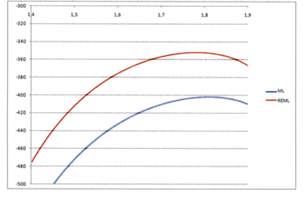
As explained in Section 4, the parameters for the ML models (Models II and III) are exactly the same. We also note that all the parameters of the REML model (Model IV) are very close to that of the ML models. For example, for p, Figure 1 illustrates the profile log-likelihood for the ML and REML models.

Figure 1.Penalized log-likelihood for varying p, for ML (Models II and III) and REML DGLM (Model IV)

It seems that the variance models indicate that the dispersion should be increasing as the development years mature. These results match perfectly the initial hypothesis described in Section 3. Moreover, the dispersion parameters are increasing monotonically, which indicates that there is no reversion in the severity trend: the more you wait, the bigger the variance of the outcome. Also, the change in dispersion from 240 to roughly 105,000 indicates that the slope of the overall trend is very steep, evidencing the force of the variance change that is required to calibrate the model to the data. We also note that only the first two columns have a dispersion smaller than the constant dispersion. All of the remaining columns have a dispersion parameter that is noticeably bigger.

5.4. Estimating the point reserve and the uncertainty level

The reserve point estimates and the mean squared error of prediction (MSEP) for all models are displayed in Table 6. First, all four models agree on similar reserve point estimates since the mean parameters were already very close. For all models, the MSEP was calculated using Formula (2.3). The covariance matrix we used is the inverse of the Fisher information matrix, which for Models III and IV is $\left(X^T W X\right)^{-1}$. Interestingly, the covariance matrix of the variance models is roughly four times that of Model I. Results of the MSEP in Table 7 show that dispersion modeling has a great impact on the estimation of the uncertainty of the reserve for this particular example.

In attempting to recognize that a constant dispersion with the likelihood principle was perhaps not enough, Wüthrich (2003) used an artificially estimated deviance-based dispersion parameter (with p fixed at 1.1741) that was 19 times bigger (Model V), where the parameter went from 1482 to 29,281. This Model V uses exactly the same parameters as Model I, but its dispersion parameter is estimated by the deviance principle. Table 7 illustrates the results. Still, it is unclear what methodology is best; we can just observe that the modeler’s decisions may impact the uncertainty level. Thus, in order to replicate exactly the model in Wüthrich (2003), the MSEP shown in Table 6 supposes that has been changed to 29,281. Yet, looking at the results, we do not see significantly different reserve uncertainty levels between Models II, III, and IV compared to Wüthrich’s model, at least on the aggregate accident year basis. There might be greater differences on a cell-by-cell basis because Models II, III, and IV allow for more flexibility.

5.5. Further discussion

It is important to note that allowing for a flexible variance structure does not guarantee that the overall variance in the model will be different, nor any of the reserve uncertainty levels per accident year. However, it is strongly suggested that variance modeling be considered when the modeler has reasons to believe that the underlying tendency of the frequency is different from the tendency of the severity. These tendencies can usually be uncovered by a direct one-way analysis. However, once the model is set up, the authors recommend an analysis of the pattern of the variance parameters in order to determine if a flexible variance structure is reasonable or not.

Note that Model IV (REML) produces generally somewhat lower estimates than Models II and III for this particular example. This seems contrary to the fact that REML tends to correct the ML tendency to underestimate dispersion. It turns out that Model IV has also different mean estimates which slightly alter the variance parameters. Had the mean parameters been the same, then the variance parameters would have been higher with the REML procedure. Thus, it should be noted that the REML procedure might prove useful as it corrects both the mean parameters (slightly) and the variance parameters.

Unfortunately, the REML procedure is not readily available in a direct maximum likelihood optimization. Recall that the REML scoring iteration (4.4) approximately maximizes with respect to γ the penalized log-likelihood:

$$l^{*}(y, \beta, \gamma, p)=l(y, \beta, \gamma, p)+\frac{1}{2} \log \left|X^{T} W X\right|$$

One can see that the determinant $\left|X^T W X\right|$ must be calculated for each iteration of the likelihood, and sadly, that cannot be done handily with standard statistical packages.

The small number of observations relative to the number of parameters gives rise to many practical problems for dispersion modeling. A problem of concern is the relatively large difference between the dispersion parameter of Model I, depending on the evaluation principle. In an attempt to better explain this phenomenon, Ruoyan (2004) presents an analysis on the micro-level of the calculation of the dispersion. Following his results, it turns out that the dispersion parameter estimated by the deviance principle (which is based on the observed total costs) is more sensitive to extreme values than if it was estimated by the likelihood principle. Since the number of observations in a claims reserving is usually low, the presence of only few extreme observations can distort the variance of the model. On the other hand, the likelihood estimator’s main contribution to the dispersion comes from the underlying frequency, which might be more stable than the total costs.

The model error associated with the choice of p is not considered here. One can refer to Peters, Shevchenko, and Wüthrich (2009) for a discussion on model error about the Tweedie model. It is well known that p is uncorrelated with the mean parameters (Smyth and Jørgensen 2002) and hence, it is not likely to influence the reserve point estimates too much. However, the variance might be affected as p and are very dependent. Standard errors for γ for estimation of p can be adjusted as done in Jørgensen and De Souza (1994).

Still, it is unclear whether p has the same effect on the variance parameters in a flexible variance structure as opposed to a constant one. One might argue that p could be interpreted as a competitor to the variance parameters, and thus its contribution to the model might be marginally lower as the number of variance parameters increase.

6. Conclusion

It has been shown that there exist situations in claims reserving where the variance needs to be modeled. We establish a flexible variance structure through direct maximum likelihood estimation and through double generalized linear models. We also use a restricted maximum likelihood as a correction to the variance parameters in the double generalized linear models. Having a flexible variance structure allows the model to replicate the underlying risk more appropriately and shrinks the gap between the predicted variances of different models.

Acknowledgments

Jean-Philippe Boucher would like to acknowledge the financial support from the Natural Sciences and Engineering Research Council of Canada.

Danaïl Davidov would like to thank the Université du Québec à Montréal for its financial support.