1. Introduction

Natural catastrophe reinsurance plays a vital role in the financial system by enabling homeowners, insurance companies, and governments to manage the negative consequences of large losses from hurricanes, earthquakes, severe storms, and inland and coastal flood events. One of the most common and important examples of natural catastrophe reinsurance is the catastrophe excess of loss (catXL) contract. CatXL contracts are typically purchased by primary insurance companies from reinsurers. CatXL coverage enables primary insurers to improve their risk/return profiles and remain solvent after the occurrence of severe natural catastrophes. Technical pricing of catXL reinsurance is fundamental to the workings of the insurance value chain. In nearly all cases, technical prices are derived from natural catastrophe simulation models using proprietary software, models, and data. Over the past two decades, significant resources have been devoted to the development of complex natural catastrophe risk models based in physics, statistics, and engineering. This reflects both the materiality of the risks involved and their complex nature.

The process of generating a technical price for a given catXL contract is best understood by example. Consider a primary insurance company whose portfolio of residential properties is scattered throughout the southeastern United States. We first create a database which stores all the relevant information about the buildings that compose the portfolio. A catastrophe modelling software is then run to generate a so-called timeline simulation of losses (accounting for limits and deductibles in the underlying homeowner policies) arising from various natural perils (e.g., hurricanes and severe convective storms). The timeline simulation of losses is then used as the basis for generating a technical price for a catXL reinsurance contract under various terms and conditions. Typically a large number of “simulation years” is used to avoid convergence errors (it is not uncommon to use 1 million years of simulation). In this work, we make a mathematical abstraction where we view the timeline simulation for a specific portfolio as being generated from a frequency distribution $P_{N}(k)$ (which describes the random number $N$ of events per year) and a severity distribution $f_{X}(x)$ (which describes the random financial loss $X$ in dollars given an event occurrence).

In this paper we look at the timeline simulations from the perspective of the so-called order statistics. Each year of simulation has an annual maximum loss, a second annual maximum, and so on. These ordered annual maxima are what we refer to as the order statistics. Previous studies have addressed the importance of the various order statistics in analysis of technical pricing metrics for catXL contracts (Khare and Roy 2021). As discussed in Khare and Roy (2021), the exceedance probabilities of the order statistics for various loss thresholds are fundamental to understanding which ordered maxima make the largest contributions to pricing metrics. With this in mind, the objective of this work is to develop and demonstrate a framework to quantify the implications of changes to the underlying catastrophe models (expressed through changes in the frequency $P_{N}(k)$ and severity $f_{X}(x)$) for the exceedance probabilities of the order statistics in timeline simulations. We presume that changes to the underlying frequency and severity arise for a number of reasons, but the primary reason we have in mind is climate change. In other words, this paper builds a mathematical framework that can be used as the basis for understanding the implications of climate change for technical reinsurance pricing. Given the urgent need to address issues related to climate change and the central role that reinsurance plays in risk transfer, this paper addresses an issue of clear societal relevance. While the focus in this paper is on the fundamental and mathematical aspects of this problem, we also discuss how our results can be used by practitioners to address the impacts of model changes arising from climate change on reinsurance pricing.

The mathematical problem of interest in this work is the order statistics of samples from a continuous distribution $f_{X}(x)$, with random sample sizes drawn from a discrete distribution $P_{N}(k)$. A series of papers addressing the order statistics under random sample sizes dates back to the 1970s (e.g., Barakat and El-Shandidy 2004; Buhrman 1973; Consul 1984; David and Nagaraja 2003; Gupta and Gupta 1984; Young 1970). Recently Khare and Roy (2021) discussed the order statistics problem within the context of reinsurance pricing, providing analytical expressions for the cumulative probability of all order statistics, the application to the commonly used Poisson and negative binomial distributions, as well as an analysis of the correlation structure of the order statistics. This paper builds on Khare and Roy (2021) by formalizing the presentation of the general formula for the cumulative probability of all order statistics, also casting the general formula into a form that is more useful from a practitioner’s point of view, and it explores the application of the general formula to a broader set of frequency distributions (including the binomial, the Generalized Poisson, and the Conway-Maxwell-Poisson). We use the mathematical machinery discussed in this paper to numerically demonstrate the sensitivity of the order statistic exceedance probabilities to changing model assumptions, achieving our main objective of building a framework which can aid in understanding the effect of climate change on reinsurance pricing metrics.

More specifically, the key contributions of this paper are as follows:

• We review the key result, which is the general expression of all order statistic cumulative probability distributions for a given frequency $P_{N}(k)$ and severity $f_{X}(x)$ (Theorem 3.2). The main result is equivalent to equation 9 in Khare and Roy (2021), but we provide a more clear, concise, and formal proof.

• We show that the main result, Theorem 3.2, can be reformulated in a form that is particularly appropriate for risk modelling, as it references explicitly the commonly discussed distribution of the annual maximum. The reformulated but mathematically equivalent result is provided in Corollary 3.3.

• We apply the general formulation in Corollary 3.3 to what we call the canonical frequency (consisting of the negative binomial, Poisson, and binomial distributions) to develop closed form expressions for the order statistic cumulative probability distributions. The results for the Poisson and negative binomial distributions are equivalent to those found in Khare and Roy (2021) but are reformulated into a simpler and more useful form. The result for the binomial distribution is new, as far as we know. The result is provided in Proposition 3.4.

• We provide a novel set of numerical experiments in which we apply the result from Corollary 3.3 to two commonly applied generalized frequency distributions, the Generalized Poisson (Consul and Jain 1973) and Cromwell-Maxwell-Poisson (Conway and Maxwell 1962). Our results suggest that the order statistics implied by the Generalized Poisson and Cromwell-Maxwell-Poisson are nearly identical to the canonical case. This is useful background knowledge in circumstances where the Generalized Poisson and/or Cromwell-Maxwell-Poisson distributions are applied (the generalized distributions have particular advantages discussed in Consul and Famoye 1990 and Sellers and Shmueli 2010).

• To address our central goal of understanding the implications of model changes to reinsurance pricing metrics, we provide a comprehensive investigation into how order statistic exceedance probabilities change as a function of altered frequency model assumptions. We achieve this by plotting what we call “Sensitivity Spaces” using the analytical formulas for the canonical case (Proposition 3.4). A number of new insights are achieved through our visualizations. Incidentally, our Sensitivity Space plots also shed light on a potential benefit of using one of the generalized frequency distributions rather than the canonical distribution (when the so-called frequency distribution dispersion is less than $1$).

• Finally, we tie together our mathematical and numerical work by discussing how practitioners can leverage our results to understand the potential impacts of climate change on reinsurance pricing metrics.

This paper is organized as follows. In Section 2 we discuss preliminaries, where we make clear various mathematical definitions, including the order statistic random variable, our notation, and various assumptions. In Section 3 we provide the analytical formulations of the order statistic distributions for a generic frequency $P_{N}(k)$ and severity $f_{X}(x)$, as well as closed form solutions for the canonical frequency (negative binomial, Poisson, and binomial). In Section 4 we discuss our numerical experiments and their implications. In Section 5 we discuss how practitioners can use the results in this paper to understand the implications of climate change for reinsurance pricing metrics. Section 6 provides a summary, draws conclusions, and discusses future research directions.

2. Preliminaries

The risk models central to this work consist of a discrete frequency distribution and a continuous severity distribution to generate so-called timeline simulations of event and loss occurrences that form the basis for risk quantification. We start here with preliminaries to make clear various mathematical definitions, the problem statement, and our intended application to risk modelling. Some elementary definitions are provided for completeness and context. We start with the discrete frequency distribution.

Definition 2.1. Frequency distribution: The random number of events over a specified time interval (taken to be 1 year without loss of generality) is given by $N$ and has a discrete frequency distribution $P_{N}(k)$, where $k\in[0,1,2,..,\infty)$, and $\sum_{k=0}^{\infty}P_{N}(k)=1$.

The expectation and variance of the frequency distribution are denoted by $\mathbb{E}\left[N\right]$ and $\mathbb{V}\left[N\right]$ respectively, and their ratio is the well-known dispersion parameter defined as follows.

Definition 2.2. Dispersion: The dispersion of a frequency distribution is

$$D=\frac{\mathbb{V}\left[N\right]}{\mathbb{E}\left[N\right]},$$

where $D\in(0,\infty).$

One of the main goals of this work is to explore the sensitivity of practically important risk model metrics to the expectation ($\mathbb{E}\left[N\right]$) and variance ($\mathbb{V}\left[N\right]$) over the full range of dispersion $D\in(0,\infty)$. To enable this, we define what we call the canonical frequency distribution, consisting of the triad of frequency distributions given by the negative binomial for $D>1$, the Poisson for $D=1$, and the binomial for $D\in(0,1)$. We label this combination of frequency distributions as the canonical case due to its common application in risk modelling and various well-known mathematical properties (Klugman, Panjer, and Willmot 2008).

Definition 2.3. Canonical frequency distribution: For $D>1$, $P_{N}(k)$ is given by the negative binomial distribution,

$$P_{N}(k)=\frac{\Gamma(k+r)}{k!\Gamma(r)}p^{r}(1-p)^{k},\tag{2.1}$$

where $r=\frac{\mu^{2}}{\sigma^{2}-\mu}>0,$ $\Gamma(r)$ is the gamma function $\Gamma(r)=\int_{0}^{\infty}s^{r-1}e^{-s}ds$ (for $r>0$), $p=\frac{\mu}{\sigma^{2}}$, $\mathbb{E}\left[N\right]=\mu$, $\mathbb{V}\left[N\right]=\sigma^{2}$, and $p\in(0,1)$ (which confirms $D>1$, and note that $r=\frac{\mu}{D-1}$).

For $D=1$, $P_{N}(k)$ is given by the Poisson distribution,

$$P_{N}(k)=\frac{e^{-\lambda}\lambda^{k}}{k!},\tag{2.2}$$

where $\lambda$ is a positive real number with $\mathbb{E}\left[N\right]=\mathbb{V}\left[N\right]=\lambda$ (which confirms $D=1$).

For $D\in(0,1)$, $P_{N}(k)$ is given by the binomial distribution,

$$P_{N}(k)=\left(\begin{array}{c} n\\ k \end{array}\right)q^{k}(1-q)^{n-k},\tag{2.3}$$

where $\mathbb{E}\left[N\right]=nq$, $\mathbb{V}\left[N\right]=nq(1-q)$, $n$ is a positive integer such that $n\geq k$, and $q\in(0,1)$ (which confirms $D=(1-q)\in(0,1)$). For the binomial distribution we note that $\sum_{k=0}^{n}\left(\begin{array}{c} n\\ k \end{array}\right)q^{k}(1-q)^{n-k}=1$, and for $k>n$ the factorial term is defined to be $0$, and hence $P_{N}(k)=0$.

The canonical frequency distribution defined above unifies the commonly applied and well-understood negative binomial, Poisson, and binomial cases. In practical applications, the canonical frequency distribution is not without issues. For dispersion $D\in(0,1)$ (binomial), we are restricted to positive integer values of $n$, which implies that for (empirical) target values of $\mathbb{E}\left[N\right]$ and $\mathbb{V}\left[N\right]$, some approximation may be required due to rounding of $n$. Secondly, in a regression context, other more general frequency distributions that cover the full range of $D\in(0,\infty)$ in one expression for $P_{N}(k)$ have certain advantages (Consul and Famoye 1990; Sellers and Shmueli 2010). In this work, to compare and contrast with the canonical case, we study two commonly applied generalized frequency distributions. Following Consul and Jain (1973) and Scollnik (1998), we define the Generalized Poisson as follows.

Definition 2.4. Generalized Poisson distribution: For dispersion values $D\in[1,\infty)$, the Generalized Poisson is given by

$$P_{N}(k)=\frac{\alpha(\alpha+k\beta)^{k-1}e^{-(\alpha+k\beta)}}{k!},\tag{2.4}$$

where $\alpha>0$, $\beta\in[0,1)$, $\mathbb{E}\left[N\right]=\frac{\alpha}{(1-\beta)}$, $\mathbb{V}\left[N\right]=\frac{\alpha}{(1-\beta)^{3}}$, and $D=\frac{1}{(1-\beta)^{2}}\in[1,\infty)$. We note that when $\beta=0$ the Generalized Poisson is equivalent to the Poisson distribution.

For the under-dispersive case where $D\in(0,1)$, with $\alpha>0$, $\beta<0$, we must generally include a normalization factor $C(\alpha,\beta)$, such that

$$P_{N}(k)=\frac{\alpha(\alpha+k\beta)^{k-1}e^{-(\alpha+k\beta)}}{k!C(\alpha,\beta)},(k)=0,\tag{2.5}$$

and

$$P_{N}(k)=0$$

for

$$k\geq m,$$

where $m$ is the smallest positive integer value that satisfies

$$\alpha+m\beta\leq0.$$

We are not aware of closed form solutions for $\mathbb{E}\left[N\right]$, $\mathbb{V}\left[N\right]$, or $C(\alpha,\beta)$ when $\beta<0$, but these are readily computed (only finite sums are required due to truncation). Our definition follows Scollnik (1998), which discusses and rectifies some of the issues discussed in the original formulation (Consul and Jain 1973)—in particular for the under-dispersive $\beta<0$ case, where one can easily construct cases that prove a normalization factor is required, and that the analytical forms for $\mathbb{E}\left[N\right]$ and $\mathbb{V}\left[N\right]$ when $\beta\in[0,1)$ do not hold when $\beta<0$.

The Generalized Poisson enables one to cover the full range of dispersion values $D\in(0,\infty)$ and in some sense does so in a “smooth” manner, as the analytical form for $P_{N}(k)$ is fixed (aside from the normalization factor required when $\beta<0$). Another generalized frequency distribution is the Cromwell-Maxwell-Poisson (CMP) distribution that has been used in risk analysis (Guikema and Coffelt 2008). Following Conway and Maxwell (1962) we now provide the definition.

Definition 2.5. Cromwell-Maxwell-Poisson frequency distribution: The CMP distribution is given by

$$P_{N}(k)=\frac{\gamma^{k}}{(k!)^{\nu}Z(\gamma,\nu)},\tag{2.6}$$

where $Z(\gamma,\nu)=\sum_{j=0}^{\infty}\frac{\gamma^{j}}{(j!)^{\nu}}$, $\gamma>0$, and $\nu\geq0$. We note that $\mathbb{E}\left[N\right]=\sum_{l=0}^{\infty}\frac{l\gamma^{l}}{(\gamma!)^{\nu}Z(\gamma,\nu)}$, and $\mathbb{V}\left[N\right]=\sum_{l=0}^{\infty}\frac{l^{2}\gamma^{l}}{(\gamma!)^{\nu}Z(\gamma,\nu)}-\left(\mathbb{E}\left[N\right]\right)^{2}$. $D\in(0,1)$ when $\nu>1$, $D=1$ (Poisson) when $\nu=1$, and for $D>1$ we must have $\nu\in(0,1)$ (note that $\nu=0$ requires $\gamma\in(0,1)$).

Much like the Generalized Poisson, the CMP distribution enables us to model the full range of dispersion values ($D\in(0,\infty)$) without requiring a change in the analytical form. Taking stock, all three distributions defined so far describe the random number of so-called event occurrences within a year. To complete the picture for the risk model, we assign a financial loss to each event occurrence. For this we use a severity distribution defined as follows.

Definition 2.6. Severity distribution: The continuous severity distribution, written as a density, is given by

$$f_{X}(x),$$

where the financial loss for a specific portfolio of assets is $x\in[0,\infty)$ (and so $\int_{0}^{\infty}f_{X}(x)dx=1$).

Definition 2.7. Hereafter we use the convenient shorthand $f$ to denote the cumulative probability at a given loss threshold $l\in[0,\infty)$ where

$$f\equiv\int_{0}^{l}f_{X}(x)dx.$$

Having established the definitions for the frequency and severity distributions, we impose the assumption that samples from $P_{N}(k)$ and $f_{X}(x)$ are drawn independently (often assumed in insurance applications, but see Shi, Feng, and Ivantsova [2015] to explore relaxing this assumption). The combination of the frequency $P_{N}(k)$ and severity $f_{X}(x)$ represents a mathematical abstraction of a risk model applied to a specific portfolio of assets. For example, this may represent the application of a hurricane catastrophe model to a primary insurance portfolio. While a complex bottom-up process is required to build a useful hurricane catastrophe model, our top-down abstraction enables us to assess the impact of alternative (high-level) model assumptions on important loss metrics in a straightforward way.

The practical application of risk modelling typically makes use of what we call timeline simulation. Timeline simulation involves sampling both $P_{N}(k)$ and $f_{X}(x)$ in a sequence that generates losses for a specified set of simulation years. One advantage of timeline simulation is the ability to apply complex financial contracts. A formal definition makes the notion of timeline simulation clear.

Definition 2.8. Timeline simulation: A timeline simulation for $S$ years is defined by the following process:

1. For all years indexed by $i=1,...,S$,

2. draw a random number from the frequency distribution $P_{N}(k)$;

3. for each year $i$ let the random realization be $N=k_{i}$, which implies that we must take $k_{i}$ random (loss) samples from the severity $f_{X}(x)$ (all samples are tagged with year $i$).

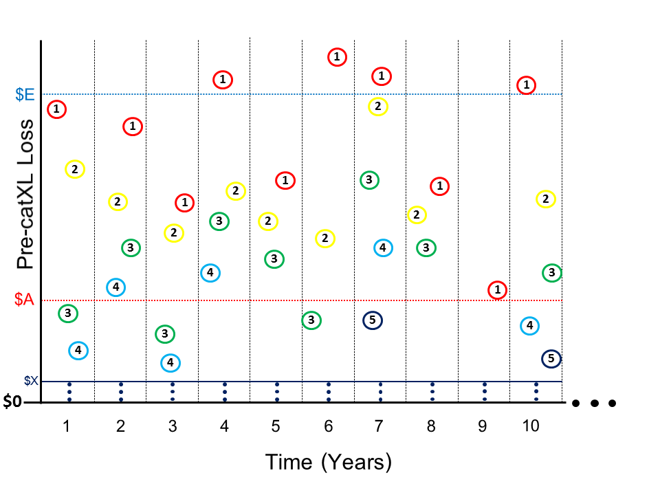
To better understand Definition 2.8, we provide a visualization in Figure 1.

Figure 1.A depiction of a timeline simulation for a given frequency $P_N(k)$ and severity $f_X(x)$.

Each simulation period is one-year in length (x-axis). The y-axis is the primary insurer portfolio loss in $, before the application of any reinsurance. The annual maximum loss events are depicted by the 1’s with red circles. Second annual maximum losses are indicated by the 2’s with yellow circles and so on. Event losses that are less than or equal to $X < $A have values in the closed interval from $0 to $X. The dashed red and blue lines indicated by the $A and $E values correspond to the attachment and exhaustion point of a catXL reinsurance contract that will be applied in what follows.

Figure 1 depicts a timeline simulation generated from a given $P_{N}(k)$ and $f_{X}(x)$. The y-axis represents loss to a primary insurer before the application of reinsurance (and “Pre-catXL” makes clear the losses are depicted before the application of a catXL contract). In Figure 1, the catXL contract is represented by the attachment point $A and exhaustion point $E. Depending on the type of catXL contract, losses within this layer are the responsibility of the reinsurer (see Mata [2000], Khare and Roy [2021], and Cummins, Lewis, and Phillips [1991] for formal mathematical definitions). Figure 1 visualizes the order statistics that are central to this study. The 1s in red circles depict the annual maxima, the 2s in yellow circles depict the second annual maxima, and so on. We use the following notation for the order statistics.

Definition 2.9. We adopt the classical compound claims notation (Klugman, Panjer, and Willmot 2008) with a slight modification to meet our needs. Suppose that, for a given year of timeline simulation using $P_{N}(k)$ and $f_{X}(x)$, the number of events $N=k$. For this particular year, we take $N=k$ random draws from $f_{X}(x)$ and order them in the following way:

$$\begin{align} (X_{1}=x_{1})&\geq(X_{2}=x_{2})\geq...\geq(X_{k}=x_{k})\\ &\geq(X_{k+1}=0)=...=(X_{\infty}=0). \end{align}$$

Note that we assign the value of $0$ to all order statistics labelled by $k+1$ and above. This deviates from our interpretation of the classical compound claims notation in that we formally recognize the losses indexed by $k+1$ and above (which are assigned a value of $0$). Note that $X_{1}=x_{1}$ is the realized value of the annual maximum (recall we are using one-year time periods), $X_{2}=x_{2}$ is the realized value of the second maximum, and so on. This labelling of the order statistics also deviates from convention in that $X_{1}$ is typically labelled the smallest loss (David and Nagaraja 2003). Our notation suits our study where there is not a fixed number of events in a given year, and is perhaps more intuitive in that the subscript 1 is used to indicate the maximum (an ordinal ranking).

With our notation in hand, we now provide the mathematical definition of the order statistics.

Definition 2.10. For a given $P_{N}(k)$ and severity $f_{X}(x)$, the $M$th order statistic random variable is $X_{M}$, where $X_{1}\geq X_{2}\geq X_{3}\geq...$, and the integer index $M\in[1,2,3,...,\infty)$.

We have set the stage for the next section, where we provide the mathematical formulation of the order statistic distributions.

3. Order statistics in frequency and severity modelling

With Figure 1, Definition 2.10, and Notation 2.9 in hand, our goal is to formulate the cumulative probability of the random variable $X_{M}$ for some loss threshold $l\in[0,\infty)$ and integer $M\in[1,2,3,...,\infty)$. We first show the general formula for a generic discrete frequency distribution, and later apply the formula to the canonical case where closed form solutions are achieved. We also discuss the application to the Generalized Poisson and CMP distributions. We start with the definition of the order statistic cumulative probability.

Definition 3.1. Order statistic cumulative probability: The order statistic cumulative probability $F_{X_{M}}(l)$ is

$$F_{X_{M}}(l)=\sum_{k=0}^{\infty}P_{N}(k)F_{X_{M}}(l\mid N=k),$$

where $F_{X_{M}}(l\mid N=k)$ is the cumulative probability of the $M$th order statistic random variable, up to loss threshold $l$, given $N=k$ events, with $M\in[1,2,3,...,\infty)$.

The definition of the order statistic cumulative probability involves both frequency and severity. The frequency term $P_{N}(k)$ accounts for the probabilities associated with different realizations of the number of events (in a one-year time period). The cumulative probability term $F_{X_{M}}(l\mid N=k)$ is conditional on the ordering/configuration of the $N=k$ events about the loss threshold $l$ (hence the conditional notation). It is clear that when the number of events is less than the order (i.e., $k<M$), it must be that $X_{M}=0$ (following Definition 2.10 using Notation 2.9). Hence, when $k<M$, $F_{X_{M}}(l|N=k)=1$ for all $l\in[0,\infty)$. The terms in Definition 2.11 where $k\geq M$ require some careful argumentation that leads to the following key result stated as a theorem.

Theorem 3.2. Order statistic cumulative distribution: The order statistic cumulative probability $F_{X_{M}}(l)$ up to loss threshold $l$ is given by

$$\begin{align} F_{X_{M}}(l)&=\sum_{k=0}^{M-1}P_{N}(k)\\ &\quad+\sum_{k=M}^{\infty}P_{N}(k)\sum_{i=0}^{M-1}\left(\begin{array}{c} k\\ i \end{array}\right)(1-f)^{i}f{}^{k-i}, \end{align} \tag{3.1}$$

where $X_{M}$ is the $M$th order statistic random variable, $P_{N}(k)$ is the frequency distribution, the severity $f=\int_{0}^{l}f_{X}(x)dx$ (for loss threshold $l$), and $M\in[1,2,3,...,\infty)$. A proof is provided in Appendix A.

We note that $1-F_{X_{1}}(l)\equiv OEP(l)$, where the notation $OEP$ commonly stands for the “occurrence exceedance probability.” In reinsurance applications, the $OEP(l)$ is one of the most important distributions, as it is associated with the annual maximum ($M=1$), which in many cases explains a large proportion of reinsurance pricing metrics (Khare and Roy 2021). With the importance of the $OEP(l)$ in mind, we are motivated to reformulate Equation (3.1) in a way that makes explicit reference to the $F_{X_{1}}(l)$ function. Doing so will enable insight as to how the higher orders amplify (or add to) the $F_{X_{1}}(l)$. We first note that, using Equation (3.1) for $M=1$, we obtain

$$F_{X_{1}}(l)=\sum_{k=0}^{\infty}P_{N}(k)f{}^{k}.\tag{3.2}$$

The above formula is the probability generating function of $f$ (the formula is intuitive in that when $N=k$ we require all events to be below $l$, which has probability $f^{k}$). The following corollary demonstrates how we can rewrite Equation (3.1) making explicit reference to $F_{X_{1}}(l)$.

Corollary 3.3. Alternative formulation of the $F_{X_{1}}(l)$ general formula for $M\geq2$: The $M$th order order statistic cumulative probability can be written as follows:

$$\begin{align} F_{X_{M}}(l)&=F_{X_{1}}(l)\\ &\quad+\sum_{i=1}^{M-1}\sum_{k=i}^{\infty}P_{N}(k)\left(\begin{array}{c} k\\ i \end{array}\right)(1-f)^{i}f^{k-i}, \end{align} \tag{3.3}$$

for $M\geq2$. A proof is provided in Appendix B.

We now discuss the application of Equation (3.3) from Corollary 3.3 to the canonical frequency distributions, where we are able to obtain closed form solutions. Our aim is to write the $F_{X_{M}}(l)$ expressions as functions of $D,\mathbb{E}\left[N\right]$, and $f$. This formulation is helpful as we later explore the values of these functions in $D,\mathbb{E}\left[N\right]$ space (for various fixed loss thresholds $l$ and therefore $f$) as a way of understanding sensitivity of the order statistic distributions to model assumptions. The result for the canonical case is stated as a proposition.

Proposition 3.4. The canonical $F_{X_{M}}(l)$ distribution for $M\geq2$: For dispersion $D\in(1,\infty)$, the canonical frequency distribution is the negative binomial, for which the $F_{X_{M}}(l)$ function is

$$\scriptsize{ \begin{align} &F_{X_{M},}{}_{nb}(l)\\ &\quad =F_{X_{1},}{}_{nb}(l)\left(1+\sum_{i=1}^{M-1}\frac{\Gamma\left(i+\frac{\mathbb{E}\left[N\right]}{D-1}\right)}{\Gamma\left(\frac{\mathbb{E}\left[N\right]}{D-1}\right)i!}\left(\frac{D(1-f)+f-1}{D(1-f)+f}\right)^{i}\right), \end{align} \tag{3.4} }$$

where $F_{X_{1},}{}_{nb}(l)=\left(D(1-f)+f\right)^{\frac{\mathbb{E}\left[N\right]}{1-D}}$, $\mathbb{E}\left[N\right]=\mu$ ($\mu$ from Definition 2.3), and $f=\int_{0}^{l}f_{X}(x)dx$.

For $D=1$, the canonical frequency distribution is the Poisson, for which the $F_{X_{M}}(l)$ function is given by

$$\small{ \begin{align} F_{X_{M},}{}_{pois}(l)=F_{X_{1},}{}_{pois}(l)\left(1+\sum_{i=1}^{M-1}\frac{\left(\mathbb{E}\left[N\right](1-f)\right)^{i}}{i!}\right), \end{align} \tag{3.5} }$$

where $F_{X_{1},pois}(l)=e^{-\mathbb{E}\left[N\right](1-f)}$, $\mathbb{E}\left[N\right]=\mathbb{V}\left[N\right]=\lambda$ ($\lambda$ from Definition 2.3), and $f=\int_{0}^{l}f_{X}(x)dx$ (note that $\mathbb{E}\left[N\right](1-f)=\lambda(1-f)$ is what we refer to as the “Event Exceedance Frequency” or $EEF(l)$, commonly discussed in the risk modelling community).

For $D\in(0,1)$, the canonical frequency distribution is the binomial, for which the $F_{X_{M}}(l)$ function is given by

$$\scriptsize{ F_{X_{M},}{}_{bn}(l)=F_{X_{M},}{}_{bn}(l)\left(1+\sum_{i=1}^{M-1}\left(\begin{array}{c} \frac{\mathbb{E}\left[N\right]}{1-D}\\ i \end{array}\right)\left(\frac{(1-f)(1-D)}{D+(1-D)f}\right)^{i}\right),\tag{3.6} }$$

where $F_{X_{1},}{}_{bn}(l)=(D+(1-D)f)^{\frac{\mathbb{E}\left[N\right]}{1-D}}$, $\mathbb{E}\left[N\right]=nq,$ $\mathbb{V}\left[N\right]=nq(1-q)$, $D=(1-q)$, $q\in(0,1)$, $n\in[1,2,3,...,\infty]$, and $f=\int_{0}^{l}f_{X}(x)dx$ (note that $\frac{\mathbb{E}\left[N\right]}{1-D}$ is an integer and $\left(\begin{array}{c} \frac{\mathbb{E}\left[N\right]}{1-D}\\ i \end{array}\right)$ evaluates to $0$ when $i>\frac{\mathbb{E}\left[N\right]}{1-D}$).

Proofs of Equations (3.4, 3.5, 3.6) are provided in Appendix C, D, and E respectively.

Proposition 3.4 provides the $F_{X_{M}}(l)$ functions for the canonical frequency and enables us to model cases which cover the full range dispersion values $D\in(0,\infty)$. The three functions $F_{X_{M},}{}_{nb}(l)$, $F_{X_{M},pois}(l)$, and $F_{X_{M},bn}(l)$ are interesting in that the higher order terms ($M\geq2$) are achieved by multiplying the “base” $M=1$ function associated with the annual maximum ($F_{X_{1}}(l)$) by the terms in the brackets, which amplify the base annual maximum function. It is clear that the amplification factors grow with the order $M$ (since all terms in the brackets are positive numbers), as we would expect given the ordering inherent to the order statistic random variables. Finally, we note that, as the order $M$ increases, the amplification factor must converge since the cumulative probability has an upper bound of $1$. This can be seen formally by taking a limit as $M\rightarrow\infty$ (omitted for brevity). For the binomial case ($D\in(0,1)$) this is immediately clear since the factorial term $\left(\begin{array}{c} \frac{\mathbb{E}\left[N\right]}{1-D}\\ i \end{array}\right)$ evaluates to $0$ when $i>\frac{\mathbb{E}\left[N\right]}{1-D}$ (so higher orders do not contribute to amplification of the base annual maximum cumulative probability). In the case of the Poisson and negative binomial, all orders $M$ contribute to the amplification factor (although marginally for larger $M$), contrasting with the binomial case where at some point the contribution of the higher orders to the amplification factor is nil.

We have also explored the application of Corollary 3.3 to the generalized frequency distributions discussed above. For the Generalized Poisson case, as far as we are aware, there is no closed form solution where we can eliminate the infinite sum. The CMP is even more challenging as there is no closed form solution for the distribution itself. In what follows, we use numerical approximations when applying Corollary 3.3 to the Generalized Poisson and CMP distributions (where the main considerations are computational complexity and accuracy).

With the above analytical formulations in hand, we proceed with numerical experimentation in the next section.

4. Numerical experiments

Here we provide a brief set of numerical results with two objectives in mind. Our first objective is to visualize the order statistic distributions for the canonical case, make some qualitative observations as to how the distributions change as a function of $\mathbb{E}[N]$ and $D$, and make comparisons with results generated from the Generalized Poisson and CMP distributions for specific cases. Secondly, we demonstrate what we call Sensitivity Spaces where, using analytical equations for the canonical case, we visualize the order statistic exceedance probability distributions as a function of $\mathbb{E}[N],D$ for a variety of orders $M$ and fixed values of $f$ (and implicitly loss thresholds $l$). The Sensitivity Space analysis for the canonical case enables us to quickly understand the degree to which important loss metrics change as a function of altered frequency model assumptions (this has relevance for understanding changes to reinsurance attachment probabilities under changing climates). Our Sensitivity Space analysis also enables us to make clear a potential advantage of using one of the generalized frequency distributions compared with the canonical frequency.

4.1. Comparison of the canonical and generalized frequency distribution order statistic distributions

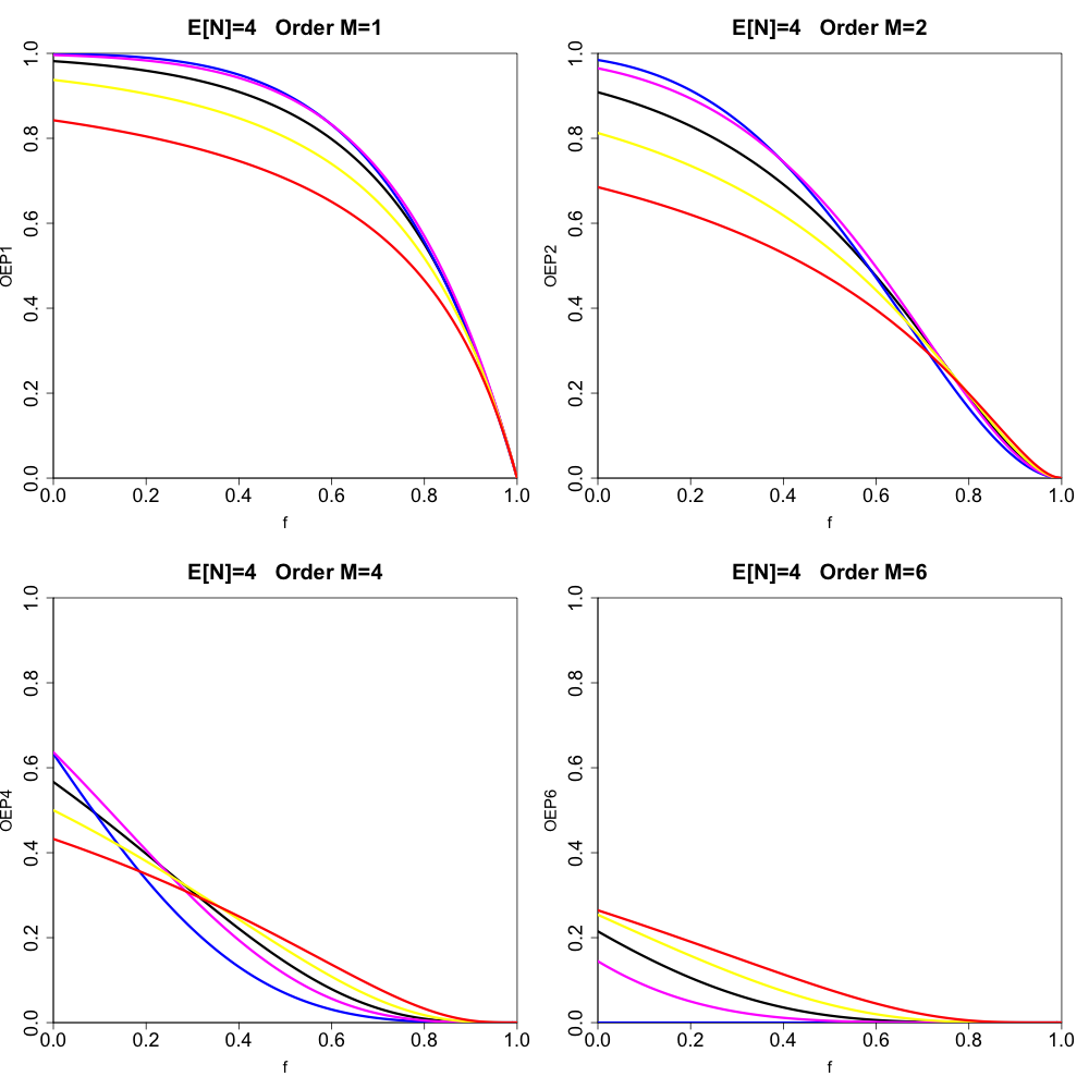
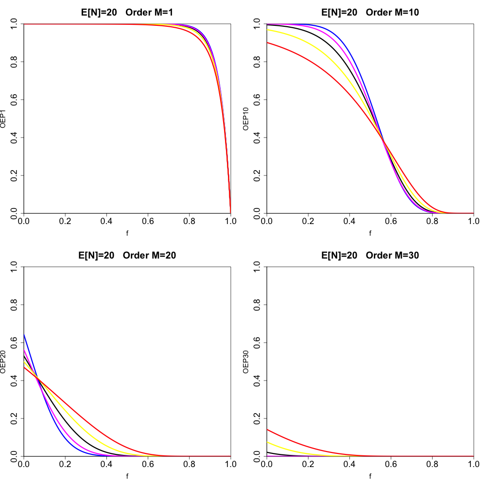
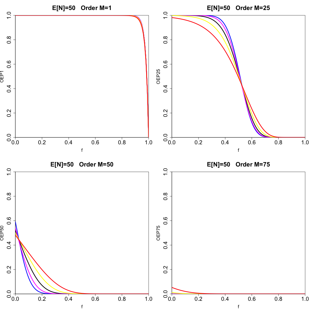
We start by simply displaying the canonical order statistic exceedance probabilities for a variety of cases (using Proposition 3.4). The upper-left panel of Figure 2 displays results for the case where $\mathbb{E}[N]=4$, with dispersion values $D=1$ (black), $D=4$ (red), $D=2$ (yellow), $D=0.5$ (magenta), and $D=0.25$ (blue) for order $M=1$. Exceedance probability ($1-F_{X_{1}}(l)$) is displayed on the y-axis, and $f=\int_{0}^{l}f_{X}(x)dx$ is displayed on the x-axis (ranging from $0$ to $1$ in increments of $0.01$). Higher orders are plotted on the upper-right, lower-left, and lower-right panels (chosen so that we display order $M=\mathbb{E}[N]/2$, $M=\mathbb{E}[N]$, and $M=3\mathbb{E}[N]/2$). In Figures 3 and 4 we show cases where $\mathbb{E}[N]=20$ and $\mathbb{E}[N]=50$ (and we have chosen the orders scaled to $\mathbb{E}[N]$ in the same way as in Figure 2). We note that, for the under-dispersive cases $D=0.5$ and $D=0.25$, we use the following convention to get the parameters $n$ and $q$ from Definition 2.3. We first obtain $q$ by solving the equation $D=(1-q)$. We then let $n=\lfloor\mathbb{E}[N]q\rfloor$ (the floor function), which introduces a slight (unavoidable) approximation. Now, looking at the combined results displayed in Figures 2, 3, and 4, we make some qualitative observations:

Figure 2.The upper left panel depicts the order $M=1$ order statistic exceedance probabilities, for $\mathbb{E}[N]=4$, with varying values of dispersion: $D=1$ (black), $D=4$ (red), $D=2$ (yellow), $D=0.5$ (magenta) and $D=0.25$ (blue). The upper right panel depicts the results for $M=2$, the lower left with $M=4$ and the lower right has $M=6$.

Figure 3.Results analogous to Figure 2 except that $\mathbb{E}[N]=20$ and for orders $M=[1,10,20,30]$.

Figure 4.Results analogous to Figure 2 except that $\mathbb{E}[N]=50$ and for orders $M=[1,25,50,75]$

The upper-left panel of Figure 2 demonstrates that, for the order $M=1$ distribution, over-dispersion $D\in(1,\infty)$ lowers the exceedance probability, whereas under-dispersion $D\in(0,1)$ increases the exceedance probability.

Again for the upper-left panel of Figure 2, we see that the two under-dispersive exceedance probability curves cross each other, unlike the over-dispersive case where the curves do not cross (which we have checked numerically).

For orders $1\leq M\leq\mathbb{E}[N]$, it appears that the over-/under-dispersive cases cross over with the Poisson $D=1$ case for some value of $f\in(0,1)$.

Looking at Figures 2, 3, and 4 as a whole, we see that, for a fixed value of $f$, changes in the value of the dispersion parameter have a more prominent effect on the variation in the various exceedance probabilities curves for smaller values of $\mathbb{E}[N]$. For example, the over-/under-dispersive cases are further apart in Figure 2 than in Figure 4.

We believe it is possible to formalize most of the above qualitative observations into precise mathematical statements. This is left to future work.

We now focus on two specific cases where we compare the order statistic distributions from the generalized frequency distributions to those obtained with the canonical frequency. A priori, we do not expect to see vast differences, as the frequency distributions can be shown to align (to a good approximation) with the canonical frequency distributions (Consul and Jain 1973). Still, we are motivated to investigate this given the advantages of the generalized frequency distributions discussed in the literature (Consul and Famoye 1990; Sellers and Shmueli 2010). We start with the Generalized Poisson distribution.

As discussed above, we do not have a closed form solution for the order statistic cumulative probability when we assume a Generalized Poisson, hence we resort to numerical calculation using the general formula given by Equation (3.1) from Theorem 3.2. In all instances when we use Equation (3.1), we truncate the infinite sum such that the maximum value of $k$ is $100$. We have found this to be an accurate value for the truncation (which we ascertained by computing the percentage difference to the case with maximum $k$ of $101$, deemed to be small enough; details are omitted for brevity). We have generated results for the over-dispersive case where $D=2$ and $\mathbb{E}\left[N\right]=10$, using the analytic formulas in Definition 2.4, yielding parameter values $\alpha=7.071068$ and $\beta=0.2928932$ (hereafter all such numbers are displayed with 8 significant digits). For the under-dispersive case with target dispersion $D=0.5$, we have done a numerical search over $\alpha$ and $\beta$ space, which yields parameter values $\alpha=14.140$ and $\beta=-0.414$, with $\mathbb{E}[N]=10.000007$ and $\mathbb{V}[N]=5.001442$, which implies $OD=0.5001438$. This was deemed sufficiently accurate to enable a valid comparison to the canonical case where $OD=0.5$. The results are displayed in Figure 5, whose presentation is analogous to Figure 2 but with the addition of the over- and under-dispersive Generalized Poisson cases indicated by the yellow and magenta circle markings. We see that for all orders $M=[1,5,10,15]$ there is very little difference between the canonical and Generalized Poisson results (despite the numerical approximation required for the under-dispersive case for both the canonical and Generalized Poisson). Our results hint at a general principle: the implied order statistic distributions from the Generalized Poisson closely approximate those obtained using the canonical frequency distribution. This is useful to know in contexts where the Generalized Poisson is applied.

Figure 5.Results analogous to Figure 2 except that $\mathbb{E}[N]=10$ and for orders $M=[1,5,10,20]$.

The yellow dots depict results derived from the Generalized Poisson distribution for $D=2$ (with parameter values $\alpha=7.071068$ and $\beta=$ 0.2928932 obtained using the exact formulas for the expectation and variance), and the magenta dots depict results from the Generalized Poisson for $D=0.5$ (with parameter values $\alpha=14.140$ and $\beta=-0.414$ obtained using a numerical scheme discussed in the main text).

Figure 6 displays results analogous to Figure 5, replacing the Generalized Poisson with the CMP distribution. Recall from Definition 3.4 that the CMP has no closed form solution for the frequency itself. To compute the frequency distribution values in Definition 2.5, we use maximum values of $j,l$ of $100$ in computing $Z(\gamma,\nu)$, $\mathbb{E}\left[N\right]$, and $\mathbb{V}\left[N\right]$ (we have tested accuracy by checking maximum values computed for $j,l$ of 100 and deemed the results to be accurate; details are omitted for brevity). We also use numerical calculation in our application of Equation (3.1) from Theorem 3.2 (using the same maximum value for $k$ of $100$ in the infinite sum, again found to have an accurate solution). To determine the values of the CMP model parameters that capture the target dispersion values of $D=2$ and $D=0.5$ (for $\mathbb{E}\left[N\right]=10$), we perform a search algorithm in $\gamma,\nu$ space. For the target $D=2$ case, we find that $\gamma=118.25$, $\nu=2.05$ gives $\mathbb{E}\left[N\right]=10.000061$, $\mathbb{V}[N]=5.001442$, and implied $D=0.5001438$. For the under-dispersive target dispersion $D=0.5$, we find that $\gamma=2.856$, $\nu=0.468$ gives $\mathbb{E}\left[N\right]=10.007889$, $\mathbb{V}[N]=20.04255$, and implied $D=2.002675$. These numerical results were deemed accurate enough for a valid comparison to the canonical case. The results in Figure 6 (with identical format to Figure 5) demonstrate that the CMP distribution also yields similar order statistic distributions across orders displayed in Figure 5. Our results for the CMP again hint at a general principle: that the generalized frequency distributions yield similar order statistic distributions.

Figure 6.Results analogous to Figure 2 with results from the Generalized Poisson replaced with the CMP.

The yellow dots depict results derived from the CMP distribution for $D=2$ (with parameter values $\gamma=2.856$ and $\nu=0.468$ obtained using the numerical scheme discussed in the main text), and the magenta dots depict results from the CMP for $D=0.5$ (with numerically derived parameter values of $\gamma=118.250$ and $\nu=2.05$ ).

4.2. Sensitivity of order statistic exceedance probabilities to canonical frequency model assumptions

Here we investigate how exceedance probabilities, for various fixed values of $f=\int_{0}^{l}f_{X}(x)dx$ (and implicitly loss thresholds), change as we vary $\mathbb{E}[N]$ and $\mathbb{V}[N]$ (and implicitly $D$). The visualizations to follow are what we call “Sensitivity Spaces.” Our over-arching motivation is to provide useful insight as to how key loss exceedance probability metrics change as model assumptions change. We generate results for the canonical frequency distribution only, taking advantage of the analytical solutions provided by Proposition 3.4, which enables us to plot the exceedance probabilities in $\mathbb{E}[N]$ and $D$ space at high resolution.

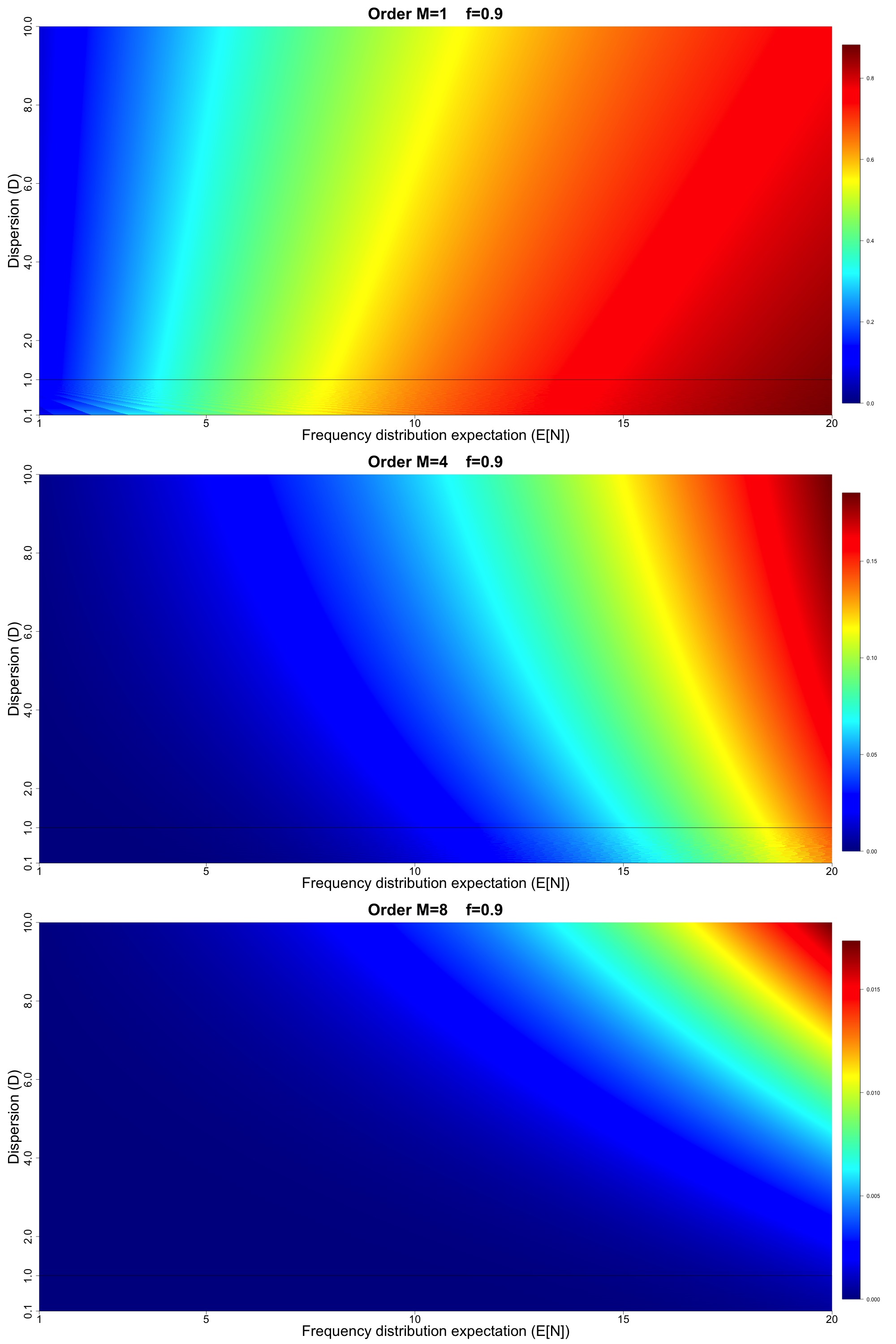
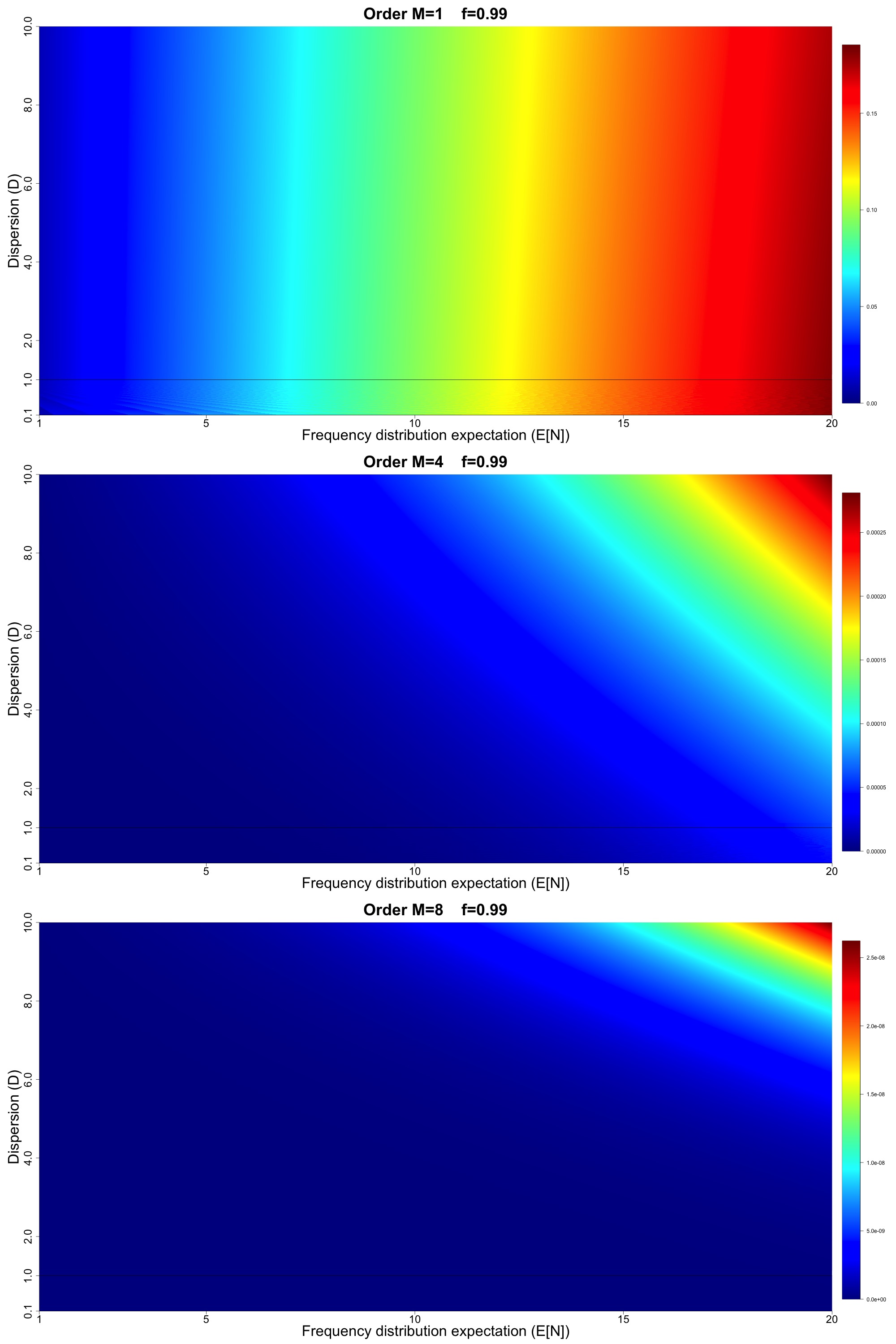
The upper panel of Figure 7 displays the order $M=1$ exceedance probability values for $f=0.5$. Figure 7 displays results for $D\in[0.1,10]$ in increments of $0.0025$, and $\mathbb{E}[N]\in[1,20]$ in increments of 0.0025 (for a total of over $29.5$ million model configurations). The middle panel of Figure 7 displays the analogous results for order $M=4$, and the lower panel displays results for order $M=8$. All panels in Figure 7 have a thin black horizontal line at $D=1$ to indicate the crossover point between under- and over-dispersive.

Figure 7.The upper panel displays the exceedance probabilities associated with the order $M=1$ order statistic distributions $\left(1-F_{X_1}(l)\right)$ for a variety of dispersion values $D \in[0.1,10]$ and frequency distribution expectations $\mathbb{E}[N] \in[1,20]$, with fixed severity loss threshold such that $f=0.5=\int_0^l f_X(x) d x$. Results are displayed for over 29.5 million model configurations. A thin black horizontal line is provided for dispersion value 1 (the Poisson case). The bottom two panels displays the analogous results for the higher order order statistics $M=4$ and $M=8$. The above plots are what is referred to as the “Sensitivity Spaces” in the main text. Results are presented for the canonical frequency distribution. Note that the scale for the numerical values associated with the different heat map colours varies.

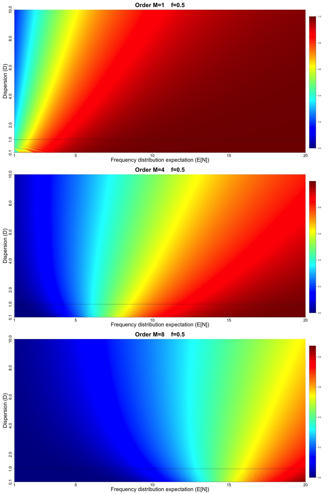
Figures 8, 9, and 10 display results analogous to Figure 7 but for higher loss threshold such that $f=0.8$, $f=0.9$, and $f=0.99$ respectively. Note that in all of Figures 7, 8, 9, and 10, we have intentionally not fixed the numerical scales associated with the different colors in the heat map to emphasize the shapes of the gradients in $D$ and $\mathbb{E}[N]$ space (which is the main focus of the discussion to follow).

Figure 8.Results in this figure are analogous to Figure 7, except that the chosen loss threshold corresponds to $f=0.8=\int_0^l f_X(x) d x$.

Figure 9.Results in this figure are analogous to Figure 7, except that the chosen loss threshold corresponds to $f=0.9=\int_0^l f_X(x) d x$.

Figure 10.Results in this figure are analogous to Figure 7, except that the chosen loss threshold corresponds to $f=0.99=\int_0^l f_X(x) d x$.

With Figures 7, 8, 9, and 10 in hand, we are able to make some interesting qualitative observations:

• For all values of $f$ and all orders $M$, higher rate implies increasing exceedance probability, and for high $f$ and high orders $M$, larger gains in exceedance probability are achieved for higher values of dispersion.

• For order $M=1$, we generally see that increasing dispersion leads to lower exceedance probability.

• As we progress to higher orders and more extreme values of loss thresholds (larger values of $f$) we see the rightward tilting exceedance probability surface changes to a leftward tilting surface. Therefore, for higher orders, we see that increasing dispersion increases exceedance probability (unlike the lowest order $M=1$). This has implications for pricing so-called catXL reinsurance contracts with multiple reinstatements, which attach at high loss thresholds.

• The more extreme the loss metric, the more pronounced the gain in exceedance probability is for increasing dispersion (seen for example by comparing Figures 8 and 9).

• Notice that in all panels of Figures 7, 8, 9, and 10, below the dispersion $D=1$ line, we see the effect of the numerical rounding inherent to the binomial model. This is particularly noticeable in Figure 7 where we see the appearance of “waves” in the exceedance probability surfaces below the $D=1$ line, attributable to the numerical rounding. This shows the consequences of the fact that we cannot smoothly cover the $D<1$ and $\mathbb{E}[N]$ space using the canonical frequency. Our results point to a potential advantage in using the Generalized Poisson and/or CMP to model the $D<1$ cases, as we presume that it is possible to smoothly cover the full $D$ and $\mathbb{E}[N]$ space. We imagine that if we were to plot the Sensitivity Spaces for the Generalized Poisson and CMP, they would look qualitatively similar, but without the appearance of numerical waves for $D<1$. This assertion is based on Figures 5 and 6, where our results hinted at the equivalence of the order statistic distributions derived from the Generalized Poisson and CMP in comparison with the canonical frequency.

Figures 7, 8, 9, and 10 collectively demonstrate how we can visualize sensitivity of important exceedance probability metrics to model assumptions. The mathematical result for the $F_{X_{M}}(l)$ in the case of the canonical frequency distribution (Proposition 3.4) is particularly useful in this context, as we can easily visualize many model configurations without the need for timeline simulations and other related approximations. We view Figures 7, 8, 9, and 10 as a demonstration of a top-down approach to understanding the implications of model changes to important loss metrics. In particular, such Sensitivity Spaces are conceptually useful in understanding the effects of changing model assumptions in the context of natural catastrophe reinsurance pricing. Similar types of analysis could be extended to address a broader set of questions; for example, what is the sensitivity to changes in the characteristics of the severity distribution itself? Our brief numerical treatment in this work motivates further exploration in this direction using societally relevant practical examples.

5. Practical application for quantifying the impacts of climate change on reinsurance pricing metrics

The Sensitivity Space plots in Figures 7, 8, 9, and 10 show the exceedance probabilities of various order statistics, for a variety of loss thresholds, and for a range of expected frequencies $\mathbb{E}\left[N\right]\in[1,20]$ and dispersion values $D\in[0.1,10]$. As discussed in Khare and Roy (2021), these exceedance probabilities are key to understanding which order statistics contribute to reinsurance pricing metrics. The higher the exceedance probability the higher the contribution of a given order statistic. Here we discuss how market practitioners can make use of our Sensitivity Space plots for given model output. We assume that one has access to catastrophe model output run against a particular portfolio prior to the application of a catXL reinsurance contract at a particular loss threshold $l$ of interest. We assume that this model output comes in the form of a timeline simulation or an event loss table (e.g., Homer and Li 2017).

One of the remarkable aspects of our results in Figures 7, 8, 9, and 10 is that the gradient of the order statistic exceedance probabilities (in the $\mathbb{E}\left[N\right]$ and $D$ direction) depends strongly on where in the $\mathbb{E}\left[N\right]$ and $D$ space our model sits for a given loss threshold and order $M$. For example, in Figure 7, for $D=1$, the change in the $M=1$ exceedance probability is small for $\mathbb{E}\left[N\right]\in[5,10]$ but much higher (in a relative sense) for the $M=2$ surface. Figure 8 reveals a different gradient for the same range of frequency $\mathbb{E}\left[N\right]\in[5,10]$ and $D=1$. In other words, the sensitivity of the exceedance probabilities of the order statistics depends on the model characteristics and the loss threshold of interest that corresponds to the attachment point of a given catXL contract. While our Figures 7, 8, 9, and 10 only cover four particular loss thresholds, similar Sensitivity Space plots can be made for any loss threshold of interest. The practical application of our Sensitivity Space plots boils down to computing the $\mathbb{E}\left[N\right]$ and $D$ for a given model output and determining the value of $f=\int_{0}^{l}f_{X}(x)dx$ for a given loss threshold $l$. We now provide a brief discussion of how to do so for two common forms of model output in the market.

5.1. Timeline simulation models

We assume that the timeline simulation model output is collected into a matrix $L_{N_{max},S}$ with $N_{max}$ rows and $S$ columns (number of simulation years as in Definition 2.8). $N_{max}$ is the maximum number of event occurrences across all simulation years $S$. The annual maximum losses are stored in the first row, and so on. The columns of $L_{N_{max},S}$ may contain $0$ values corresponding to years where the number of events is less than $N_{max}$. We assume all event occurrences have losses greater than $0$. Consistent with our assumption in Section 2, we assume frequency and severity are independent. Under this assumption, we can use the losses in $L_{N_{max,}S}$ to compute $\mathbb{E}\left[N\right]$, $D$, and $f$ (for a chosen loss threshold $l$). This requires the following steps:

• Compute a sample estimate of $\mathbb{E}\left[N\right]$ by counting the number of non-zero losses in $L_{N_{max},S}$ and dividing by $S$. Call this estimate $\hat{\mathbb{E}}\left[N\right]=\frac{N_{e}}{S}$, where $N_{e}$ is the number of non-zero loss events.

• For each year of simulation $i=1,...,S$, compute the number of events implied by $L_{N_{max},S}$ (by simply counting the number of non-zero losses per year). With these $S$ samples of $N$, compute the sample variance, and call it $\hat{\mathbb{V}}\left[N\right]$. The estimate of the dispersion is $\hat{D}=\frac{\hat{\mathbb{V}}\left[N\right]}{\hat{\mathbb{E}}\left[N\right]}$.

• To approximate the cumulative probability of the severity at loss threshold $l$, collect all the non-zero losses in $L_{N_{max},S}$ and place them in a vector $\overrightarrow{L}_{N_{e}}$ of dimension $N_{e}$. $\overrightarrow{L}_{N_{e}}$ is made up of random samples of the severity $f_{X}(x)$. For a given catXL contract with attachment point $l$, compute a sample estimate of $f=\int_{0}^{l}f_{X}(x)$ by determining the number of events in $\overrightarrow{L}_{N_{e}}$ that are less than $l$, and divide this by $N_{e}$. This is our sample estimate we call $\hat{f}$.

For the sake of this discussion, we assume that $\hat{f}$ is one of $0.5,0.8,0.9,0.99$ (to correspond to Figure 7, 8, 9, or 10). This need not be the case, as the Sensitivity Space plots can be recreated for any specific value of $f$ (or for that matter an expanded range of $\mathbb{E}\left[N\right],D$, and $M$). The next step is to look at the corresponding Figure 7, 8, 9, or 10 and determine which values of $\mathbb{E}\left[N\right]$, $D$ the model output from the timeline simulation corresponds to. The Sensitivity Space plots then enable us to determine the changes in the exceedance probabilities of the various order statistics in a region around the model for both changing expected frequency and dispersion. We note that the Sensitivity Space plots in Figures 7, 8, 9, and 10 correspond to the canonical frequency, but our contention is that qualitatively the results apply to generalized frequency distributions (given our results for the Generalized Poisson and CMP distributions). We leave aside the important question of the appropriate size of the region to look at in $\mathbb{E}\left[N\right]$, $D$ space to correspond to various climate change scenarios and time scales (we note that market practitioners can leverage commercial solutions for climate change models to help quantify this region). The above straightforward process makes use of sample statistics from the timeline simulation matrix $L_{N_{max},S}$. Next we discuss the use of event loss table model output.

5.2. Event loss table models

In this case, model output comes in the form of a matrix we call $E_{N_{e},3}$, which is an $N_{e}\times3$ matrix ($N_{e}$ here is distinct from the total number of events in the timeline simulation discussed above). The number of rows corresponds to the number of events $N_{e}$. The first row contains information about the first event. The first column (of the first row) corresponds to the average annual frequency of the first event, the second column is the mean loss given an occurrence of this event, and the third column is its standard deviation. Rows $2$ to $N_{e}$ in $L_{N_{e},3}$ have the same information for events $2$ to $N_{e}$. We assume the occurrences of the different events are independent. We also assume that, while the matrix $E_{N_{e},3}$ supplies the mean and standard deviation of the loss for each event, there is some parameterization, which gives an analytical probability density of loss for each event. Further, consistent with Section 2, we assume that for each individual event the frequency and severity are independent. Once again, to make use of the Sensitivity Space plots, we must compute estimates of $\mathbb{E}\left[N\right]$, $D$, and $f$ using the model output stored in $L_{N_{e},3}$:

• To obtain the estimate of $\mathbb{E}\left[N\right]$, simply sum the first column in the $E_{N_{e},3}$ matrix.

• The value of $D$ is dictated by the model formulation, and this information is not stored in the $E_{N_{e},3}$ matrix. For example, one could assume each individual event is Poisson (and therefore the overall frequency distribution is Poisson), which would imply that $D=1$.

• The average annual rates of the events are labelled as $\lambda_{i}$ where $i=1,...,N_{e}$. Given an event, assume the probability of getting a particular event $i$ is $p_{i}=\frac{\lambda_{i}}{\sum_{i=1}^{N_{e}}\lambda_{i}}$ (and $\sum_{i=1}^{N_{e}}p_{i}=1$). The severity is given by the probability weighted sum of the individual event severities which label as $f_{X_{i}}(x)$. The severity is a mixture model: $f_{X}(x)=\sum_{i=1}^{N_{e}}p_{i}f_{X_{i}}(x)$.

• Using the severity, numerical integration can be used to obtain an estimate of $f$ by numerically computing the integral $f=\int_{0}^{l}f_{X}(x)dx$.

With the above estimates of $\mathbb{E}\left[N\right]$, $D$, and $f$ in hand, one can follow a similar process to the one discussed above for timeline simulations to quantify model sensitivity to implied ranges from climate change (once again, sensible ranges to explore are available through commercial solutions).

6. Summary and Conclusions

This paper addresses the problem of quantifying changes to reinsurance pricing metrics arising from changes to frequency ($P_{N}(k)$) and severity ($f_{X}(x)$) assumptions. We are motivated by the notion that climate change implies changes to the underlying frequencies and severities (e.g., Knutson et al. 2020) that underpin technical reinsurance pricing. To do so we build on the results in Khare and Roy (2021), which demonstrate the importance of the order statistics in understanding the composition of catXL pricing metrics. In particular, Khare and Roy (2021) show that the exceedance probabilities (for a variety of loss thresholds) of the order statistics are one of the key drivers of technical pricing metrics. This paper augments Khare and Roy (2021) by demonstrating a framework to quantify changes to exceedance probabilities of the order statistics under changes to model assumptions. In particular we focus on changes arising from altered frequency ($P_{N}(k)$) distribution assumptions (although the same analysis can be extended to alterations in severity). Our framework enables one to explore the full range of dispersion values ($D\in(0,\infty)$) and average annual frequency ($\mathbb{E}\left[N\right]$).

This paper is focussed on the foundational and mathematical aspects of this problem, but we envision our study being useful as a basis for a variety of applied studies. As a first step we have provided a brief discussion on how to make use of results from model output commonly found in the market. The key contributions and conclusions from this paper are as follows:

• Section 3 provides a clear proof of the general formula of the cumulative probability of $X_{M}$ for a given frequency $P_{N}(k)$ and severity $f_{X}(x)$; the result is given in Theorem 3.2. We then reformulate the main result to write the cumulative probability as an explicit function of the cumulative probability of the annual maximum (one of the most commonly discussed distributions in practice). Our result is provided in Corollary 3.3}. We then apply the result from Corollary 3.3 to what we call the canonical frequency (negative binomial, Poisson, and binomial) which is able to “cover” the full range of dispersion values $D\in(0,\infty)$ (Definition 2.2). We achieve a closed form solution (Proposition 3.4) that can be used to rapidly explore the sensitivity of the $X_{M}$ exceedance probabilities to frequency model assumptions.

• Section 4 presents and discusses a novel set of numerical experiments. First, we compare and contrast the order statistics from the canonical frequency with those obtained using two particular generalized frequency distributions (Generalized Poisson and CMP). The generalized frequency distributions are able to cover the full dispersion range $D\in(0,\infty)$ without changes to the analytical form, which has advantages in various applications (Consul and Famoye 1990; Sellers and Shmueli 2010). Our results suggest that the generalized frequency distributions appear to generate nearly identical order statistics (which is useful background knowledge in applications of the generalized frequencies). In line with our stated goal of exploring sensitivity of exceedance probabilities of the order statistics to model assumptions, we also plot a series of Sensitivity Spaces (Figures 7, 8, 9, and 10) where we use the canonical frequency results from Proposition 3.4 to plot exceedance probabilities (for a variety of loss thresholds) as a function of the dispersion $D$, and the expectation of the frequency $P_{N}(k)$. From this we achieve a number of useful insights, discussed in the main text, that enable understanding of reinsurance pricing metrics under model changes. Our Sensitivity Space exercise also sheds further light on an issue with the canonical frequency that is likely to be overcome with one of the generalized frequency distributions studied here. In particular, for the case where $D<1$, the canonical exceedance probability surfaces suffer from the numerical approximation inherent to the use of the binomial distribution, which we contend can be alleviated by the use of the Generalized Poisson and/or CMP distributions.

• Section 5 discusses how practitioners can make use of model output commonly found in the market to address the impact of model changes on exceedance probabilities of the order statistics (motivated by our desire to quantify the impact of climate change on key reinsurance pricing metrics).

Our work can serve as a reference for practitioners interested in developing insights into reinsurance pricing under changing model assumptions. From the work in this paper, we envision a number of future studies of societal relevance. In particular, it would be interesting to use our methods for visualizing real-world examples from natural catastrophe risk models. For example, one could run a global suite of natural catastrophe models against the current-day economic exposure and establish a baseline portfolio-level frequency and severity. One could then perturb the model to capture changes to frequency, dispersion, and severity distribution characteristics under changing climates, and use our analytical results to understand changes to exceedance probabilities of $X_{M}$. One could do this exercise for a series of future economic scenarios, also capturing the uncertainty inherent to such projections. This type of work would serve to map out, at a high level, the implications of climate change on reinsurance pricing metrics.

Appendices

Appendix A: Proof of the general formula

By Definition 3.1,

$$F_{X_{M}}(l)=\sum_{k=0}^{\infty}P_{N}(k)F_{X_{M}}(l\mid N=k).$$

For $0\leq k\leq M-1$, we know that $F_{X_{M}}(l|N=k)=1$, since the random variable $X_{M}=0$ (the number of random events is always less than $M$). This yields

$$F_{X_{M}}(l)=\sum_{k=0}^{M-1}P_{N}(k)+\sum_{k=M}^{\infty}P_{N}(k)F_{X_{M}}(l\mid N=k).$$

We now focus on $k\geq M$ and compute $F_{X_{M}}(l|N=k)$ in the second sum immediately above. Using the binomial theorem we know that

$$(x+y)^{k}=\sum_{i=0}^{k}\left(\begin{array}{c} k\\ i \end{array}\right)x^{i}y^{k-i}$$

where $x,y$ are assumed to be real numbers and integer $k\geq1$. Let $x=1-f$ and $y=f$ (recall that $f\equiv\int_{0}^{l}f_{X}(x)dx$). In words, $y=f$ is the probability that an event has loss less than $l$, and $x=(1-f)$ is the probability that an event has loss greater than or equal to $l$. Plugging into the binomial theorem, we get

$$(f+1-f)^{k}=\sum_{i=0}^{k}\left(\begin{array}{c} k\\ i \end{array}\right)(1-f)^{i}f{}^{k-i}=1.$$

We can interpret the above equation in the context of timeline simulation. Suppose that, in a given year of timeline simulation, the realized number of events is $N=k\geq M$. Let the index $i$ represent the number of events greater than or equal to threshold $l$. The number of events greater than or equal to $l$ is at a minimum $0$ and at a maximum $k$ (there are exactly $k$ events). For any given $i$, $(1-f)^{i}$ is the probability associated with the configurations where $i$ of the total $k$ events is greater than or equal to $l$, and likewise $f^{k-i}$ is the probability associated with the configurations where $k-i$ events are less than $l$. Hence the expression

$$1=\sum_{i=0}^{k}\left(\begin{array}{c} k\\ i \end{array}\right)(1-f)^{i}f{}^{k-i}$$

accounts for all the configurations of $k$ events relative to the loss threshold $l$ and the probabilities associated with those configurations (adding up to $1$). We note that all possible configurations are accounted for given that $\left(\begin{array}{c} k\\ i \end{array}\right)$ quantifies the number of ways we can select $i$ events from the available $k$ events. Given that $k\geq M$, we can rewrite the above equation as

$$1=\sum_{i=0}^{M-1}\left(\begin{array}{c} k\\ i \end{array}\right)(1-f)^{i}f{}^{k-i}+\sum_{i=M}^{k}\left(\begin{array}{c} k\\ i \end{array}\right)(1-f)^{i}f{}^{k-i}.$$

We require cumulative probability of $X_{M}$ up to $l$, and we know that at most $M-1$ event losses can be greater than or equal to $l$. Therefore, the first sum on the right-hand side of the above equation is the probability we are seeking, so that

$$F_{X_{M}}(l|N=k)=\sum_{i=0}^{M-1}\left(\begin{array}{c} k\\ i \end{array}\right)(1-f)^{i}f{}^{k-i}.$$

Using the above results, we obtain the general formula

$$F_{X_{M}}(l)=\sum_{k=0}^{M-1}P_{N}(k)+\sum_{k=M}^{\infty}P_{N}(k)\sum_{i=0}^{M-1}\left(\begin{array}{c} k\\ i \end{array}\right)(1-f)^{i}f{}^{k-i}.$$

Appendix B: Proof of the alternative formulation

From Theorem 3.2, recall

$$F_{X_{M}}(l)=\sum_{k=0}^{M-1}P_{N}(k)+\sum_{k=M}^{\infty}P_{N}(k)\sum_{i=0}^{M-1}\left(\begin{array}{c} k\\ i \end{array}\right)(1-f)^{i}f{}^{k-i}.$$

We can write the second summation over index $k$ as starting from $0$, which requires that we subtract an additional term, to yield

$$\begin{aligned} F_{X_{M}}(l) & =\sum_{k=0}^{M-1}P_{N}(k)-\sum_{k=0}^{M-1}P_{N}(k)\sum_{i=0}^{M-1}\left(\begin{array}{c} k\\ i \end{array}\right)(1-f)^{i}f{}^{k-i}\\ & +\sum_{k=0}^{\infty}P_{N}(k)\sum_{i=0}^{M-1}\left(\begin{array}{c} k\\ i \end{array}\right)(1-f)^{i}f{}^{k-i}, \end{aligned}$$

noting that the factorial terms evaluate to $0$ when $i>k$. We now define the quantity $T$ given by the first two terms in the above equation:

$$T\equiv\sum_{k=0}^{M-1}P_{N}(k)-\sum_{k=0}^{M-1}P_{N}(k)\sum_{i=0}^{M-1}\left(\begin{array}{c} k\\ i \end{array}\right)(1-f)^{i}f{}^{k-i}.$$

Again note that $\left(\begin{array}{c} k\\ i \end{array}\right)$ evaluates to $0$ when $i>k$, hence $T$ can be written as

$$\begin{aligned} T & =\sum_{k=0}^{M-1}P_{N}(k)-\left[P_{N}(k=0)\sum_{i=0}^{0}\left(\begin{array}{c} 0\\ i \end{array}\right)(1-f)^{i}f{}^{-i}\right]\\ & -\left[P_{N}(k=1)\sum_{i=0}^{1}\left(\begin{array}{c} 1\\ i \end{array}\right)(1-f)^{i}f{}^{1-i}\right]\\ & -\left[P_{N}(k=2)\sum_{i=0}^{2}\left(\begin{array}{c} 2\\ i \end{array}\right)(1-f)^{i}f{}^{k-i}\right]\\ & +...\\ & -\left[P_{N}(k=M-1)\sum_{i=0}^{M-1}\left(\begin{array}{c} M-1\\ i \end{array}\right)(1-f)^{i}f{}^{M-1-i}\right], \end{aligned}$$

and notice that all the sums in the square brackets above evaluate to exactly 1 (binomial theorem), hence

$$\small{ \begin{align} T&=\sum_{k=0}^{M-1}P_{N}(k)\\ &\quad -\left[P_{N}(k=0)+P_{N}(k=1)+P_{N}(k=2)+...+P_{N}(k=M-1)\right]\\ &=0. \end{align} }$$

With $T=0$ we have

$$F_{X_{M}}(l)=\sum_{k=0}^{\infty}P_{N}(k)\sum_{i=0}^{M-1}\left(\begin{array}{c} k\\ i \end{array}\right)(1-f)^{i}f{}^{k-i},$$

and if we isolate the $i=0$ term, we obtain

$$F_{X_{M}}(l)=\sum_{k=0}^{\infty}P_{N}(k)f^{k}+\sum_{k=0}^{\infty}P_{N}(k)\sum_{i=1}^{M-1}\left(\begin{array}{c} k\\ i \end{array}\right)(1-f)^{i}f{}^{k-i},$$

which is

$$F_{X_{M}}(l)=F_{X_{1}}(l)+\sum_{k=0}^{\infty}P_{N}(k)\sum_{i=1}^{M-1}\left(\begin{array}{c} k\\ i \end{array}\right)(1-f)^{i}f{}^{k-i},$$

and, discarding the $i>k$ terms and rearranging the ordering of the sum (with impunity), we obtain the result

$$F_{X_{M}}(l)=F_{X_{1}}(l)+\sum_{i=1}^{M-1}\sum_{k=i}^{\infty}P_{N}(k)\left(\begin{array}{c} k\\ i \end{array}\right)(1-f)^{i}f{}^{k-i}.$$

Appendix C: Negative binomial

Here we prove Equation (3.4) for the negative binomial. Using the result from Proposition 3.3 and Equation (2.1) (with associated parameter definitions) we see that

$$\begin{aligned} F_{X_{M},nb}(l) & =\sum_{k=0}^{\infty}\frac{\Gamma(k+r)}{k!\Gamma(r)}p^{r}(1-p)^{k}f^{k}\\ & +\sum_{i=1}^{M-1}\sum_{k=i}^{\infty}\frac{\Gamma(k+r)}{k!\Gamma(r)}p^{r}(1-p)^{k}\left(\begin{array}{c} k\\ i \end{array}\right)(1-f)^{i}f{}^{k-i}. \end{aligned}$$

We now work out the first term on the right-hand side (the $F_{X_{1},nb}(l)$), which, after taking out the constant terms, becomes

$$F_{X_{1},nb}(l)=\frac{p^{r}}{\Gamma(r)}\sum_{k=0}^{\infty}\frac{\Gamma(k+r)(1-p)^{k}}{k!}f^{k},$$

and we find a closed form expression for the infinite sum using Mathematica programming language (“Wolfram Mathematica” 2023),

$$F_{X_{1},nb}(l)=\left(\frac{p}{1-f+fp}\right)^{r},$$

which, using $p=\frac{1}{D}$ and $r=\frac{\mu}{D-1}$, we see is

$$F_{X_{1},nb}(l)=\left(\frac{\frac{1}{OD}}{1-f+\frac{f}{OD}}\right)^{\frac{\mu}{D-1}},$$

which simplifies to

$$F_{X_{1},nb}(l)=\left(D(1-f)+f\right)^{\frac{\mu}{1-D}}.$$

Next we compute the second term on the right-hand side of the $F_{X_{M},nb}(l)$ expression above,

$$\scriptsize{ \begin{aligned} & \sum_{i=1}^{M-1}\sum_{k=i}^{\infty}\frac{\Gamma(k+r)}{k!\Gamma(r)}p^{r}(1-p)^{k}\frac{k!}{i!(k-i)!}(1-f)^{i}f{}^{k-i}\\ & =\sum_{i=1}^{M-1}\sum_{k=i}^{\infty}\frac{\Gamma(k+r)}{k!\Gamma(r)}p^{r}(1-p)^{k}\frac{k!}{i!(k-i)!}(1-f)^{i}f{}^{k-i}\\ & =\sum_{i=1}^{M-1}\frac{p^{r}(1-f)^{i}f^{-i}}{\Gamma(r)i!}\left[\frac{\Gamma(i+r)(1-p)^{i+0}f^{i+0}}{0!}+\frac{\Gamma(i+1+r)(1-p)^{i+1}f^{i+1}}{1!}+...\right]\\ & =\sum_{i=1}^{M-1}\frac{p^{r}(1-f)^{i}(1-p)^{i}}{\Gamma(r)i!}\left[\frac{\Gamma(i+r+0)(1-p)^{0}f^{i+0}}{0!}+\frac{\Gamma(i+r+1)(1-p)^{1}f^{1}}{1!}+...\right]\\ & =\sum_{i=1}^{M-1}\frac{p^{r}(1-f)^{i}(1-p)^{i}}{\Gamma(r)i!}\sum_{k=0}^{\infty}\frac{\Gamma(i+r+k)(1-p)^{k}f^{k}}{k!}. \end{aligned} }$$

We use Mathematica (“Wolfram Mathematica” 2023) to compute a closed form for the infinite sum,

$$\sum_{k=0}^{\infty}\frac{\Gamma(i+r+k)(1-p)^{k}f^{k}}{k!}=\frac{\Gamma(i+r)}{(1-f+fp)^{i+r}}.$$

So the general formula becomes

$$\begin{align} F_{X_{M},nb}(l)&=F_{X_{1},nb}(l)\\ &\quad+\sum_{i=1}^{M-1}\frac{p^{r}(1-f)^{i}(1-p)^{i}}{\Gamma(r)i!}\frac{\Gamma(i+r)}{(1-f+fp)^{i+r}}. \end{align}$$

But we can factor out $\frac{p^{r}}{(1-f+fp)^{r}}$ from the second term on the right-hand side to obtain (and recognizing this as the $F_{X_{1},nb}(l)$)

$$\begin{align} F_{X_{M},nb}(l)&=F_{X_{1},nb}(l)\\ &\quad +F_{X_{1},nb}(l)\sum_{i=1}^{M-1}\frac{(1-f)^{i}(1-p)^{i}}{\Gamma(r)i!}\frac{\Gamma(i+r)}{(1-f+fp)^{i}}, \end{align}$$

and again using the fact that $p=\frac{1}{D}$, $r=\frac{\mu}{D-1}$, and $\mathbb{E}\left[N\right]=\mu$, we see after some straightforward work that the final form completing the proof is

$$\small{ \begin{align} &F_{X_{M},nb}(l)\\ &\quad=F_{X_{1},nb}(l)\left(1+\sum_{i=1}^{M-1}\frac{\Gamma(i+\frac{\mathbb{E}\left[N\right]}{D-1})}{\Gamma(\frac{\mathbb{E}\left[N\right]}{D-1})i!}\left(\frac{D(1-f)+f-1}{D(1-f)+f}\right)^{i}\right). \end{align} }$$

Note that $F_{X_{1},nb}(l)=\left(D(1-f)+f\right)^{\frac{\mu}{1-D}}=\left(D(1-f)+f\right)^{\frac{\mathbb{E}\left[N\right]}{1-D}}.$

Appendix D: Poisson

Here we prove Equation (3.5) for the Poisson case. Starting with the general formula in Corollary 3.3 (for $M\geq2$) and Equation (2.2) (with associated parameter definition),

$$\begin{align} F_{X_{M},pois}(l)&=\sum_{k=0}^{\infty}\frac{e^{-\lambda}\lambda^{k}}{k!}f^{k}\\ &\quad +\sum_{i=1}^{M-1}\sum_{k=i}^{\infty}\frac{e^{-\lambda}\lambda^{k}}{k!}\left(\begin{array}{c} k\\ i \end{array}\right)(1-f)^{i}f^{k-i}, \end{align}$$

we use Mathematica (“Wolfram Mathematica” 2023) to compute the first term on the right-hand side, which is the $F_{X_{1},pois}(l)$ given by

$$F_{X_{1},pois}(l)=e^{-\lambda(1-f)}.$$

We now compute the second term on the right-hand side of the $F_{X_{M},pois}(l)$ equation above in a series of steps:

$$\small{ \begin{aligned} & \sum_{i=1}^{M-1}\sum_{k=i}^{\infty}\frac{e^{-\lambda}\lambda^{k}}{k!}\left(\begin{array}{c} k\\ i \end{array}\right)(1-f)^{i}f^{k-i}\\ & =\sum_{i=1}^{M-1}\sum_{k=i}^{\infty}\frac{e^{-\lambda}\lambda^{k}}{k!}\frac{k!}{(k-i)!i!}(1-f)^{i}f^{k-i}\\ & =\sum_{i=1}^{M-1}\frac{e^{-\lambda}(1-f)^{i}f^{-i}}{i!}\sum_{k=i}^{\infty}\frac{\lambda^{k}}{(k-i)!}f^{k}\\ & =\sum_{i=1}^{M-1}\frac{e^{-\lambda}(1-f)^{i}f^{-i}}{i!}\left[\frac{\lambda^{i}f^{i}}{0!}+\frac{\lambda^{i+1}f^{i+1}}{1!}+\frac{\lambda^{i+2}f^{i+2}}{2!}+...\right]\\ & =\sum_{i=1}^{M-1}\frac{e^{-\lambda}(1-f)^{i}}{i!}\left[\frac{\lambda^{i}}{0!}+\frac{\lambda^{i+1}f^{1}}{1!}+\frac{\lambda^{i+2}f^{2}}{2!}+...\right]\\ & =\sum_{i=1}^{M-1}\frac{(1-f)^{i}\lambda^{i}}{i!}\left[\frac{e^{-\lambda}(\lambda f)^{0}}{0!}+\frac{e^{-\lambda}(\lambda f)^{1}}{1!}+\frac{e^{-\lambda}(\lambda f)^{2}}{2!}+...\right]\\ & =\sum_{i=1}^{M-1}\frac{(1-f)^{i}\lambda^{i}}{i!}\left(\sum_{k=0}^{\infty}\frac{e^{-\lambda}\lambda^{k}}{k!}f^{k}\right). \end{aligned} }$$

We recognize the infinite sum above as the $F_{X_{1},pois}(l)$, hence

$$F_{X_{M},pois}(l)=F_{X_{1},pois}(l)+F_{X_{1},pois}(l)\sum_{i=1}^{M-1}\frac{(\lambda(1-f))^{i}}{i!},$$

and noting that $\mathbb{E}\left[N\right]=\lambda$ we see the final form that completes the proof is

$$F_{X_{M},pois}(l)=F_{X_{1},pois}(l)\left(1+\sum_{i=1}^{M-1}\frac{(\mathbb{E}\left[N\right](1-f))^{i}}{i!}\right).$$

Note that $F_{X_{1},pois}(l)=e^{-\lambda(1-f)}=e^{-\mathbb{E}\left[N\right](1-f)}$.

Appendix E: Binomial

Here we prove Equation (3.6) for the binomial distribution. Using the general formula from Corollary 3.3 and Equation (2.1) (with associated parameter definitions),

$$\small{ \begin{align} F_{X_{M},bn}(l)&=\sum_{k=0}^{\infty}\left(\begin{array}{c} n\\ k \end{array}\right)q^{k}(1-q)^{n-k}f^{k}\\ &\quad +\sum_{i=1}^{M-1}\sum_{k=i}^{\infty}\left(\begin{array}{c} n\\ k \end{array}\right)q^{k}(1-q)^{n-k}\left(\begin{array}{c} k\\ i \end{array}\right)(1-f)^{i}f^{k-i}. \end{align} }$$

We now compute the first term on the right-hand side (the $F_{X_{1},bn}(l)$), noting that we must have $k\leq n$ so the infinite sum becomes

$$F_{X_{1},bn}(l)=\sum_{k=0}^{n}\left(\begin{array}{c} n\\ k \end{array}\right)q^{k}(1-q)^{n-k}f^{k},$$

which can be rewritten in a suggestive form,

$$F_{X_{1},bn}(l)=\sum_{k=0}^{n}\left(\begin{array}{c} n\\ k \end{array}\right)(1-q)^{n-k}\left(qf\right)^{k},$$

where by the binomial theorem we see that

$$F_{X_{1},bn}(l)=(1-q+qf)^{n}.$$

We now compute the second term on the right-hand side of $F_{X_{M},bn}(l)$ in a series of steps (we call this term $A$). Once again, we must have $k\leq n$ so we can truncate the infinite sum to obtain

$$A=\sum_{i=1}^{M-1}\sum_{k=i}^{n}\left(\begin{array}{c} n\\ k \end{array}\right)q^{k}(1-q)^{n-k}\left(\begin{array}{c} k\\ i \end{array}\right)(1-f)^{i}f^{k-i}.$$

We factor out the $(1-q)^{n}$ to obtain

$$A=(1-q)^{n}\sum_{i=1}^{M-1}\sum_{k=i}^{n}\left(\begin{array}{c} n\\ k \end{array}\right)q^{k}(1-q)^{-k}\left(\begin{array}{c} k\\ i \end{array}\right)(1-f)^{i}f^{k-i},$$

and we can use Mathematica (“Wolfram Mathematica” 2023) to compute the sum over $k$ to obtain

$$\small{ A=(1-q)^{n}\sum_{i=1}^{M-1}\left(\begin{array}{c} n\\ i \end{array}\right)\left(-1+\frac{1}{f}\right)^{i}\left(\frac{fq}{1-q}\right)^{i}\left(\frac{-1+q-fq}{-1+q}\right)^{-i+n}, }$$

after which we can take out the term raised to the power of $n$ within the sum to get

$$\small{ A=(1-q+qf)^{n}\sum_{i=1}^{M-1}\left(\begin{array}{c} n\\ i \end{array}\right)\left(-1+\frac{1}{f}\right)^{i}\left(\frac{fq}{1-q}\right)^{i}\left(\frac{1-q+qf}{1-q}\right)^{-i}, }$$

and, returning to the general formula and with some straightforward simplifications of the above term, we see that

$$F_{X_{M},bn}(l)=F_{X_{1},bn}(l)\left(1+\sum_{i=1}^{M-1}\left(\begin{array}{c} n\\ i \end{array}\right)\left(\frac{(1-f)q}{1-q+qf}\right)^{i}\right).$$

Using the fact that $D=1-q$ and $n=\frac{\mathbb{E}\left[N\right]}{1-D}$, we obtain the final form that completes the proof,

$$\small{ F_{X_{1},bn}(l)=F_{X_{1},bn}(l)\left(1+\sum_{i=1}^{M-1}\left(\begin{array}{c} \frac{\mathbb{E}\left[N\right]}{1-D}\\ i \end{array}\right)\left(\frac{(1-f)(1-OD)}{OD+(1-OD)f}\right)^{i}\right). }$$

Note that $F_{X_{1},bn}(l)=(1-q+qf)^{n}=(D+(1-D)f)^{\frac{\mathbb{E}\left[N\right]}{1-D}}$.