Matrix Variate Regression as a Tool for Insurers

1. Introduction

1.1. Three-way data

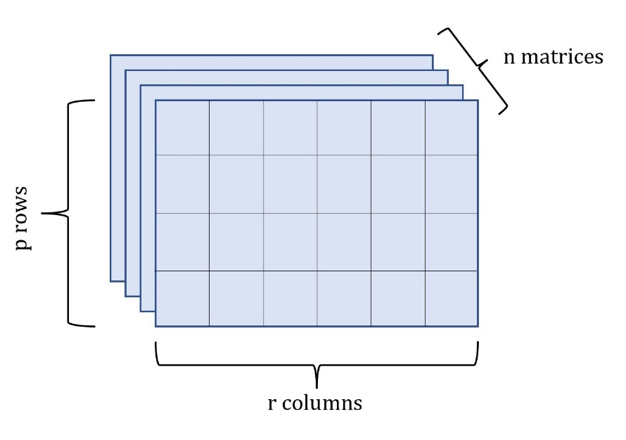
Regressions with univariate and multivariate responses are among the most straightforward and intuitive modeling tools available to insurers. Univariate regression analysis is frequently used in loss reserving, ratemaking, and financial modeling (Cerchiara 2021; Taylor and McGuire 2016; Frees 2009). Regression with multivariate response is more general in that it allows the modeler to account for multiple response variables at once, and estimate the covariance between each type of response (Johnson and Wichern 2007). In practice, however, there are situations in which each single observation of the response in a dataset constitutes a realization of a random matrix. This situation arises in time series or spatial datasets where each response consists of multiple metrics measured across time or space, or when variables can be stratified across three different dimensions. We call this type of data three-way data (Coppi et al. 1989).

Figure 1.Example of a Three-Way (Matrix Variate) Dataset

Each observation of a response variable in a three-way data set is a matrix. For example, each of the n responses (matrices) in the dataset could hold dollar losses from p different lines of business in r different locations in a particular year.

In these instances, there may be dependency in the response variable across the stratified dimensions of the matrix, such as time or space. When this type of data is treated as a univariate or multivariate response, the dependency among the dependent variable violates one of the basic assumptions in regression contexts: independent observations. Thus, univariate and multivariate regression are not able to capture the rich dependence structure that arises in three-way datasets. While univariate distributions can be used to build models for univariate response data (one-way data), and multivariate distributions apply in the case of multivariate response (two-way) data, a great deal of study has focused on matrix variate distributions, which apply to matrix variate response data (three-way) data (Gupta and Nagar 1999).

To better explain three-way data, consider a dataset consisting of losses from $p$ different lines of insurance, stratified across $r$ geographical areas. This data can naturally be arranged in a single $p \times r$ matrix. Now, if we observe losses stratified in this manner for $n$ consecutive years, the result is a length $n$ time series of $p \times r$ matrices. In fact, in this article, we will explore a particular example and analyze a time series of property losses from $p = 4$ different natural hazards across $r = 4$ regions of the U.S for $n = 60$ years. In this example, there is dependency in the response variable along the $p$ different lines of insurance, and across $r$ geographical areas. Matrix variate regression is well suited to this type of problem because it is able to account for these correlated responses.

A growing number of insurance problems require modeling the distributions of random matrices. The most commonly used distribution within the finance and actuarial literature is the Wishart distribution (Wishart 1928), which arises as the distribution of the sample covariance matrix of a multivariate normal dataset. The Wishart distribution has widely been applied in insurance and finance problems such as portfolio analysis (Bodnar, Mazur, and Podgorski 2016), time series analysis (Gourieroux, Jasiak, and Sufan 2009), and ratemaking (Chiarella, Da Fonseca, and Grasse 2014). For example, Denuit and Lu (2021) considered Wishart-gamma random effects to model serially correlated insurance claim data. Other approaches in the actuarial literature to capture complex dependency structures include a copula method developed by Shi, Lee, and Maydeu-Olivares (2019), and a credibility premium formula proposed by Jeong and Dey (2021) for claims from multiple lines of business. However, many matrix variate distributions exist, such as the matrix variate normal and matrix variate t distributions, and their use to capture dependency structures has not been explored yet within the actuarial domain.

In this paper, we describe the matrix variate regression model, revealing its suitability to a wide variety of insurance applications. Also, we provide an instructive example by giving a particular use case of the methodology, allowing for the simultaneous modeling of the temporal and spatial dimension of losses from a variety of natural disasters given a matrix of covariates. In this introductory work, we focus on modeling using the matrix variate normal distribution, although extensions can be made to other matrix variate distributions in order to allow for non-symmetric or heavy tailed data.

1.2. The matrix variate normal distribution

In the linear regression context, the errors are typically assumed to be distributed according to a univariate or multivariate normal distribution. Thus, the matrix variate normal distribution (Gupta and Nagar 1999) provides a natural first choice for the matrix variate regression. A $p \times r$ matrix $Y$ is matrix variate normally distributed when its probability density function is specified by:

$$\scriptsize{ \begin{align} &f_{p,r}\left( Y|M,\Sigma,\ \Psi \right) \\ &\quad = (2\pi)^{- \frac{pr}{2}}|\Sigma|^{- \frac{r}{2}}|\Psi|^{- \frac{p}{2}}etr( - \frac{1}{2}\Sigma^{- 1}(Y - M)\Psi^{- 1}(Y - M)^{'}) \end{align} \tag{1.1} }$$

where $M$ is the mean matrix, and the two matrices $\Sigma$ and $\Psi$ represent the within-row covariance and within-column covariances, respectively^[1]. If the matrix $Y$ is matrix variate normally distributed, we write $Y\sim N_{p,r}(M,\Sigma,\Psi)$. This matrix normal distribution can be seen as a natural extension of the multivariate normal distribution. The relationship between the two can be seen further through the so-called vectorization function, which structures the matrix into a single vector by stacking columns on top of one another. In fact, if $Y$ is matrix variate normally distributed, its vectorized form has the multivariate normal distribution: $vec(Y)\sim N_{pr}\left( vec(M),\Psi \otimes \Sigma \right)$. Here, $\otimes$ represents the Kronecker product, which multiplies each entry of $\Psi$ by the matrix $\Sigma$. The result is a $pr \times pr$ matrix:

$$\Psi \otimes \Sigma = \ \begin{bmatrix} \Psi_{11}\Sigma & \cdots & \Psi_{1r}\Sigma \\ \vdots & \ddots & \vdots \\ \Psi_{r1}\Sigma & \cdots & \Psi_{rr}\Sigma \end{bmatrix}.$$

While the matrix variate regression model and its vectorized form are related, the benefit of the matrix variate approach over the multivariate vectorized form is that separate estimates are obtained for $\Sigma$ and $\Psi$ rather than solely an estimate of the Kronecker product $\Psi \otimes \Sigma$. For this reason, we say that the matrix variate dataset has a separable covariance structure. This kind of modeling allows one to make inferences separately, but simultaneously, for the covariances between the two dependent dimensions.

As an example, consider a data set comprised of $p \times r$ matrices, containing $r$ repeated measures of $p$-variate observations. In this case, $\Sigma$ would contain the covariances between the $p$ dependent variables (the rows of the matrices), while $\Psi$ would contain the covariances between the $r$ repeated measures (the columns of the matrices).

Alternatively, consider again the matrix variate time series consisting of losses from $p$ lines of business stratified across $r$ locations, as depicted in Figure 1. In this case, $\Sigma$ would contain the covariances of losses between the $p$ lines of business, while $\Psi$ would contain the covariances between the $r$ locations.

A number of recent works have illustrated how this variance structure can be exploited within a typical regression context (Viroli 2012; Anderlucci, Montanari, and Viroli 2014; Ding and Cook 2018; Melnykov and Zhu 2019). In this instance, a matrix of covariates, $X_{i}$ are used to model an output matrix, ${\widehat{Y}}_{i}$. Here, the primary assumption is the separable covariance structure for the errors of the model.

One primary benefit of employing the matrix variate distribution within a modeling context is this covariance structure for the model errors. In classical regression contexts, independence of errors is a necessary modeling assumption. However, in many scenarios this is not the case. Consider again the example of losses from different lines of insurance stratified across locations. Here, we may have dependency in losses between the different lines of business and between locations. In a univariate or multivariate response approach, a dependency structure would need to be chosen and incorporated into the model to account for non-independent errors. The matrix variate approach naturally allows for dependency between rows and columns, without needing to choose any particular dependency structure in the errors for each.

When presented with a matrix variate dataset, a modeler may choose simply to work with the vectorized form, applying typical multivariate response modeling techniques. However, the matrix variate distribution provides not only an intuitive structure, but also a more parsimonious model than this multivariate response counterpart. This is because the covariance matrix in the multivariate response approach is completely unrestricted, with a number of entries, and thus parameters to be fit, equal to $\frac{pr(pr + 1)}{2}$. Meanwhile, the matrix variate covariance structure assumes separability of the covariance into the two matrices $\Sigma$ and $\Psi$, whose Kronecker product gives the corresponding multivariate covariance matrix. Thus, the number of total entries in these two matrices is given by $\frac{p(p + 1)}{2} + \frac{r(r + 1)}{2}$ , which is a marked reduction in the number of parameters to be fit from the unrestricted multivariate model (Viroli 2012).

2. Matrix variate regression

2.1. The model

The model presented here was developed in (Viroli 2012) and (Ding and Cook 2018). Assume we have a dataset of $n$ response observations of $p \times r$ matrices. We introduce the matrix variate regression model as follows:

$$Y_{i} = \mu + \beta_{1}X_{i}\beta_{2}^{'} + \epsilon_{i} \tag{2.1}$$

Here, $Y_{i}$ is a $p \times r$ matrix of responses, and $X_{i}$ is a standardized $q_{1} \times q_{2}$ matrix associated with response $i$ containing $q_{1}$ independent variables stratified in $q_{2}$ ways. For example, the $X_{i}$ matrix could hold $q_{1}$ predictors measured at $q_{2}$ locations, or for $q_{2}$ time periods. The model parameters are contained in the matrices $\mu$, $\beta_{1}$, and $\beta_{2}$, where $\mu$ is the $p \times r$ mean response, and $\beta_{1}$ (dimension $p \times q_{1}$) and $\beta_{2}$ (dimension $r \times q_{2}$) are matrices of coefficients. We also have that $\epsilon_{i}$ is an error matrix for observation $i$, which is assumed to be matrix variate normally distributed with mean matrix $0$ and covariance matrices $\Sigma$ and $\Psi$, having $\epsilon_{i}\sim N_{p,r}(0,\Sigma,\ \Psi)$.

Just as the covariance matrix can be separated to estimate the covariance between the rows and columns separately, so also in this model the coefficients are separated into matrices $\beta_{1}$ and $\beta_{2}$. The matrix $\beta_{1}$ contains the coefficients relating the predictors to the rows of the response matrix, while $\beta_{2}$ provides information about how the predictors affect the columns of the response matrix. To illustrate why this is the case, consider altering the $ij^{th}$ entry of $\beta_{1}$, denoted $\beta_{1}^{ij}$. Then all entries of row $i$ in the resulting matrix $\beta_{1}X_{i}\beta_{2}^{'}$ will be affected, while the other rows remain unchanged. Similarly, if we alter the $ij^{th}$ entry of $\beta_{2}^{'}$, then all entries of column $j$ in the resulting matrix $\beta_{1}X_{i}\beta_{2}^{'}$ will be affected, while the other columns remain the same. Further, as seen in (Gupta and Nagar 1999), applying the properties $vec(A + B) = vec(A) + vec(B)$ and $vec(ABC) = \ C^{'} \otimes B\ vec(A)$ , we have:

$$\begin{align} vec\left( Y_{i} \right) &= vec(\mu) + \beta_{2} \otimes \beta_{1}vec\left( X_{i} \right) \\ &\quad + vec(\epsilon_{i}) \end{align} \tag{2.2}$$

Thus, the matrix $\beta_{2} \otimes \beta_{1}$ gives the coefficients that relate the entries of $X_{i}$ to the response matrix. Thus, the approach harnesses the structural information of both the response matrix and the predictors, allowing for data sharing among the same row/column in modeling each element of the response.

The matrix variate model proposed in (2.1) covers a wide variety of different models, with both univariate and multivariate response regression models as special cases. For example, if the response matrix has dimensions $1 \times 1$, then the model reduces to the univariate case, while if the response matrix is of dimension $p \times 1$ or $1 \times r$, the model reduces to the multivariate response case. In any of these cases, the independent variables (i.e. covariates or predictors) contained in $X_{i}$ can constitute a matrix, a vector, or a univariate independent variable, depending on the dimensions of $X_{i}$. Thus, one could devise for example, a univariate model with matrix variate inputs, or a matrix variate model with multivariate predictors, or any other such combination. A selection of special cases will be further explored in Section 3.3.

2.2. Parameter estimation

Parameter estimation follows from maximum likelihood approach. An alternative to least squares estimation, the maximum likelihood method estimates the parameters by finding the values that maximize the likelihood of observing the given dataset. This is accomplished by maximizing the log-likelihood function, which is for this model is specified as:

$$\scriptsize{ \begin{aligned} &l\left(M, \Sigma, \Psi \mid Y_i, X_i\right)\\ &\quad= c-\frac{n p}{2} \log |\Psi|-\frac{n r}{2} \log |\Sigma|\\ &\qquad -\frac{1}{2} \sum_{i=1}^n \operatorname{tr}\left\{\Sigma^{-1}\left(Y_i-\mu-\beta_1 X_i \beta_2^{\prime}\right) \Psi^{-1}\left(Y_i-\mu-\beta_1 X_i \beta_2^{\prime}\right)^{\prime}\right\} \end{aligned} \tag{2.3} }$$

Here, c is a constant, which will not impact parameter fitting. Maximization of this function leads to the estimates in (2.4-2.8).

$$\widehat{\mu} = \overline{Y}\tag{2.4}$$

$$\small{ \widehat{\beta_{1}} = \left\lbrack \sum_{i = 1}^{n}{\left( Y_{i} - \overline{Y} \right){\widehat{\Psi}}^{- 1}{\widehat{\beta}}_{2}X_{i}^{'}} \right\rbrack\left\lbrack \sum_{i = 1}^{n}{X_{i}{\widehat{\beta}}_{2}^{'}{\widehat{\Psi}}^{- 1}{\widehat{\beta}}_{2}X_{i}^{'}} \right\rbrack^{- 1}\tag{2.5} }$$

$$\small{ \widehat{\Sigma} = \frac{1}{nr}\sum_{i = 1}^{n}{(Y_{i} - \overline{Y}} - {\widehat{\beta}}_{1}X_{i}{\widehat{\beta}}_{2}^{'}){\widehat{\Psi}}^{- 1}(Y_{i} - \overline{Y} - {\widehat{\beta}}_{1}X_{i}{\widehat{\beta}}_{2}^{'})'\tag{2.6} }$$

$$\small{ \widehat{\beta_{2}} = \left\lbrack \sum_{i = 1}^{n}{\left( Y_{i} - \overline{Y} \right)^{'}{\widehat{\Sigma}}^{- 1}\ {\widehat{\beta}}_{1}X_{i}} \right\rbrack\left\lbrack \sum_{i = 1}^{n}{X_{i}^{'}{\widehat{\beta}}_{1}^{'}{\widehat{\Sigma}}^{- 1}{\widehat{\beta}}_{1}^{'}X_{i}} \right\rbrack^{- 1}\tag{2.7} }$$

$$\scriptsize{ \widehat{\Psi} = \frac{1}{np}\sum_{i = 1}^{n}{(Y_{i}^{'} - {\overline{Y}}^{'}} - {\widehat{\beta}}_{2}X_{i}^{'}{\widehat{\beta}}_{1}^{'}){\widehat{\Sigma}}^{- 1}(Y_{i} - \overline{Y} - {\widehat{\beta}}_{1}X_{i}{\widehat{\beta}}_{2}^{'})\ \tag{2.8} }$$

Here, $\overline{Y}$ represents the mean matrix of all $Y_{i}$ matrices. In addition, the hat notation represents an estimated fit parameter; for example, ${\widehat{\beta}}_{1}$ represents the fit parameter for $\beta_{1}$. Details of this derivation are available from supplemental materials to (Ding and Cook 2018). Fully analytical solutions are not available for all parameters. Instead, estimation is done iteratively. First, $\mu$ is estimated as in (2.4). Next, an initial random estimate is assigned to ${\widehat{\beta}}_{2}$ and $\widehat{\Psi}$. Then using the equations in (2.5) and (2.6) estimates are obtained for ${\widehat{\beta}}_{1}$ and $\widehat{\Sigma}$. Having obtained these, ${\widehat{\beta}}_{2}$ and $\widehat{\Psi}$ are refit according to (2.7) and (2.8). The algorithm continues to update the estimates iteratively using (2.5-2.8) until the parameters converge.

It is important to note that $\Sigma$ and $\Psi$ are only defined up to a multiplicative constant. This is because if $\frac{1}{a}\widehat{\Sigma}$ and $\widehat{\Psi}$ are estimates of $\Sigma$ and $\Psi$, then we have $\widehat{\Psi} \otimes \frac{1}{a}\widehat{\Sigma} = \frac{1}{a}\widehat{\Psi} \otimes \widehat{\Sigma}$. Thus, $\widehat{\Sigma}$ and $\frac{1}{a}\widehat{\Psi}$ are also estimates of $\Sigma$ and $\Psi$. For this reason, we should impose an identifiability condition to ensure the estimates are unique. For example, we could scale the estimates so that the first element of $\Sigma$ is 1. Another option is to set the Frobenius^[2] norm of the matrix to 1, which is adopted in this paper. This identifiability condition will also need to be imposed on $\beta_{1}$ and $\beta_{2}$, which are also only unique up to a multiplicative constant. These imposed conditions do not affect the predictions ${\widehat{Y}}_{i}$. However, interpretations of $\beta_{1}$ and $\beta_{2}$ must be made with particular caution.

3. Application to natural hazard losses

Matrix variate regression can be applied to many insurance problems in P&C. When it comes to loss modeling, it allows one to analyze how losses from different risks interact, stratified in up to three dimensions. Here we consider dollar losses from natural hazards in different geographical locations. In the context of climate change and its effects on the distribution of losses from natural catastrophes, this modeling approach grants unique exploration of the evolving landscape of these risks while accounting for multiple sources of correlation within the data.

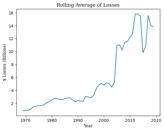
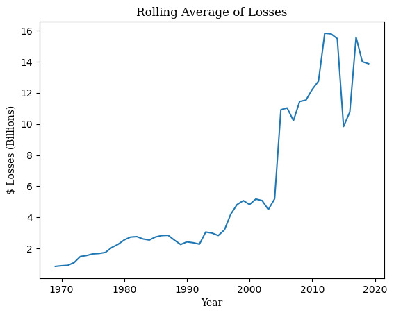
Between 1960 and 2019, natural hazards accounted for an annual average of $15.8 billion (2019 adjusted) in direct property losses and $3.3 billion (2019 adjusted) in crop losses, as well as determining approximately 583 deaths and 4,206 injury cases per year (CEMHS 2020). These impacts have been steadily increasing, with an average yearly increase of over $83 million (2019 adjusted) in property losses from 1960 to 2019 (calculated from SHELDUS dataset, CEMHS 2020). This increase may be impacted by a variety of economic factors, such as population growth and increased wealth. However, many scientists and reinsurers suspect that the main determinant is the increasing frequency and severity of catastrophic events due to climate change (IPCC 2001; Miller, Muir-Wood, and Boissonnade 2008).

Our analysis considers the annual direct property losses from four different hazards: flooding, hail, lightning, and wind. These losses are stratified across four regions of the United States as defined by the U.S. Census Bureau: the Midwest, the Northeast, the South, and the West (U.S. Census Bureau 2021). These two dimensions, hazard types and regions, form our rows and columns of the matrix response, respectively. Our dataset, then, consists of a time series of $n = 60$ matrix variate responses of dimension $4 \times 4$, each containing aggregate losses from four different hazard types in four regions of the U.S.

Figure 2.Rolling Average of Losses

Dollar losses in billions from flood, hail, lightning, and wind events from 1960-2019, averaged over 10-year intervals.

3.1. Data

Loss data for this analysis comes from the SHELDUS database (CEMHS 2020) which contains estimated direct losses from a variety of natural hazards and perils for the period from 1960 through 2019. Originally developed by the Hazards and Vulnerability Research Institute at the University of South Carolina, SHELDUS is currently funded and maintained by the ASU Center for Emergency Management and Homeland Security (ASU 2021) and is updated annually. Much of the data is sourced from the National Centers for Environmental Information Storm Data, having undergone necessary cleaning and disaggregation (National Climatic Data Center et al. 2021).

The underlying loss data retrieved from SHELDUS is converted into U.S. 2019 dollars and scaled to be per capita in order to neutralize the effects of inflation and population growth. This data is structured into the response matrices $Y_{i}$, as exemplified in Tables 1 and 2.

To account for climatic variables, we collected the minimum, maximum, and average temperature, as well as the precipitation levels for each region yearly from The Global Historical Climatology Network daily database (NOAA National Centers for Environmental Information). In addition, number of wind events with windspeed above 40 knots was gathered from National Centers for Environmental Information Storm Data (National Climatic Data Center et al. 2021).

3.2. Model and results

Our response matrices consist of the log-losses per capita in 2019 adjusted dollars observed from flooding, hail, lightning, and wind, in the US Northeast, South, Midwest, and West. Details of the 8 included predictors are outlined in Table 3. We consider each of the 8 predictors measured for each of the 4 regions, resulting in $X_{i}$ of dimension $8 \times 4$ for each time period $i.$ Note that this predictor matrix could be constructed differently based on the use case, as described in Section 2.1. For example, if stratified predictor values were not available, $X_{i}$ could instead take dimension $8 \times 1$. An example $X_{i}$ matrix used in our analysis is given in Table 4. Prior to model fit, the covariate matrix was standardized entry-by-entry across observations.

Note that unlike in the case of univariate and multivariate models, the parameter fitting for the matrix variate model follows an iterative convergence algorithm. Iterative likelihood algorithms such are prone to converging at a local, rather than global, maximum. When the likelihood surface is complex, the fit parameters can be strongly influenced by their initial values, making it necessary to explore a larger number of random initializations for a comprehensive analysis. For this reason, for we randomly re-initialized the parameters 500 times, and the model was selected that resulted in the highest likelihood. Convergence was determined when the norm of the change of the matrix was below the threshold $10^{- 5}$ for all 4 fit matrices.

The two parameter matrices $\beta_{1}$ and $\beta_{2}$ allow for rich understanding of the underlying data relationships. However, special care must be taken when interpreting the estimated coefficients in $\beta_{1}$ and $\beta_{2}$ because these two matrices are only defined up to a multiplicative constant. Because the predictor matrix is standardized prior to model fitting, the structure of the individual matrices $\beta_{1}$ and $\beta_{2}$ can be used to understand the relative impact of the predictors on the row and column dimensions. Since these entries can be arbitrarily rescaled, they cannot on their own be used to quantify the impact on dollar loss. Instead, to quantify the impact of a particular predictor on a particular entry in the response matrix, $Β = \beta_{2} \otimes \beta_{1}$ is used, since this Kronecker product is uniquely defined. Notice that due to the structure of $Β,$ the effect of variable $X_{i}(j,k)$ on entry $l,m$ of matrix $\widehat{Y_{i}}$ is given by ${\widehat{\beta}}_{1}(l,j) \times {\widehat{\beta}}_{2}(k,m)$.

Thus, analysis of the impact of a particular predictor $X_{i}(j,k)$ on a particular entry $l,m$ in the response matrix can be aided by 3 steps: inspection of ${\widehat{\beta}}_{1}$, inspection of ${\widehat{\beta}}_{2},$ and estimation of impact on dollar losses. Here we illustrate with a concrete example: analyzing the impact of income in the Midwest on log-losses from flood events in the Midwest.

Thus, analysis of the impact of a particular predictor $X_{i}(j,k)$ on a particular entry $l,m$ in the response matrix can be aided by 3 steps: inspection of ${\widehat{\beta}}_{1}$, inspection of ${\widehat{\beta}}_{2},$ and estimation of impact on dollar losses. Here we illustrate with a concrete example: analyzing the impact of income in the Midwest on log-losses from flood events in the Midwest.

Step 1: Inspect ${\widehat{\mathbf{\beta}}}_{\mathbf{1}}$

In Table 5, we see that the fit parameter ${\widehat{\beta}}_{1}(1,10) = 0.488$ (cell colored in green). This represents the overall effect of the number of flood events ($x_{6})$ on losses from floods. Because the covariates have been standardized, we can compare the coefficients in ${\widehat{\beta}}_{1}$ to understand the relative impact of the number of flood events. Comparing the entries in the 6^th column of Table 5 (cell colored in orange), we can determine that the number of flood events unsurprisingly has a larger impact on losses from flooding than losses from hail, lightning, or wind. By comparing the entries of the first row of Table 5 (cell colored in blue), we find that in our model, again unsurprisingly, the number of flood events is the covariate with the largest effect on flood losses. However, we cannot interpret the entry ${\widehat{\beta}}_{1}(1,6)$ as an impact per loss unit (dollar). The ${\widehat{\beta}}_{1}$ matrix is only defined up to a multiplicative constant, so the parameters can be scaled up or down by any value, as long as ${\widehat{\beta}}_{2}$ is scaled reciprocally.

Step 2: Inspect ${\widehat{\mathbf{\beta}}}_{\mathbf{2}}$

Now consider ${\widehat{\beta}}_{2}(1,1) = 1.155$, given in Table 6. This represents the impact of covariate measurements from the Midwest region on losses in the Midwest region. In our model, we allow that covariates from one region may have some impact on losses from another region due to the spatial nature of the data. An important distinction when interpreting these coefficients is that they estimate the importance of one regions’ predictors on the losses in another region, rather than measuring the correlation of losses.

As a distinguishing example, consider a much more fine-grained model at the county level. Suppose there are two adjacent counties, one containing a major metropolitan area with high population and income, and another with low population and low income. The population and income predictors in the metropolitan area may have a large impact on the losses in the adjacent area. This could be for a variety of unmodeled reasons, such as the nearby resources available to the adjacent county. However, the predictors of low income and population in a neighboring county may have a very different effect on the losses that occur in the high income area.

To illustrate this using our fit model, the entries of the first row of ${\widehat{\beta}}_{2}$ (cells colored in blue) in Table 6 represent the relative impacts of covariates from each region on the final estimate for losses in the Midwest. This can be seen as a weighted sum, where covariates from the Midwest had the largest impact on losses in the Midwest, and covariates observed in the West had the second largest impact on losses in the Midwest.

Conversely, the first column in ${\widehat{\beta}}_{2}$ (colored in orange), provides estimates of the impact of covariates measured in the Midwest on losses in the other regions. Consider then if we knew that there were uncharacteristically high temperatures in the Midwest this year. This certainly would impact the losses in the region. However, these changes may also impact losses in other regions as well. The entries in the first column in ${\widehat{\beta}}_{2}$ suggest that these changes could have a positive impact on losses in the Northeast. However, these values are associated with negative relative losses in the South and West.

Step 3: Estimation of impact on dollar losses

Now, to get a final estimate of the impact of income in the Midwest on losses from flood events occurring in the Midwest, we need to consider the impacts of both parameter matrices. From Tables 5 and 6 we have that ${\widehat{\beta}}_{1}(1,6) \times {\widehat{\beta}}_{2}(1,1) \approx 0.564$. This value can be compared to other multiplied estimates ${\widehat{\beta}}_{1}(a,b) \times {\widehat{\beta}}_{2}(c,d)$ in order to compare relative impact. As there are $32 \times 16 = 512$ such parameter combinations, we do not present them all here. Table 7 outlines the coefficients with the largest impact.

Recall that we standardized our original covariate matrices prior to model fit. This means our resulting parameter value must be rescaled to account for the standardization of the $X_{i}$ matrices. Additionally, our dependent variables were log transformed, which must be accounted for. Adjusting for these impacts can allow the modeler to estimate the impact of unit increase for a particular parameter. In practice, this type of analysis may also follow by stress testing via a simulation model. Various possible $X_{i}$ matrices would be chosen and the resulting ${\widehat{Y}}_{i}$ estimated using the fit model.

It is important to note that when interpreting coefficients in ${\widehat{\beta}}_{1}$ and ${\widehat{\beta}}_{\hat{}2}$, negative signs on coefficients do not immediately imply a negative impact on losses. The reason is twofold. Firstly, the parameter matrices can be rescaled by multiplying both tables by -1 without impacting any other aspect of the model fit, since the two matrices are only defined up to a multiplicative constant. For this reason, signs from the entries of interest of ${\widehat{\beta}}_{1}$ and ${\widehat{\beta}}_{\hat{}2}$ must be considered simultaneously. Secondly, after considering the multiplied entries, the parameter must be rescaled to account for the standardization of the covariate $X$ matrices that occurred prior to model fit.

As an example, consider the impact of average temperature on losses from flooding in the Midwest. Since ${\widehat{\beta}}_{1}(1,1) > 0$, we might conclude that increased average temperatures result in increased flood losses. Indeed, if we look at the impact of coefficients measured in the Midwest on losses in the Midwest, ${\widehat{\beta}}_{2}(1,1) > 0$, giving ${\widehat{\beta}}_{1}(1,1) \times {\widehat{\beta}}_{2}(1,1) > 0$. This means increased average temperature in the Midwest resulted in increased losses in the Midwest. However, how does the increased temperature in the Midwest affect loss events in the South? We have that ${\widehat{\beta}}_{1}(1,1) \times {\widehat{\beta}}_{2}(3,1) < 0$. Thus, increased average temperatures in the Midwest were associated with lower flood losses in the South.

Finally, our covariance matrices and their corresponding correlation matrices can be used to understand the correlation of model errors across multiple hazard types (Tables 8 and 9) and the spatial correlation of model errors between regions (Tables 10 and 11). In many regression contexts, independent errors are a required modeling assumption. However, the matrix variate regression model allows for correlated errors along the row and column dimensions. In practice, chosen predictors are used to explain as much of the variation in losses as possible. However, because our model still allows for unmodeled variation between groups, any residual correlation is given in the errors.

From Tables 8 and 9, we can see that model errors from flood and hail had larger variation than losses from wind and lightning. From Tables 10 and 11, we have that losses in the Midwest had the lowest variation from the model, and losses in the West had the highest variation from the model. Similar to the case of the coefficient estimates, to get a final estimate of error variance for a particular type of loss in a specific region, we can again simply multiply the entries of interest from these two matrices. For example, to see the covariance of errors between flooding and hail in the Northeast and South, we would calculate ${\widehat{\Sigma}}_{1}(1,2) \times {\widehat{\beta}}_{2}(2,3) = \ 0.012$. While we see that the correlation in model errors between different hazard types were inversely correlated, note that the multiplication of entries in the two correlation matrices implies positive cross correlations between different hazard types and regions.

3.3. Parsimony and goodness of fit

It is important to note that we have not addressed the statistical significance of the parameter estimates given in Tables 5-9. In practice, t-tests for statistical significance of parameters follow from the matrix variate normal assumption (Viroli 2012). In addition, goodness of fit can be analyzed using test for matrix variate normality of errors (Pocuca et al. 2019) and a matrix extension of the $R^{2}$ correlation coefficient (Viroli 2012). These methods require further derivation and discussion, and thus lie outside of the scope of this paper. A simple diagnostic approach is to reduce predicted values down the univariate level, and then employ RMSE to estimate model error.

In addition, as in the case of regression with univariate and multivariate responses, the more predictors that are included in the model the lower variance/covariance of the errors. However, the inclusion of too many extraneous predictors can lead to overfitting. This can be tested for using hold-out methods during model fitting. In particular, for the considered example, including event counts in this model may not lead to intuitive results, as the SHELDUS dataset is based on non-uniform reporting practices that inflate the number of low-loss events. We anticipate that practitioners will have access to more specialized datasets for their own use.

We contrast the use of our model with parsimonious regression models for univariate responses (for single hazard) and multivariate responses (for multiple hazards) with spatio-temporal data (Rowe and Arribas-Bel 2021), while showing the benchmark comparison to the corresponding multivariate response model. A simple univariate regression approach could deal with each individual time series separately, resulting in 16 separate univariate models. Multivariate analysis would consider one row at a time, or one column at a time, resulting in 4 separate models. Alternatively, one unified model could be fit for rows (or columns) with indicators for each response type. For example, in such a model where each row (hazard) is considered a separate observation, an indictor variable would be included differentiating each specific hazard type. In both cases of these univariate responses and multivariate responses, cross correlation between each type of response would not be encapsulated in the regression model. Alternatively, we could restructure each matrix into a length 16 vector, thus obtaining a multivariate dataset. Then one multivariate response regression model could be fit. However, in doing so, vital information about the structure of the underlying data would be lost. To be more specific, the matrix variate structure imposes a covariance structure that is separable into row and column effects, resulting in an interpretable model with added parsimony. These beneficial properties are not shared by the unstructured multivariate response modeling framework.

In general, the likelihood function can be used to compare the goodness of fit of various models using the Akaike information criterion (AIC). Here we fit a series of matrix variate models with different parsimonious choices of $\Sigma$ and $\Psi$, and compare them to a corresponding univariate or multivariate approach. In each instance, the decrease in AIC for the matrix variate model is due to the separability structure imposed by the matrix variate format, greatly reducing the number of parameters to be estimated. AIC results from these model fits are given in Table 12. As in the original model, we randomly re-initialized the parameters 500 times for each model, and the models were selected that resulted in the highest likelihood.

The first model we fit had an unconstrained Ψ and Σ. This is the most general matrix variate model, which we considered in Section 3.2. We compare this with the multivariate modeling approach that adopts a length 16 response vector of the vectorized matrix.

Next, we considered a more parsimonious matrix variate model where $\Psi = I_{r}$ while $\Sigma$ is unconstrained. This results in a matrix variate model with dependence between the rows of the residuals, but no column wise dependence. In this special case of the matrix variate model, we only model the dependence among different lines of insurance. Note that in such a model, no extra identifiability constraint is needed on the covariance matrices. We compare this to a multivariate model with a separate length 4 vector response for each region, where each vector follows a multivariate normal distribution. This response vector thus contains the losses from different hazards within that region, which may be correlated with each other. An indicator variable is included to differentiate the regions, which in turn allows for separate mean estimates for each of the 16 hazard-region combinations. As in the matrix variate model, the output values are mean centered. Note that while both of these models assume a similar covariance structure, they are not identical. This is because in the matrix variate case we allow for separable coefficient matrices, while in the multivariate model we do not. A separate choice for model parsimony could reduce the number of mean parameter estimates by imposing restrictions on ${\widehat{\beta}}_{1}$ and ${\widehat{\beta}}_{\hat{}2}$. It is also important to recognize that this type of multivariate model is only an appropriate choice when entries within each row contains the same metric (in this case, dollar losses), as the response vectors will all need to have the same format. The matrix variate approach is more flexible in that it allows for one dimension to be stratified across different metrics.

Similarly, we considered a matrix variate model with $\Sigma = I_{p}$ and $\Psi$ unconstrained. This special case of the matrix variate model allows for dependency of the residuals between columns, but not between rows. We compare this to a multivariate model with a separate length 4 vector response for each hazard. In this instance, the 4 entries within each vector contain the losses from each spatial region, which may be correlated with each other. Similar to the previously considered multivariate model, we add an indicator variable to allow for separate estimation of the intercept of each hazard-region combination. This multivariate model is only an appropriate choice when entries within each column contain the same metric (in this case, dollar losses). However, each column can contain a different metric.

Finally, we considered the simplest covariance structure, where $\Psi = \sigma^{2}I_{r}$ and $\Sigma = I_{p}$. This matrix variate model assumes no row-wise or column wise dependence, resulting in only one covariance parameter estimate. We compare this to the univariate modeling approach where we assume each dollar loss is independent of the others both spatially, and across hazards. An indicator variable is included to allow for fitting the mean of each region-pair. Importantly, this results in more coefficient parameters for the matrix variate model than the univariate model. However, the extra separability constraint is imposed on the included matrix variate coefficient matrices. This type of univariate model is only an appropriate choice when all entries of the response matrix are of the same metric (in this case, dollar losses). In practice, careful analysis would be needed to assess if the losses are uncorrelated and thus can be taken as independent observations and modeled via the univariate approach. This is very often unlikely to be the case in practice.

This approach of parsimonious model fitting can also be used to aid in model selection by fitting the corresponding nested matrix variate models. The unconstrained matrix variate model allows for the most flexibility when the correlation structure is unknown. Table 12 indicates that AIC is indeed lowest in our use case for the unconstrained matrix variate model, suggesting it as the best model choice.

3.4. Further considerations

The particular model exemplified here was chosen illustrate the use of matrix variate responses as well as matrix covariates. However, this model can be extended to account for covariates that are not stratified across locations or hazards. For example, increased income and wealth can also impact property losses. (Van derVink et al. 1998; Changnon et al. 2000; Miller, Muir-Wood, and Boissonnade 2008). Yearly net personal wealth index and income data for the entire US from the World Inequality Lab database (WID.world 2020) could be included as covariates (i.e., predictors). To accomplish this, a second term could be added to the model including both matrix-structured covariates and typical univariate terms:

$$Y_{i} = \mu + \beta_{1}X_{i}\beta_{2}^{'} + \beta_{3}Z_{i}\beta_{4} + \epsilon_{i}\tag{4.1}$$

Here, $Z_{i}$ is a diagonal matrix, where the diagonal entries consist of non-stratified covariates. This approach is an effective way to simultaneously reduce collinearity and reduce the number of parameters to be fit. This in turn simplifies the search space for the iterative model fitting. Fitting of this model would be similar to the typical matrix variate approach, where the estimates for $\beta_{3}$ and $\beta_{4}$ are derived from the likelihood function and fit during the iterative procedure.

4. Conclusion

Three-way datasets are becoming increasingly available in the era of growing data accessibility. The previously unexplored modeling framework of matrix variate regression enables insurers to recast these complex datasets in an intuitive light, while enabling parsimonious model fitting. Already, extensions have been made to accommodate for temporal autocorrelation (Chen, Xiao, and Yang 2020) and in the future, extensions could be made to employ alternative various matrix distributions such as the matrix variate gamma or skew distributions (Gupta and Nagar 1999). This methodology provides a rich tool for insurers to harness the underlying structure of three-way datasets for analysis.