Credibility theory using fuzzy numbers

undefined

1. Introduction

Credibility theory is a quantitative method that insurance companies use to estimate future losses of a policyholder based on the loss experiences of the policyholder as well as the average loss experiences of all policyholders in the rating class. The main reason for combining the two sources of information is that the former is more relevant but also more volatile; the latter is less relevant but more stable. Credibility theory strives for a balance between the relevancy and statistical stability of the data.

In Bayesian credibility, one assumes that the loss from a policyholder in a rating class follows a parametric model with some risk parameter $\theta$. However, $\theta$ varies by policyholders and is modelled by a random variable $\Theta$ that follows some prior distribution $\pi_0(\theta)$. The Bayesian credibility premium is determined based on the posterior distribution of risk parameter conditional on the loss experiences of the policyholder. For detailed study of Bayesian credibility, one can refer to, for instance, Heilmann (1989), Klugman (1992), Goovaerts (1990), and references therein.

Bayesian credibility is theoretically sound and widely accepted by academics and practicing actuaries. However, as discussed in, for example, Bühlmann (1976), Eichenauer, Lehn, and Rettig (1988) and Deniz, Vazquez Polo, and Bastida (2000), one drawback of Bayesian credibility is that the parametric model as well as the prior distribution have to be specified. These assumptions can affect the resultant premiums greatly, yet it may be difficult to justify. Therefore, they suggested applying robust Bayesian premium methodology when the practitioner is unwilling or unable to choose a functional form for the prior distribution $\pi_0(\theta)$. In particular, Eichenauer, Lehn, and Rettig (1988) derived $\Gamma$-minimax credibility formula with respect to vague prior information given by moment restrictions on the priors in case of gamma risk models. Deniz, Vazquez Polo, and Bastida (2000) assumed that the loss model is known but the prior distribution of the model parameters is only known to be in some $\epsilon$-contamination class. They obtained bounds for the Bayesian credibility premium under several types of premium principles. Gómez-Déniz (2009) assumed that the values of parameters of the prior distribution fall in some intervals, but their exact values are unknown, he proposed a procedure to determine the credibility premium based on the posterior regret $\Gamma$-minimax principle, which can be regarded as a methodology between classical Bayesian and robust Bayesian methods.

Bühlmann (1967) introduced “the greatest accuracy” credibility model, in which the Bayesian credibility is approximated by a linear function of the loss experiences and the prior mean (named the credibility premium). Determining the credibility premium only requires up to the second moment information of the model and the prior. One benefit of this is that the resulting premium is less sensitive to model mis-specification (Hong and Martin 2020), another benefit is that the moment parameters are easier to be specified than the whole probability distribution. In fact, they are commonly determined by actuaries’ professional judgements when there is not enough information (data), as in for example, catastrophe insurance/reinsurance.

Further, Bühlmann (1976) studied the credibility problem when the moment information required by credibility premium is known only to a range. He proposed a minimax credibility premium principle based on the game-theoretic framework. Similar to Bühlmann (1976), Hong and Martin (2021) considered a case when the parameters in the Bühlmann credibility formula are known to be in some intervals and proposed a method for determining premium under the framework of imprecise probability. They argued that this method is “doubly robust” because it is less sensitive to model and prior distribution mis-specification.

In this paper, as in for example, Bühlmann (1976), Gómez-Déniz (2009) and Hong and Martin (2021), we study actuarial credibility problem when the information about the prior distribution of the risk parameter is imprecise or vague, so that the actuary cannot specify the exact prior distribution or the moments. However, instead of considering the imprecise information about the prior distribution from robust Bayesian analysis/ imprecise probability point of view, we propose to apply fuzzy set theory (FST).

FST was introduced in Zadeh (1965). It provides a systematic and rigorous mathematical approach to incorporate vague, fuzzy, or incomplete information. In conventional set theory, an element is either a member or not a member of a given set. In FST, however, an element can be a member of a fuzzy set to some degree. For example, in conventional set theory, the set young drivers can be defined to include all drivers whose age are less than, say 20. So a driver can be either a young driver or not - nothing in between. In FST, however, a member in the universe can belong to a set to a certain degree. For example, a 23 years old driver may belong to the fuzzy set young drivers with, say, $50\%$ membership; whereas a 16 years old belongs to the set with $100\%$ membership.

In credibility problems, information about the risk model and the prior distribution of the risk parameters is usually expressed in linguistic terms, such as “the policyholders in this rating class are rather heterogeneous”, or “the number of losses for this line of business are volatile, even when the risk parameter is fixed” (process variance is high). In such situations, actuaries may feel reluctant to assign certain prior distributions with fixed numerical parameters. We argue in this paper that FST can be a useful tool for such problems.

FST was introduced into the insurance and actuarial literature by de Wit (1982) and Lemaire (1990). It was subsequently applied to insurance rate making by Cummins and Derrig (1993), David Cummins and Derrig (1997), Young (1996) and Young (1997), and to risk classification by Derrig and Ostaszewski (1995) and Young (1993). For a comprehensive overview of the applications of fuzzy set theory in insurance and actuarial science, we refer to (Shapiro 2004).

The main contributions of this paper are two-folds:

• First, we extend the results on robust Bayesian based on the posterior regret $\Gamma$-minimax principle in Deniz, Vazquez Polo, and Bastida (2000) and Gómez-Déniz (2009) by assuming that the loss distribution is in the exponential dispersion family (EDF) and that the parameters of the prior distributions are TFNs.

• Second, we extend the results on robust Bühlmann credibility in Bühlmann (1976) and Hong and Martin (2021) by assuming that the parameters involved are TFNs.

The rest of the paper is structured as follows. Section 2 first introduces basic concepts and results of FST and then reviews some fundamental results of actuarial credibility theory. Section 3 studies the fuzzy Bayesian premium and the fuzzy Bühlmann credibility in great detail. Section 4 illustrates the applications of the developed theory to both hypothetical and real-data examples. Section 5 concludes.

2. Preliminaries

This section reviews some preliminaries of fuzzy set and actuarial credibility theories.

2.1. Fuzzy set theory

We begin by providing a very brief introduction to FST, including fuzzy number and fuzzy arithmetic. For comprehensive review of the theory, please refer to textbooks such as Dubois and Prade (1980), Klir and Yuan (1995) and Zimmermann (1996).

Definition 2.1. Let $X$ be a collection of objects (universe of discourse). A fuzzy set $\tilde{A}$ in $X$ is defined as Zimmermann (1996)

$$\tilde{A}=\left\{\left(x, m_{\tilde{A}}(x)\right)|x \in X\right\}\,,$$

where $m_{\tilde{A}}: X \rightarrow [0, 1]$, called the membership function, represents the grade of membership of $x$ in $\tilde{A}$.

For example, let $X$ be the set (universe) of drivers of all ages. Then a fuzzy set of young drivers, $\tilde{Y}$, defined on the universe $X$ may be characterized by a membership function

$$\begin{aligned} m_{\tilde{Y}} (x) = \begin{cases} \displaystyle{\frac{30-x}{14}}\,,\ \ &16\leq x\leq 30 \\ \displaystyle{0}\,, \ \ &\text{Otherwise} \end{cases}\,. \end{aligned}$$

Therefore, a 16-year old driver is a full member of the fuzzy set $\tilde{Y}$ and a 23-year old driver is a half member.

Definition 2.2. The $\alpha$-cut of a fuzzy set $\tilde{A}$ *is a crisp set $A_{\alpha}$, defined by $$A_{\alpha}=\left\{x \in X|m_{\tilde{A}}(x)\geq \alpha\right\},\ \ \forall \alpha\in\lbrack0,\, 1\rbrack\,.$$

For example, the $0.5$-cut of the fuzzy set $\tilde{Y}$ is a crisp set

$$\begin{align} Y_{0.5}&=\{x \in \mathbb{R} |m_{\tilde{Y}}(x)\geq 0.5\} \\ &= \{x| 16\leq x \leq 23\}\,. \end{align}$$

Definition 2.3. A fuzzy set is convex if its $\alpha$-cuts of all levels are convex.

Definition 2.4. A fuzzy number is a convex and normalized fuzzy set $\tilde{A}$ defined on the real line $\mathbb{R}$, such that $max_{x\in \mathbb{R}}m_{\tilde{A}}(x)=1$ and $m_{\tilde{A}}$ is piecewise continuous. The real numbers whose membership function take value 1 are called the core of the fuzzy number.

It is easy to verify that the fuzzy set of young drivers, $\tilde{Y}$, is a fuzzy number. Its core is $16$.

Since a fuzzy number is a convex fuzzy set on the real line, its $\alpha$-cuts are closed intervals. Therefore, we may denote the $\alpha$-cuts of a fuzzy number $\tilde{A}$ by $$A_{\alpha}=\left[\underline{A}(\alpha),\, \overline{A}(\alpha)\right],$$ where $\underline{A}(\alpha)\left(\overline{A}(\alpha)\right)$ are continuously increasing (decreasing) functions of $\alpha \in [0, 1]$.

One of the most commonly used types of fuzzy numbers used in practice is triangular fuzzy number, defined as follows.

Definition 2.5. A triangular fuzzy number (TFN) $\tilde{A}$ with representation $(A^L,\, A,\, A^R)$ is a fuzzy number that has the membership function

$$m_{\tilde{A}}(x)=\left\{\begin{array}{ll} \frac{x-A^L}{A-A^L}, & A^L \leq x \leq A \\ \frac{A^R-x}{A^R-A}, & A \leq x \leq A^R \end{array},\right.$$

where $A$ is the core, and $A^L$ and $A^R$ are the left and right bounds respectively. We simply write $\tilde{A}=TFN(A^L,\, A,\, A^R)$.

The $\alpha$-cuts of $\tilde{A}=TFN(A^L,\, A,\, A^R)$ is given by $A_{\alpha}=\left[A^L+\alpha\left(A-A^L\right),\, A^R-\alpha\left(A^R-A\right)\right].$ For example, $\tilde{Y} = TFN(16,16,30)$.

The extension principle introduced by Zadeh (1965) provides a general method for extending non-fuzzy mathematical operations to fuzzy sets.

Let $\tilde{A}_1,\ldots,\tilde{A}_n$ be fuzzy numbers defined on $X_1, \ldots, X_n$ respectively. Let $y=f(x_1,\ldots,x_n)$ be a mapping from the Cartesian product $X_1\times \ldots \times X_n$ to a universe $Y$. According to the extension principle of Zadeh (1965), The function $f$ leads to a mapping from the vector of fuzzy numbers $(\tilde{A_1},\tilde{A_2},\ldots,\tilde{A_n})$ to a fuzzy set $\tilde{B}$ on $Y$ with the membership function

$$\small{ \begin{align} &m_{\tilde{B}}(y)\\ &\quad = \left\{\begin{array}{ll} \displaystyle \sup_{\substack{x_1,\ldots,x_n,\\ y=f(x_1,\ldots,x_n)}}\min(m_{\tilde{A}_1}(x_1),\ldots,m_{\tilde{A}_n}(x_n)) & \text{if} \ f^{-1}(y) \ne \emptyset \\ \quad 0 & \text{if} \ f^{-1}(y)=\emptyset \end{array}\,,\right. \end{align} }$$

where $f^{-1}(y)$ is the inverse image of $y$. We write $\tilde{B}=f(\tilde{A_1},\tilde{A_2},\ldots,\tilde{A_n})$.

It is usually difficult to obtain explicit expression for the membership function of $\tilde{B}$. However, when $\tilde{A_1},\tilde{A_2},\ldots,\tilde{A_n}$ are TFN, it can sometimes be obtained (approximated). As argued in Jiménez and Rivas (1998), the problems that arise with vague predicates are less concerned with precision and are more of a qualitative type, thus they are generally written as linearly as possible. Grzegorzewski and Pasternak-Winiarska (2014) stated that, complex shapes of FNs can produce drawbacks in calculations or when interpreting the results. Therefore, in actual applications, triangular or trapezoidal FNs are commonly used. Based on the above reasoning, in this paper, we assume that the parameters used in the credibility calculation are TFNs. As shown in our analysis in the sequel, this assumption of TFN leads to formulas that are easy to compute and to interpret.

The assumption of TFN allows us to apply the following useful results in the literature.

Lemma 2.1 (Buckley and Qu 1990). For $i=1, \ldots, n$, let $\tilde{A}_i$ be a TFN with $\alpha$-cuts $A_{i\alpha}=[\underline{A_i}(\alpha), \overline{A_i}(\alpha)]$. Let $\tilde{B}=f(\tilde{A_1},\tilde{A_2},\ldots,\tilde{A_n})$. If $f$ is continuous, then the $\alpha$-cuts of $\tilde{B}$ is given by

$$\begin{aligned} B_\alpha=\{y\in Y|y=f(x_1, \ldots, x_n), x_i\in A_{i\alpha}\}\,. \end{aligned} \tag{2.1}$$

In addition, if $f$ is increasing with respect to the first $m$ variables and decreases in the last $(n-m)$ variables, then the $\alpha$-cuts of $\tilde{B}$ are given by

$$B_{\alpha}=\left[\underline{B}(\alpha),\, \overline{B}(\alpha)\right],$$

where

$$\scriptsize{ \begin{align}&\underline{B}(\alpha)\\&\quad=f\left(\underline{A_1}(\alpha),\,\underline{A_2}(\alpha),\ldots,\underline{A_m}(\alpha),\,\overline{A_{m+1}}(\alpha),\,\overline{A_{m+2}}(\alpha),\ldots,\overline{A_{n}}(\alpha)\right), \end{align}\tag{2.2} }$$

and

$$\scriptsize{ \begin{align}&\overline{B}(\alpha)\\ &\quad=f\left(\overline{A_1}(\alpha),\,\overline{A_2}(\alpha),\ldots,\overline{A_m}(\alpha),\,\underline{A_{m+1}}(\alpha),\,\underline{A_{m+2}}(\alpha),\ldots,\underline{A_{n}}(\alpha)\right).\end{align}\tag{2.3}}$$

When the function $f$ is nonlinear in general, it is difficult to obtain an explicit expression for $\tilde{B}$ by applying the above results. In such cases, as discussed in Kaufmann (1986) and de Andrés-Sánchez (2018), it is possible to approximate the result of nonlinear operations on TFNs by a TFN.

Definition 2.6. Let $\tilde{A}_1, \tilde{A}_2,\ldots, \tilde{A}_n$ be TFNs defined on the universes $X_1, \ldots, X_n$, respectively. A TFN approximation to $\tilde{B}=f(\tilde{A_1},\tilde{A_2},\ldots,\tilde{A_n})$ is defined by $\tilde{B}_T = TFN(B_T^L,\, B_T,\, B_T^R)$, where

$$\begin{aligned} & B_T=f\left(A_1, \ldots, A_n\right), \\ & B_T^L=\min _{x_1, \ldots, x_n \in X_1 \times \ldots \times X_n} f\left(x_1, \ldots, x_n\right), \\ & B_T^R=\max _{x_1, \ldots, x_n \in X_1 \times \ldots \times X_n} f\left(x_1, \ldots, x_n\right) . \end{aligned}$$

Similar to Lemma 2.1, we have the following result.

Lemma 2.2. If $f$ is increasing with respect to the first $m$ variables and decreasing in the last $(n- m)$ variables, then the TFN approximation to $\tilde{B}=f(\tilde{A_1},\tilde{A_2},\ldots,\tilde{A_n})$ is given by $\tilde{B}_T = TFN(B_T^L,\, B_T,\, B_T^R)$, where

$$\small{ \begin{aligned} \nonumber&B_T=f\left(A_1,\, A_2,\ldots, A_{m}, A_{m+1}, A_{m+2},\ldots,A_n\right), \\ &B_T^L=f\left(A_1^L,\, A_2^L,\ldots, A_m^L, A_{m+1}^R, A_{m+2}^R,\ldots,A_{n}^R\right),\\ \nonumber&B_T^R=f\left(A_1^R,\, A_2^R,\ldots, A_m^R, A_{m+1}^L, A_{m+2}^L,\ldots,A_{n}^L\right). \end{aligned}\tag{2.4} }$$

Despite its simplicity, this approach has been verified by Kaufmann (1986) and Jiménez and Rivas (1998) to be effective for many nonlinear operations with TFNs. For actuarial/financial applications of the approximation, one is referred to, for example, Tercenõ et al. (2003) and Heberle and Thomas (2014). Lemma 2.2 is instrumental for our analysis in the sequel. In the numerical examples in Section 4, we compare the premium based on Lemma 2.1 and 2.2. The results are very quite similar.

In another aspect, arithmetic operations on fuzzy numbers result in a fuzzy number. However, when using fuzzy set theory to make business decision such as setting premium for an insurance policy, one needs to come up with a crisp number that reflects the information contained in the relevant fuzzy variables. This process is called defuzzification. There are many commonly used defuzzification methods, such as the “center of area (COA)”, the “center of gravity (COG)”, etc. See for example, Chapter 11 of Zimmermann (1996). In this paper, we adopt the “average index” (AI) method introduced in de Campos Ibáñez and González Muñoz (1989).

Definition 2.7. The AI of a FN $\tilde{A}$ is defined by

$$\small{ \begin{align} AI\left(\tilde{A};\lambda;H\right)&=\int_{[0,1]} \left((1-\lambda)\underline{A}(\alpha)+\lambda\overline{A}(\alpha)\right) dH(\alpha)\,, \\ 0&\leq \lambda \leq 1\,, \end{align} }$$

where $H$ be is a probability distribution on $[0, 1]$.

In the definition, the integrand $(1-\lambda)\underline{A}(\alpha)+\lambda\overline{A}(\alpha)$ represents the weighted average position of the $\alpha$-cuts of $\tilde{A}$. The parameter $\lambda$ represents the “optimism-pessimism degree” (uncertainty aversion level) of the decision maker. For example, assuming that $\tilde{A}$ is the measure of risk with high value representing higher risk, then a pessimistic (uncertainty averse) decision maker will assign a greater value of $\lambda$ than a optimistic one. Further, $AI(\tilde{A};\lambda;H)$ could be interpreted as the average positions of the $\alpha$-cuts of Y by applying weight function $H(\alpha)$. Intuitively, a weight of $d H(\alpha)$ is given to the average $\alpha$-cuts position $(1-\lambda)\underline{A}(\alpha)+\lambda\overline{A}(\alpha)$ . For example, with $H_1(\alpha)=\alpha$, equal weights are given to every $\alpha$-cut level; with $H_2(\alpha)=\alpha^2$, more weights are given to levels with higher values of $\alpha$ (more likely levels); with $H_n(\alpha)=\alpha^n$, where $n$ is large, the weights are concentrated to levels close to 1.

For $\tilde{A}=TFN\left(A^L,\, A,\, A^R\right)$, it is straightforward check that

$$\small{ \begin{aligned} &AI\left(\tilde{A};\lambda;H_1\right)=\frac{1}{2}\left[A+(1-\lambda)A^L+\lambda A^R\right]\,,\\ \nonumber&AI\left(\tilde{A};\lambda;H_2\right)=\frac{1}{3}\left[2A+(1-\lambda)A^L+\lambda A^R\right]\,,\\ &\nonumber AI\left(\tilde{A};\lambda;H_{\frac{1}{2}}\right)=\frac{1}{3}\left[A+2(1-\lambda)A^L+2\lambda A^R\right]\,,\\ \nonumber&\lim_{n\to \infty} AI\left(\tilde{A};\lambda;H_{n}\right)= A\,,\\ \nonumber& \lim_{n\to \infty} AI\left(\tilde{A};\lambda;H_{\frac{1}{n}}\right)=(1-\lambda)A^L+\lambda A^R\,. \end{aligned} \tag{2.5} }$$

AI defuzzification is fairly flexible. In fact, as illustrated in de Campos Ibáñez and González Muñoz (1989), it extends several other commonly used defuzzification approaches, such as center of gravity and center of maximum. The method has been applied in many areas. For actuarial/financial applications, one is referred to Heberle and Thomas (2014), de Andrés-Sánchez and González-Vila Puchades (2017), and references therein.

2.2. Credibility Theory

In this subsection, we review some basics of actuarial credibility theory that will be needed in the sequel.

2.2.1. Classical Bayesian credibility

Let the potential loss from a policyholder (individual risk) be denoted by a random variable $X$. The loss propensity of the individual risk is characterized by an unknown risk parameter $\theta$, so the distribution of $X$ is given by $F_{X|\theta}$. The risks in a rating class (risk collective) are heterogeneous and their risk parameters are different. The collection of risk parameters is represented by a random variable $\Theta$, which is assumed to have a prior (structural) distribution $\pi_0(\theta)$.

In insurance ratemaking, an actuary needs to determine the premium $P(\theta)$ for a general risk exposure characterized by risk parameter $\theta$. Let $L(x,a)$ be a loss function, which represents the loss sustained by the insurance company when the premium is $a$ and the realized loss is $x$. Then, the individual risk premium $P(\theta)$ is determined by minimizing the expected value of the the loss function, $\mathbb{E}[L(X,a)]$ (Heilmann 1989). For example, with $L(x,a)=(x-a)^2$, $P(\theta)=\mathbb{E}[X|\Theta=\theta]$, which is the net premium principle; with $L(x,a)=e^{\beta x}(x-a)^2$, $P(\theta)=\displaystyle{\frac{\mathbb{E}[X e^{\beta X}|\Theta=\theta]}{\mathbb{E}[e^{\beta X}|\Theta=\theta]}}$, which is the Esscher premium principle.

However, the value of $\theta$ is not observable. Thus, before observing a risk exposure’s loss experience, the insurer charges the collective premium, $P_B(\pi_0)$, which is given by $$P_B(\pi_0) = \arg\min_{a\in \mathbb{R}^+} \mathbb{E}_{\pi_0}[L_\Theta(P(\theta),a)]\,,$$ where $\mathbb{E}_{\pi_0}$ is an expectation operator assuming that $\Theta$ follows distribution $\pi_0$. Here, the subscript $B$ stands for “Bayesian” and $L_\Theta(P(\theta),a)$ is a loss function that represents the insurance company’s “loss” when the true premium should be $P(\theta)$ but the charged premium is $a$. On the other hand, if loss experiences of $n$ time periods $\mathbf{X}=(X_1,\ldots,X_n)$ is observed to be $\mathbf{x}=(x_1,\cdots, x_n)$, then the Bayes premium $P_B(\pi_\mathbf{x})$ is calculated by $$P_B(\pi_{\mathbf{x}}) = \arg\min_{a\in \mathbb{R}^+} \mathbb{E}_{\pi|\mathbf{x}}[L_\Theta(P(\theta),a)]\,,$$ where $\mathbb{E}_{\pi|\mathbf{x}}$ is an expectation operator assuming that $\Theta$ follows the posterior distribution $\pi|\mathbf{X}=\mathbf{x}$.

For example, with $L(x,a)= (x-a)^2$ and $L_\Theta(P(\theta),a)=(P(\theta)-a)^2$, we have $$P_B(\pi_0)=\mathbb{E}_{\pi_0}[P(\Theta)]=\mathbb{E}_{\pi_0}[\mathbb{E}[X|\Theta]] \,,$$ and $$P_B(\pi_\mathbf{x})=\mathbb{E}_{\pi_\mathbf{x}}[P(\Theta)] =\mathbb{E}_{\pi_{\mathbf{x}}} [\mathbb{E}[X|\Theta]] \,.$$

A classical result in Bayesian credibility is available when the distribution of $X|\Theta=\theta$ is in the Exponential dispersion family (EDF), with the probability density function (p.d.f.)

$$f(x|\theta,\tau)=\exp\{\tau(x\theta-k(\theta))\}q(x|\tau)\,, \quad \tau > 0\,,$$

and the distribution of the risk parameter is its conjugate prior, satisfying

$$\pi_0(\theta) \propto \exp\{x_0\theta-t_0k(\theta)\}\,.\tag{2.6}$$

For this case, the Bayesian net premium, $P_{B}(\pi_\mathbf{x})$ is given by Landsman and Makov (1998)

$$\begin{align}P_{B}(\pi_\mathbf{x})&=\frac{x_0+n\tau\bar{x}}{t_0+n\tau}\\ &=Z_B\bar{x}+\left(1-Z_B\right)\mu_B\,,\end{align}\tag{2.7}$$

where

$$Z_B=\frac{n\tau}{t_0+n\tau}$$

is the credibility factor,

$$\mu_B=\frac{x_0}{t_0}$$

is the collective premium, and

$$\bar{x}=\sum_{i=1}^n\,x_i$$

is the sample mean.

2.2.2. Robust Bayesian credibility

The above result is quite general because the EDF includes many commonly used distributions. However, to apply it, one needs to know the exact values of the parameters $(x_0,\, t_0)$ of the prior distribution. This requirement can be restrictive and sometimes unachievable. For example, it could be difficult to justify the selected values. Or, in a group decision-making setting, people may have different opinions about the prior distribution. A common approach to solve this problem is to apply the robust Bayesian method. That is, to consider a class $\Gamma$ of prior distributions and then determine an action from the range of Bayesian actions. For example, one can apply the minimax criterion, where the action is selected to minimize the loss function $L_\Theta(P(\theta), a)$ under the worst-case scenario of the prior distribution. Readers are referred to Eichenauer, Lehn, and Rettig (1988) and Deniz, Vazquez Polo, and Bastida (2000) for discussions of such approaches. On the other hand, Gómez-Déniz (2009) considered the posterior regret $\Gamma$-minimax methodology to deal with prior distribution uncertainties. In particular, the posterior regret of charging a premium $P$ for a risk exposure is defined as

$$\begin{align} r(\pi_{\mathbf{x}}, P)&= \mathbb{E}_{\pi_{\mathbf{x}}} [L_\Theta(P(\Theta),P)] \\ &\quad -\mathbb{E}_{\pi_{\mathbf{x}}} [L_\Theta(P(\Theta),P_B(\pi_{\mathbf{x}}))]\,, \end{align}$$

which represents the loss of optimality when $P$ is chosen instead of the optimal action $P_B(\pi_{\mathbf{x}})$. The posterior regret $\Gamma$-minimax action is defined to be

$$RP(\pi_{\mathbf{x}}) = \arg\min_{P}\max_{\pi_0 \in \Gamma} r(\pi_{\mathbf{x}}, P)\,.$$

It was shown in Gómez-Déniz (2009) that $RP(\pi_{\mathbf{x}})$ is given by

$$\small{ RP(\pi_\mathbf{x})=\frac{1}{2}\left(\inf_{\pi_0\in \Gamma} P_B(\pi_\mathbf{x})+\sup_{\pi_0\in \Gamma} P_B (\pi_\mathbf{x})\right)\,.\tag{2.8}}$$

To provide explicit expressions for $RP(\pi_\mathbf{x})$, Gómez-Déniz (2009) further assumed that the family of prior distributions $\Gamma$ has form (2.6) but the parameters are only known to be in some intervals. Specifically, they consider the family of distributions

$$\Gamma_1=\left\{\pi_0(\theta): x_0^{(1)}\le x_0\le x_0^{(2)},\, t_0^{(1)}\le t_0\le t_0^{(2)} \right\}\,.$$

Then applying (2.7) and (2.8) yields

$$\small{ RP_1(\pi_\mathbf{x})=\frac{1}{2}\left( \frac{x_0^{(1)}+n\tau\bar{x}}{t_0^{(2)}+n\tau} + \frac{x_0^{(2)}+n\tau\bar{x}}{t_0^{(1)}+n\tau} \right). }$$

Remark 2.1. According to the Imprecise credibility estimation methodology proposed by Hong and Martin (2021), actuaries will simply provide the interval $$\left[ \frac{x_0^{(1)}+n\tau\bar{x}}{t_0^{(2)}+ n\tau} , \, \frac{x_0^{(2)}+n\tau\bar{x}}{t_0^{(1)}+n\tau} \right]$$ as suggested premium and acknowledge the inherent prior uncertainty. The posterior regret $\Gamma$-minimax methodology, on the other hand, proposes that the premium equal to the midpoint of the interval.

2.2.3. Bühlmann credibility

Bühlmann (1967) proposed to use a linear function of loss experience $\mathbf{X}=\mathbf{x}$ of an individual risk, $P_C(\mathbf{x})=\alpha_0+\sum_{i=1}^{n}\alpha_i x_i$, to approximate the individual pure premium $\mu(\Theta)=\mathbb{E}[X|\Theta]$ in the sense that the quadratic loss function

$$\mathbb{E}[(\mu(\Theta)-P_C(\mathbf{X}))^2]$$

is minimized.

To determine $(\alpha_0, \alpha_1, \cdots, \alpha_n)$, only the following information about the risk model and the prior distribution of risk parameters are needed.

$$\begin{align} \mu&=\mathbb{E}[\mu(\Theta)],\\ v&=\mathbb{E}[v(\Theta)]\\ \text{and}\ \ w&=Var(\mu(\Theta))\, , \end{align}$$

where

$$\begin{align} \mu(\theta)&=\mathbb{E}[X|\Theta=\theta]\, , \\ v(\theta)&=Var(X|\Theta=\theta)\,.\end{align}\tag{2.9}$$

With this, we have

$$P_{C}(\mathbf{x}) = Z_C\bar{x}+\left(1-Z_C\right)\mu\,,\tag{2.10}$$

where

$$Z_C=\frac{nw}{nw+v}$$

is called the credibility factor.

As discussed in Hong and Martin (2021), in addition to its intuitiveness and simplicity, one benefit of using Bühlmann’s credibility premium is that one only needs to specify three parameters $\mu$, $v$ and $w$, which involves up to second-moment information of the model and the prior. The exact distributional information of the model and the prior are not needed. Therefore, it is less susceptible to model error than pure Bayesian methods.

A common practice to estimate the parameters $(\mu, v, w)$ is to apply empirical Bayesian method (e.g. Klugman, Panjer, and Willmot 2019). However, when data is scarce, one may have to rely on prior knowledge and professional judgment regarding the underlying risk. In addition, if there are more than one decision makers, they may disagree about the selection of the parameters. To allow these uncertainties about the model and parameters, Bühlmann (1976) considered the set of models/priors such that $u$, $v$ and $w$ are in the set

$$\scriptsize{\begin{align} &\Gamma_2 \\ &\quad= \left\{(\mu,v,w): \mu^L\le \mu\le \mu^R,\, v^L\le v \le v^R, \,w^L\le w \le w^R\right\}\,.\end{align}\tag{2.11}}$$

Under a game-theoretic framework, he showed that there exists a minimax strategy that solves

$$\small{\min_{\alpha_0, \alpha_1, \cdots, \alpha_n}\max_{(\mu,v,w)\in \Gamma_2} \mathbb{E}\left[\left(\mu(\Theta)-\alpha_0-\sum_{i=1}^{n}\alpha_i X_i\right)^2\right].}$$

Much more recently, (Hong and Martin 2021) applied the same assumption in (2.11) and suggested that the actuary can simply present the range of possible credibility premiums (called imprecise credibility estimator)

$$\bigg[\min_{(\mu,v,w)\in \Gamma_2}P_C(\mathbf{x}), \max_{(\mu,v,w)\in \Gamma_2}P_C(\mathbf{x})\bigg].\tag{2.12}$$

It is easy to show that

$$\min _{(\mu, v, w) \in \Gamma_2} P_C(\mathbf{x})=\min \left\{c_1, c_2, c_3, c_4\right\}$$

and

$$\max _{(\mu, v, w) \in \Gamma_2} P_C(\mathbf{x})=\max \left\{c_1, c_2, c_3, c_4\right\}$$

where

$$\begin{aligned} & c_1=\frac{n}{v^R / w^L+n} \bar{x}+\frac{v^R / w^L}{v^R / w^L+n} \mu^L, \\ & c_2=\frac{n}{v^R / w^L+n} \bar{x}+\frac{v^R / w^L}{v^R / w^L+n} \mu^R, \\ & c_3=\frac{n}{v^L / w^R+n} \bar{x}+\frac{v^L / w^R}{v^L / w^R+n} \mu^L, \\ & c_4=\frac{n}{v^L / w^R+n} \bar{x}+\frac{v^L / w^R}{v^L / w^R+n} \mu^R . \end{aligned}$$

Hong and Martin (2021) argued that the “imprecise credibility premium” in (2.12) is doubly-robust, with respect to the choice of model and prior distribution.

3. Fuzzy Credibility

In this section, we introduce a novel approach of determining credibility premium based on FST. Section 3.1 discusses fuzzy Bayesian credibility and Section 3.2 discusses fuzzy Bühlmann credibility.

3.1. Fuzzy Bayesian credibility

In this section, as in Gómez-Déniz (2009), we assume that the loss distribution is in the EDF family and the distribution of the risk parameter is the conjugate prior. Gómez-Déniz (2009) assumed that the values of the prior distribution parameters, $x_0$ and $t_0$, are within certain intervals. Here, we assume that they are represented by TFNs $\tilde{x}_0$ and $\tilde{t}_0$. Then the fuzzy Bayesian net premium is given by

$$\tilde{P}_{B}(\pi_\mathbf{x};F)=\frac{\tilde{x}_0+n\tau\bar{x}}{\tilde{t}_0+n\tau}\,,\tag{3.1}$$

where the arithmetic operators, such as addition and division, in fact stand for fuzzy arithmetic operations, which follow the extension principle of Zadeh (1965). For simplicity, we just use regular arithmetic operation symbols in this paper.

Let the $\alpha$-cuts of $\tilde{x}_0$ and $\tilde{t}_0$ be denoted by

$$\begin{align}x_{0\alpha}&=\left[\underline{x_0}(\alpha),\, \overline{x_0}(\alpha)\right] \\ &\text{and} \\ t_{0\alpha}&=\left[\underline{t_0}(\alpha),\, \overline{t_0}(\alpha)\right],\end{align}$$

respectively, then by (2.2) and (2.3), the $\alpha$-cuts of $\tilde{P}_{B}(\pi_\mathbf{x};F)$ is

$$\small{ \begin{aligned} P_{B}(\pi_\mathbf{x};F)_{\alpha}&=\left[\frac{\underline{x_0}(\alpha)+n\tau \bar{x}}{\overline{t_0}(\alpha)+n\tau},\, \frac{\overline{x_0}(\alpha)+n\tau \bar{x}}{\underline{t_0}(\alpha)+n\tau}\right], \\ 0&\le \alpha \le 1\,. \end{aligned}\tag{3.2} }$$

and the AI of $\tilde{P}_{B}(\pi_\mathbf{x};F)$ is given by

$$\small{ \begin{align} AI\left(\tilde{P}_{B}(\pi_\mathbf{x};F);\lambda\right)&=(1-\lambda)\int_0^1\frac{\underline{x_0}(\alpha)+n\tau \bar{x}}{\overline{t_0}(\alpha)+n\tau} \text{d} H(\alpha)\\ &\quad +\lambda\int_0^1\frac{\overline{x_0}(\alpha)+n\tau \bar{x}}{\underline{t_0}(\alpha)+n\tau}\text{d} H(\alpha)\,, \end{align} }$$

which can be numerically evaluated in general.

To simplify calculation and provide intuition, we next provide the analytical form of the TFN approximation of the fuzzy Bayesian premium.

Proposition 3.1. Assuming that $\tilde{x}_0$ and $\tilde{t}_0$ are TFNs having representations $(x_0^L,\,x_0,\,x_0^R)$ and $(t_0^L,\,t_0,\,t_0^R)$, respectively, then the fuzzy Bayesian premium can be approximated by a TFN

$$\small{ \tilde{P}_{B}(\pi_\mathbf{x};F) \approx \left( P_B^L(\pi_{\mathbf{x}}),\ P_B^0(\pi_{\mathbf{x}}),\ P_B^R(\pi_{\mathbf{x}})\right), \tag{3.3} }$$

where

$$P_B^L(\pi_{\mathbf{x}})=\frac{x_0^L+n\tau \bar{x}}{t_0^R+n\tau} = Z_B^L \bar{x} + (1-Z_B^L) \mu_B^L\,,$$

with $Z^L_B=\displaystyle{\frac{n\tau}{t_0^R+n\tau}}$ and $\mu_B^L=\displaystyle{\frac{x_0^L}{t_0^R}}$;

$$P_B^0(\pi_{\mathbf{x}})=\frac{x_0+n\tau\bar{x}}{t_0+n\tau} = Z_B^0 \bar{x} + (1-Z_B^0) \mu_B^0\,,$$

with $Z_B^0=\displaystyle{\frac{n\tau}{t_0+n\tau}}$ and $\mu_B^0=\displaystyle{\frac{x_0}{t_0}}$; and

$$P_B^R(\pi_{\mathbf{x}})=\frac{x_0^R+n\tau \bar{x}}{t_0^L+n\tau} = Z_B^R \bar{x} + (1-Z_B^R) \mu_B^R\,,$$ with $\displaystyle{Z_B^R=\frac{n\tau}{t_0^L+n\tau}}$ and $\mu_B^R=\displaystyle{\frac{x_0^R}{t_0^L}}$.

The AI of $\tilde{P}_{B}(\pi_\mathbf{x};F)$ with $H(\alpha)=\alpha$ is given by

$$\small{ \begin{align} &AI\left(\tilde{P}_{B}(\pi_\mathbf{x};F);\lambda\right) \\ &\quad = \frac{1}{2} \left[P_B^0(\pi_{\mathbf{x}})+ (1-\lambda) P_B^L(\pi_{\mathbf{x}}) + \lambda P_B^R(\pi_{\mathbf{x}})\right], \end{align} \tag{3.4} }$$

where $0\leq \lambda \leq 1$.

Proof. It is easy to see from (3.1) that $\tilde{P}_{B}(\pi_\mathbf{x};F)$ is increasing in $\tilde{x}_0$ and decreasing in $\tilde{t}_0$. Then applying Lemma 2.2 yields (3.3). Equation (3.4) is obtained by applying (2.5).

Observe that the AI of the fuzzy Bayesian net premium contains information for both its core and the boundaries, as well as the uncertainty aversion level of the decision maker that is represented by the parameter $\lambda$. This provides a more flexible approach than the posterior regret $\Gamma$-minimax result proposed in Gómez-Déniz (2009).

Remark 3.1. Proposition (3.1) only provides formulas for AI of $\tilde{P}_{B}(\pi_\mathbf{x};F)$ with $H(\alpha)=\alpha$. As shown in Section 2.1, other forms of $H(\alpha)$ can be applied, which would result in premium being different combinations of the bounds and the core of $\tilde{P}_{B}(\pi_\mathbf{x};F)$. In particular,

$$\lim_{n\to \infty} AI\left(\tilde{P}_{B}(\pi_\mathbf{x};{F});\lambda,H(\alpha)=\alpha^n \right)= P_B^0(\pi_{\mathbf{x}})\,,$$

which is the classical Bayesian premium.
In addition,

$$\small{ \begin{align} \lim_{n\to \infty} AI\left(\tilde{P}_{B}(\pi_\mathbf{x};{F});\lambda,H(\alpha)=\alpha^{\frac{1}{n}} \right)&= (1-\lambda) P_B^L(\pi_{\mathbf{x}}) \\ &\quad+ \lambda P_B^R(\pi_{\mathbf{x}})\,, \end{align} }$$

which is a generalization of the posterior regret $\Gamma$-minimax result proposed in (Gómez-Déniz 2009).

3.2. Fuzzy Bühlmann credibility

In this section, we assume that the three parameters in the Bühlmann credibility are positive TFNs with representations $\tilde{\mu} = (\mu^L, \mu^0, \mu^R)$, $\tilde{v} = (v^L, v^0, v^R)$ and $\tilde{w} = (w^L, w^0, w^R)$.

Directly applying (2.10) would yield a fuzzy Bühlmann credibility estimator

$$\tilde{P}_{C}(\mathbf{x};F)=\frac{n\tilde{w}}{\tilde{v}+n\tilde{w}}\bar{x}+\frac{\tilde{v}}{\tilde{v}+n\tilde{w}}\tilde{\mu}\,.\tag{3.5}$$

Let the $\alpha$-cuts of $\tilde{\mu}$, $\tilde{v}$ and $\tilde{w}$ be denoted by

$$\begin{align}\mu_{\alpha}&=\left[\underline{\mu}(\alpha),\, \overline{\mu}(\alpha)\right], \\ v_{\alpha}&=\left[\underline{v}(\alpha),\, \overline{v}(\alpha)\right] \\ &\text{and} \ \\ w_{\alpha}&=\left[\underline{w}(\alpha),\, \overline{w}(\alpha)\right],\end{align}$$

respectively, then by (2.1), the $\alpha$-cuts of $\tilde{P}_{C}(\mathbf{x};F)$ is

$$\small{\begin{aligned} &P_{C}(\mathbf{x};F)_{\alpha}\\ &\quad=\left[min\{c_{1\alpha},c_{2\alpha},c_{3\alpha},c_{4\alpha}\}, max\{c_{1\alpha},c_{2\alpha},c_{3\alpha},c_{4\alpha}\}\right], \\ 0&\le \alpha \le 1\,, \end{aligned}\tag{3.6}}$$

where

$$\begin{align}c_{1\alpha}&=\frac{n}{\overline{v}(\alpha)/\underline{w}(\alpha)+n}\bar{x}\\ &\quad+\frac{\overline{v}(\alpha)/\underline{w}(\alpha)}{\overline{v}(\alpha)/\underline{w}(\alpha)+n}\underline{\mu}(\alpha)\,,\end{align}\tag{3.7}$$

$$\begin{align}c_{2\alpha}&=\frac{n}{\overline{v}(\alpha)/\underline{w}(\alpha)+n}\bar{x}\\ &\quad+\frac{\overline{v}(\alpha)/\underline{w}(\alpha)}{\overline{v}(\alpha)/\underline{w}(\alpha)+n}\overline{\mu}(\alpha)\,,\end{align}\tag{3.8}$$

$$\begin{align}c_{3\alpha}&=\frac{n}{\underline{v}(\alpha)/\overline{w}(\alpha)+n}\bar{x}\\ &\quad+\frac{\underline{v}(\alpha)/\overline{w}(\alpha)}{\underline{v}(\alpha)/\overline{w}(\alpha)+n}\underline{\mu}(\alpha)\,,\end{align}\tag{3.9}$$

$$\begin{align}c_{4\alpha}&=\frac{n}{\underline{v}(\alpha)/\overline{w}(\alpha)+n}\bar{x}\\ &\quad+\frac{\underline{v}(\alpha)/\overline{w}(\alpha)}{\underline{v}(\alpha)/\overline{w}(\alpha)+n}\overline{\mu}(\alpha)\,. \end{align}\tag{3.10}$$

With this, the membership function of the fuzzy Bühlmann credibility premium $\tilde{P}_{C}(\mathbf{x};F)$ can be determined numerically.

Equations (3.7) to (3.10) provide us a way to determine the membership function of $\tilde{P}_{C}(\mathbf{x};F)$. However, it does not provide much intuition. Next we provide an explicit form for the fuzzy Bühlmann credibility premium by approximating it using a TFN.

Since it is more natural to express the credibility premium as a linear function of the mean loss experience and the prior mean, we rewrite (3.5) as

$$\tilde{P}_{C}(\mathbf{x};F)=\tilde{Z}_C \bar{x} + (1-\tilde{Z}_C)\tilde{\mu}\,,\tag{3.11}$$

where

$$\tilde{Z}_C=\frac{n}{\tilde{k}+n}$$

and $\tilde{k}=\tilde{v}/\tilde{w}$. It is understood that the two $\tilde{Z}_C$ in (3.11) always take the same value.

Firstly, since $\tilde{k}$ is monotone in $\tilde{w}$ and $\tilde{v}$, by (2.4), it can be approximated by a TFN $\tilde{k}=TFN(k^L, k^0, k^R)$, where

$$k^L=\frac{v^L}{w^R}\,,\ \ k^0=\frac{v^0}{w^0}\ \ \text{and}\ \ k^R=\frac{v^R}{w^L}\,.$$

Then, because the credibility factor $\tilde{Z}_C$ is monotone in $\tilde{k}$, it can be approximated by a TFN with representation

$$\tilde{Z}_C=(Z_C^L,\, Z_C^0,\, Z_C^R)\,,\tag{3.12}$$

where

$$Z_C^L=\frac{n}{n+k^R}\,,\ \ Z_C^0=\frac{n}{n+k^0}\ \ \text{and}\ \ Z_C^R=\frac{n}{n+k^L}\,.$$

As a result, the AI of $\tilde{Z}_C$ is given by

$$AI(\tilde{Z}_C, \lambda)=\frac{1}{2}\left(Z_C^0+(1-\lambda) Z_C^L+\lambda Z_C^R\right).$$

Now, because $\tilde{P}_{C}(\mathbf{x};F)$ is increasing in $\tilde{Z}_C$ if $(\bar{x}-\tilde{\mu})$ is positive and decreasing in $\tilde{Z}_C$ if $(\bar{x}-\tilde{\mu})$ is negative, it cannot be approximated by directly applying Lemma 2.2. Therefore, we next propose a method to get around this. We start with the simple case when $\tilde{\mu}=\mu^0$ is a crisp number, which leads to the following result.

Proposition 3.2. Assume that $\tilde{\mu}=\mu^0$ is crisp and $\tilde{v}$, $\tilde{w}$ are TFNs. Let the fuzzy credibility $\tilde{Z}_C$ be given by (3.12), then we have

• When $\bar{x}<\mu^0$, $\tilde{P}_C(\mathbf{x}; F)$ can be approximated by the TFN $$\scriptsize{\begin{align}&\tilde{P}_{C}(\mathbf{x};F_{Z};1)\\&\quad= \left({P}_{C}^L(\mathbf{x};F_{Z};1), {P}_{C}^0(\mathbf{x};F_{Z};1), {P}_{C}^R(\mathbf{x};F_{Z}; 1)\right),\end{align}\tag{3.13}}$$ where $${P}_{C}^L(\mathbf{x};F_{Z}; 1)=Z_C^R\bar{x} + (1-Z_C^R)\mu^0\,,$$ $${P}_{C}^0(\mathbf{x};F_{Z}; 1)=Z_C^0\bar{x} + (1-Z_C^0)\mu^0\,,$$ and $${P}_{C}^R(\mathbf{x};F_{Z}; 1)=Z_C^L\bar{x} + (1-Z_C^L)\mu^0\,.$$

• When $\bar{x}>\mu^0$, $\tilde{P}_C(\mathbf{x}; F)$ can be approximated by the TFN $$\scriptsize{\begin{align} &\tilde{P}_{C}(\mathbf{x};F_{Z}; 2)\\&\quad= \left({P}_{C}^L(\mathbf{x};F _{Z}; 2), {P}_{C}^0(\mathbf{x};F_{Z}; 2), {P}_{C}^R(\mathbf{x};F_{Z}; 2)\right),\end{align}\tag{3.14}}$$ where $${P}_{C}^L(\mathbf{x};F_{Z}; 2)=Z_C^L\bar{x} + (1-Z_C^L)\mu^0\,,$$ $${P}_{C}^0(\mathbf{x};F_{Z}; 2)=Z_C^0\bar{x} + (1-Z_C^0)\mu^0\,,$$ and $${P}_{C}^R(\mathbf{x};F_{Z}; 2)=Z_C^R\bar{x} + (1-Z_C^R)\mu^0\,.$$

In addition, the AI of the fuzzy premium $\tilde{P}_{C}(\mathbf{x};F)$ is given by

$$\scriptsize{ \begin{aligned} &AI\left(\tilde{P}_{C}(\mathbf{x};F_{Z});\lambda\right)\\ &\quad= \begin{cases} \displaystyle{AI(\tilde{Z}_C, \lambda)\bar{x}+(1-AI(\tilde{Z}_C, \lambda))\mu^0}\,, & \bar{x}>\mu^0 \\ \displaystyle{AI(\tilde{Z}_C, 1-\lambda)\bar{x}+(1-AI(\tilde{Z}_C, 1-\lambda))\mu^0}\,, & \bar{x}<\mu^0 \end{cases}. \end{aligned}\tag{3.15} }$$

Proof. When $\bar{x}>\mu^0$, $\tilde{P}_{C}(\mathbf{x};F)$ is increasing in $\tilde{Z}_C$, and the smallest and largest values of credibility premium are $Z_C^L\bar{x} + (1-Z_C^L)\mu^0$ and $Z_C^R\bar{x} + (1-Z_C^R)\mu^0$ respectively. Applying Lemma 2.2 yields (3.14). When $\bar{x}<\mu^0$, $\tilde{P}_{C}(\mathbf{x};F)$ is decreasing in $\tilde{Z}_C$. Applying Lemma 2.2 leads to (3.13).

Further, applying (2.5) to (3.13) and (3.14), we could obtain the corresponding AI values. For example, when $\bar{x}<\mu^0$, we have

$$\scriptsize{ \begin{aligned} &AI\left(\tilde{P}_{C}(\mathbf{x};F_{Z}; 1);\lambda\right)\\ &= \frac{1}{2}\left({P}_{C}^0(\mathbf{x};F_{Z}; 1)+(1-\lambda){P}_{C}^L(\mathbf{x};F_{Z}; 1)+\lambda{P}_{C}^R(\mathbf{x};F_{Z}; 1)\right) \notag\\ &= \frac{1}{2}\left(Z_C^0\bar{x}+(1-Z_C^0)\mu^0+(1-\lambda)(Z_C^R\bar{x}+(1-Z_C^R)\mu^0)+\lambda(Z_C^L\bar{x}+(1-Z_C^L)\mu^0)\right)\notag\\ &=AI(\tilde{Z}_C, 1-\lambda)\bar{x}+(1-AI(\tilde{Z}_C, 1-\lambda))\mu^0\,. \end{aligned} }$$

Similar calculation can be applied for the case $\bar{x}>\mu^0$.

Remark 3.2. Interestingly, for $AI\left(\tilde{P}_{C}(\mathbf{x};F_{Z});\lambda\right)$ with $\lambda\ne 1/2$, the credibility factor depends on the value of $\bar{x}$ relative to $\mu_0$. If $\lambda > 1/2$, then $AI(\tilde{Z}_C, \lambda)>AI(\tilde{Z}_C, 1-\lambda)$. Therefore, equation (3.15) indicates that more weight (credibility) is assigned to the loss experiences when $\bar{x}>\mu^0$ than when $\bar{x}<\mu^0$. This result makes sense because in our setting, $\lambda > 1/2$ means that the decision maker is pessimistic (uncertainty averse) and thus tends to penalize worse-than-expected loss experiences more than to award better-than-expected loss experiences. The opposite is true when $\lambda < 1/2$. When $\lambda = 1/2$, the credibility factor is simply $AI(\tilde{Z}_C, 1/2))$ regardless of the value of $\bar{x}$.

Next, we consider the case when all three parameters $\tilde{\mu}$, $\tilde{v}$ and $\tilde{w}$ are TFNs. By considering the cases of $\bar{x}<\mu^L$, $\mu^L<\bar{x}<\mu^R$, and $\bar{x}>\mu^R$ separately, we have the following result.

Proposition 2.3. When $\tilde{\mu}$, $\tilde{v}$, $\tilde{w}$ are TFNs, then we have the following results.

• When $\bar{x}<\mu^L$, the fuzzy credibility premium can be approximated by the TFN $$\scriptsize{\begin{align} &\tilde{P}_{C}(\mathbf{x};F_{Z,\mu}; 1)\\&\quad=\left(P^L_{C}(\mathbf{x};F_{Z,\mu}; 1), P^0_{C}(\mathbf{x};F_{Z,\mu}; 1), P^R_{C}(\mathbf{x};F_{Z,\mu}; 1)\right),\end{align}\tag{3.16}}$$ where $$P^L_{C}(\mathbf{x};F_{Z,\mu}; 1)=Z_C^R\bar{x}+(1-Z_C^R)\mu^L,$$ $$P^0_{C}(\mathbf{x};F_{Z,\mu}; 1)=Z_C^0\bar{x}+(1-Z_C^0)\mu^0,$$ and $$P^R_{C}(\mathbf{x};F_{Z,\mu}; 1)=Z_C^L\bar{x}+(1-Z_C^L)\mu^R.$$

• When $\mu^L<\bar{x}<\mu^R$, it can be approximated by the TFN $$\scriptsize{\begin{align} &\tilde{P}_{C}(\mathbf{x};F_{Z,\mu}; 2)\\&\quad=\left(P^L_{C}(\mathbf{x};F_{Z,\mu}; 2), P^0_{C}(\mathbf{x};F_{Z,\mu}; 2), P^R_{C}(\mathbf{x};F_{Z,\mu}; 2)\right),\end{align}\tag{3.17}}$$ where $$P^L_{C}(\mathbf{x};F_{Z,\mu}; 2)=Z_C^L\bar{x}+(1-Z_C^L)\mu^L,$$ $$P^0_{C}(\mathbf{x};F_{Z,\mu}; 2)=Z_C^0\bar{x}+(1-Z_C^0)\mu^0,$$ and $$P^R_{C}(\mathbf{x};F_{Z,\mu}; 2)=Z_C^L\bar{x}+(1-Z_C^L)\mu^R.$$

• When $\bar{x}> \mu^R$, it can be approximated by the TFN $$\scriptsize{\begin{align} &\tilde{P}_{C}(\mathbf{x};F_{Z,\mu}; 3)\\&\quad=\left(P^L_{C}(\mathbf{x};F_{Z,\mu}; 3), P^0_{C}(\mathbf{x};F_{Z,\mu}; 3), P^R_{C}(\mathbf{x};F_{Z,\mu}; 3)\right),\end{align}\tag{3.18}}$$ where $$P^L_{C}(\mathbf{x};F_{Z,\mu}; 3)=Z_C^L\bar{x}+(1-Z_C^L)\mu^L,$$ $$P^0_{C}(\mathbf{x};F_{Z,\mu}; 3)=Z_C^0\bar{x}+(1-Z_C^0)\mu^0,$$ and $$P^R_{C}(\mathbf{x};F_{Z,\mu}; 3)=Z_C^R\bar{x}+(1-Z_C^R)\mu^R.$$

Further, the AI of resulting fuzzy premium $\tilde{P}_{C}(\mathbf{x};F_{Z,\mu})$ is given by

$$\scriptsize{ \begin{aligned} &AI\left(\tilde{P}_{C}(\mathbf{x};F_{Z, \mu});\lambda\right)\notag\\ & =\begin{cases} AI(\tilde{Z}_C, 1-\lambda)\bar{x}+\frac{1}{2}\left((1-Z_C^0)\mu^0+(1-\lambda)(1-Z_C^R)\mu^L+\lambda(1-Z_C^L)\mu^R\right), \\\hspace{10em}\ \bar{x}<\mu^L \\ \frac{1}{2}\left(Z_C^0+Z_C^L\right)\bar{x}+\frac{1}{2}\left((1-Z_C^0)\mu^0+(1-\lambda)(1-Z_C^L)\mu^L+\lambda(1-Z_C^L)\mu^R\right), \\\hspace{10em}\ \mu^L<\bar{x}<\mu^R \\ AI(\tilde{Z}_C, \lambda)\bar{x}+\frac{1}{2}\left((1-Z_C^0)\mu^0+(1-\lambda)(1-Z_C^L)\mu^L+\lambda(1-Z_C^R)\mu^R\right), \\\hspace{10em}\ \bar{x}>\mu^R \end{cases} \end{aligned}\tag{3.19} }$$

Proof. Firstly, when $\bar{x}<\mu^L$, the smallest and largest values of credibility premium are $Z_C^R\bar{x}+(1-Z_C^R)\mu^L$ and $Z_C^L\bar{x}+(1-Z_C^L)\mu^R$, respectively. Applying Lemma 2.2 yields (3.16).

Similarly, when $\mu^L<\bar{x}<\mu^R$, the smallest and largest values of credibility premium are $Z_C^L\bar{x}+(1-Z_C^L)\mu^L$ and $Z_C^L\bar{x}+(1-Z_C^L)\mu^R$, respectively. Applying Lemma 2.2 results in (3.17).

Finally, when $\bar{x}>\mu^R$, the smallest and largest values of credibility premium are $Z_C^L\bar{x}+(1-Z_C^L)\mu^L$ and $Z_C^R\bar{x}+(1-Z_C^R)\mu^R$. Applying Lemma 2.2 yields (3.18).

With (3.16), (3.17) and (3.18), the corresponding AI values can be calculated straightforwardly. For example, we have

$$\scriptsize{ \begin{aligned} & A I\left(\tilde{P}_C\left(\mathbf{x} ; F_{Z, \mu} ; 1\right) ; \lambda\right) \\ & =\frac{1}{2}\left(P_C^0\left(\mathbf{x} ; F_{Z, \mu} ; 1\right)+(1-\lambda) P_C^L\left(\mathbf{x} ; F_{Z, \mu} ; 1\right)+\lambda P_C^R\left(\mathbf{x} ; F_{Z, \mu} ; 1\right)\right) \\ & =\frac{1}{2}\left(Z_C^0 \bar{x}+\left(1-Z_C^0\right) \mu^0+(1-\lambda)\left(Z_C^R \bar{x}+\left(1-Z_C^R\right) \mu^L\right)+\lambda\left(Z_C^L \bar{x}+\left(1-Z_C^L\right) \mu^R\right)\right) \\ & =A I\left(\tilde{Z}_C, 1-\lambda\right) \bar{x}+\frac{1}{2}\left(\left(1-Z_C^0\right) \mu^0+(1-\lambda)\left(1-Z_C^R\right) \mu^L+\lambda\left(1-Z_C^L\right) \mu^R\right) \end{aligned} }$$

which is the first line of equation(3.19). The other two lines are obtained similarly.

Remark 3.3. It can be seen from equations (3.16), (3.17) and (3.18) that, in all cases, the lower bound of the fuzzy premium is weighted average of $\bar{x}$ and $\mu^L$, the core is weighted average of $\bar{x}$ and $\mu^0$, and the upper bound is weighted average of $\bar{x}$ and $\mu^R$. However, the credibility assigned depends on the value of loss experience $\bar{x}$ relative to the assumed values of $\mu^L$ and $\mu^R$. Specifically,

• When $\bar{x}<\mu^L$, minimal weight, ($1-Z_C^R$), is assigned to $\mu^L$ in determining the lower bound $P^L_{C}(\mathbf{x};F_{Z,\mu}; 1)$. This is reasonable because $\bar{x}<\mu^L$ seems to indicate that the assumed value of $\mu^L$ could be too large and not credible.

  On the other hand, when $\bar{x}>\mu^L$, maximal weight ($1-Z_C^L$) is assigned to $\mu^L$ in determining the lower bounds $P^L_{C}(\mathbf{x};F_{Z,\mu}; 2)$ and $P^L_{C}(\mathbf{x};F_{Z,\mu}; 3)$. This is reasonable because the fact that $\bar{x}>\mu^L$ indicates that the assumed value of $\mu^L$ is credible.

• When $\bar{x}<\mu^R$, the assumed value of $\mu^R$ is credible, so maximal weight $(1-Z_C^L)$ is assigned to it when determining the upper bound of the fuzzy premium $P^R_{C}(\mathbf{x};F_{Z,\mu}; 1)$ and $P^R_{C}(\mathbf{x};F_{Z,\mu}; 2)$.

  When $\bar{x}>\mu^R$, the assumed value of $\mu^R$ is not credible, so minimal weight $(1-Z_C^R)$is assigned to it in determining $P^R_{C}(\mathbf{x};F_{Z,\mu}; 3)$ .

Remark 3.4. The lower and upper bounds on the fuzzy credibility premium given in (3.16), (3.17), and (3.18) in fact agree with the lower bound $\min\{c_1, c_2, c_3, c_4\}$ and upper bound $\max\{c_1, c_2, c_3, c_4\}$ derived in Hong and Martin (2021). Our results complement theirs by providing meaning to them. Particularly, our results reveal that the bounds are actually weighted average of the loss experience and the bounds of the prior assumption of $\mu$. The weights (credibility) assigned depend on the relative size of $\bar{x}$ and $(\mu^L, \mu^R)$.

In addition, Hong and Martin (2021) suggested that one could just report the lower and upper bounds of the credibility and disclose the parameter uncertainty involved. Here, we propose to report the fuzzy premium, which provides information about the range of the premium level as well as the corresponding membership function. Further, if a crisp premium number is desired, we propose to use the AI of the fuzzy credibility, which summaries information about the core and the boundaries of the fuzzy premium, as well as the uncertainty aversion level of the decision maker.

Remark 3.5. In Proposition 3.3 for fuzzy Bühlmann credibility, the parameters $\tilde{\mu}$ and $\tilde{Z}_C$ are independently chosen. On the contrary, for the fuzzy Bayesian credibility in proposition 3.1, both $\tilde{Z}_B$ and $\tilde{\mu}_B$ are determined by the assumption of EDF risk model and the parameters $\tilde{x_0}$ and $\tilde{t_0}$ of the conjugate prior. In this sense, the fuzzy Bühlmann credibility formulae are less sensitive to model uncertainty than the Bayesian premium ones.

4. Numerical Examples

In this section, we provide examples to illustrate the results in Section 3.

4.1. A hypothetical example

As in Gómez-Déniz (2009), assume that $X|\Theta=\theta$ follows a Poisson distribution with mean $\theta$, and $\Theta$ follows a gamma distribution with parameters $a>0$ and $b>0$, which has p.d.f. $f(x)=(b^ax^{a-1}e^{-bx})/\Gamma(a)$. The Bayesian net premium under this model is given by (see, for example, Heilmann (1989))

$$P_{B}(\pi_\mathbf{x})=\frac{a+n\bar{x}}{b+n}=Z_B\bar{x}+\left(1-Z_B\right)\mu_B\,,$$

where

$$Z_B=\frac{n}{b+n} \ \ \text{and} \ \ \mu_B=\frac{a}{b}\,.$$

Assume that $n=5$, $\tilde{a}=TFN(5,\, 9,\, 10)$, and $\tilde{b}=TFN(2,\, 3,\, 5)$. Then applying equation (3.2) gives

$$\small{\begin{aligned} P_{B}(\pi_\mathbf{x})_{\alpha}=\left[\frac{\underline{a}(\alpha)+n \bar{x}}{\overline{b}(\alpha)+n},\, \frac{\overline{a}(\alpha)+n \bar{x}}{\underline{b}(\alpha)+n\tau}\right], \quad 0\le \alpha \le 1\,, \end{aligned}\tag{4.1}}$$

which can be computed easily.

Explicit expressions for the membership function of $\tilde{P}_{B}(\pi_\mathbf{x})$ can be obtained by approximating it with a TFN. Since

$$\tilde{Z}_B=\frac{n}{\tilde{b}+n}\approx TFN\left(\frac{1}{2},\,\frac{5}{8},\,\frac{5}{7}\right)\tag{4.2}$$

and

$$\tilde{\mu}_B=\frac{\tilde{a}}{\tilde{b}}\approx TFN(1,\,3,\,5)\,,$$

applying Proposition 3.1 yields

$$\small{ \tilde{P}_B(\pi_\mathbf{x}, F)=TFN \left(\frac{1}{2}\bar{x}+\frac{1}{2},\, \frac{5}{8}\bar{x}+\frac{9}{8},\,\frac{5}{7}\bar{x}+\frac{10}{7}\right),\tag{4.3}}$$

with which the corresponding AI value can be calculated as

$$\begin{align} AI\left(\tilde{P}_{B}(\pi_\mathbf{x};F);\lambda\right) &= \frac{1}{2} \left[\frac{5}{8}+\frac{1}{2}(1-\lambda)+\frac{5}{7}\lambda\right]\bar{x}\\ &\quad + \frac{1}{2} \left[\frac{9}{8}+\frac{1}{2}(1-\lambda)+\frac{10}{7}\lambda\right]. \end{align}$$

Figure 1 shows the bounds of the fuzzy Bayesian net premium obtained by (4.3) as well as the corresponding AI values with $\lambda=1/2$. For comparison, we also display the posterior regret $\Gamma$-minimax premium proposed in Gómez-Déniz (2009), which is just the average of the upper and lower bounds.

Next, we consider the fuzzy Bühlmann credibility. According to equation (2.9),

$$\tilde{\mu}=\tilde{v}=\frac{\tilde{a}}{\tilde{b}}\ \ \text{and} \ \ \tilde{w}=\frac{\tilde{a}}{\tilde{b}^2}\,.$$

With our assumed values of $\tilde{a}=TFN(5,\, 9,\, 10)$, and $\tilde{b}=TFN(2,\, 3,\, 5)$, we have

$$\begin{align} \tilde{\mu}&\approx TFN(1, 3, 5)\,, \\ \tilde{v}&\approx TFN(1, 3, 5) \ \ \text{and } \\ \tilde{w}&\approx TFN(0.2, 1, 2.5)\,. \end{align}$$

Applying equation (3.6) gives the $\alpha$-cuts of $P_{C}(\mathbf{x})$

$$\scriptsize{\begin{aligned} P_{C}(\mathbf{x})_{\alpha}&=\left[min\{c_{1\alpha},c_{2\alpha},c_{3\alpha},c_{4\alpha}\}, max\{c_{1\alpha},c_{2\alpha},c_{3\alpha},c_{4\alpha}\}\right], \\ 0&\le \alpha \le 1\,, \end{aligned}\tag{4.4}}$$

where $c_{1\alpha}$, $c_{2\alpha}$, $c_{3\alpha}$, $c_{4\alpha}$ are given in equations (3.7) to (3.10). They can be computed straightforwardly.

The fuzzy credibility premium $\tilde{P}_{C}(\mathbf{x})$ can be obtained by applying Proposition 3.3. In particular, we have

$$\begin{aligned} &\tilde{k}=\frac{\tilde{v }}{\tilde{w}}\approx TFN(0.4,\, 3,\, 25)\,,\\ &\tilde{Z}_C=\frac{n}{\tilde{k}+n}\approx TFN\left(\frac{1}{6},\, \frac{5}{8},\, \frac{25}{27}\right). \end{aligned}$$

Note that $\tilde{Z}_C$ has a much wider span than $\tilde{{Z}_B}$ in (4.2). This makes intuitive sense because determining $\tilde{{Z}_B}$ required the distributional information for the model and the prior, whereas $\tilde{Z}_C$ only requires moment information.

Applying Proposition 3.3, we obtain the fuzzy Bühlmann credibility premium

$$\scriptsize{ \begin{aligned} \tilde{P}_{C}(\mathbf{x};F_{Z,\mu}) =\begin{cases} \left(\displaystyle{\frac{25}{27}\bar{x}+\frac{2}{27},\, \frac{5}{8}\bar{x}+\frac{9}{8},\, \frac{1}{6}\bar{x}+\frac{25}{6}}\right), & \bar{x}<1 \\ \left(\displaystyle{\frac{1}{6}\bar{x}+\frac{5}{6},\, \frac{5}{8}\bar{x}+\frac{9}{8},\, \frac{1}{6}\bar{x}+\frac{25}{6}}\right), & 1<\bar{x}<5 \\ \left(\displaystyle{\frac{1}{6}\bar{x}+\frac{5}{6},\, \frac{5}{8}\bar{x}+\frac{9}{8},\, \frac{25}{27}\bar{x}+\frac{10}{27}}\right), & \bar{x}>5 \end{cases}. \end{aligned} \tag{4.5} }$$

Then the AI of the fuzzy premium can be computed easily.

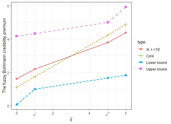
Figure 2 shows the AI of the fuzzy Bühlmann credibility for $\lambda=1 / 2$ as well as the core, lower and upper bounds of the credibility calculated using equations (3.16), (3.17) and (3.18). As discussed in Remark 3.4 , the bounds actually coincide with those derived in Hong and Martin (2021).

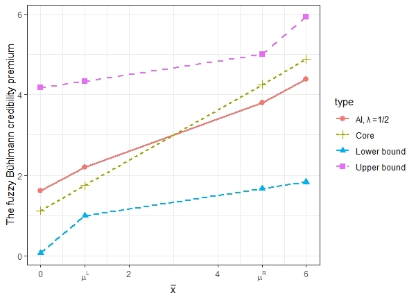
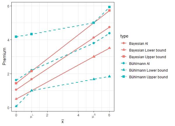
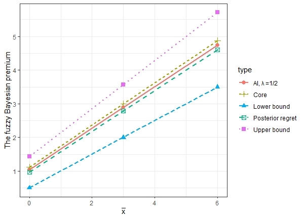
Figure 3 shows the bounds of the fuzzy Bayesian premium and the fuzzy Bühlmann credibility premium, as well as the premium levels with $\lambda$=1/2. We notice that the spread of the bounds of the fuzzy Bühlmann credibility premium are much wider than that of the fuzzy Bayesian. However, the premiums determined by AI with $\lambda$=1/2 are comparable.

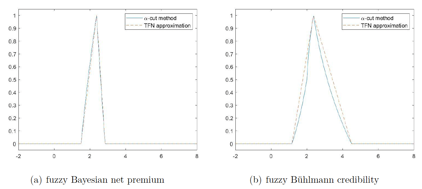
To evaluate the accuracy of the TFN approximation, we set $n=5$ and $\bar{x}=2$ and compute the fuzzy Bayesian and Bühlmann credibility premium using the $\alpha$-cut methods by applying equations (4.1) and (4.4) and compare them with the TFN approximation in (4.3) and (4.5). The results in Figure 4 illustrate that the approximation methods provide quite reasonable results.

4.2. Real data example 1

Consider the automobile insurance claim number data in Example 18.6 of Klugman, Panjer, and Willmot (2019), which includes loss experiences of 1875 policyholders over one year. The data is included in Table 1. Our goal is to use the data to estimate the parameter value of the fuzzy numbers used in fuzzy Bayesian and fuzzy credibility premium, and then use them to predict the policyholders’ expected number of losses next year.

Let’s first consider the fuzzy Bayesian credibility method. Assume that conditional on an individual’s risk parameter $\Theta=\theta$, the number of losses in a year follows a Poisson distribution with mean $\theta$. Assume that $\Theta$ follows a Gamma$(a,b)$ distribution with p.d.f. $f(x)=(b^ax^{a-1}e^{-bx})/\Gamma(a)$. However, the values of $a$ and $b$ are not known with certainty and represented by TFNs $\tilde{a}$ and $\tilde{b}$, respectively.

Following Buckley and Qu (2005), we could elicit the membership function of $\tilde{a}$ and $\tilde{b}$ by making use of the confidence intervals of ${a}$ and ${b}$. For example, we can use

$$\small{ \tilde{a}=\operatorname{TFN}\left(\hat{a}-z_{(1-\alpha / 2)} S E(\hat{a}), \hat{a}, \hat{a}+z_{(1-\alpha / 2)} S E(\hat{a})\right) \tag{4.6}}$$

and

$$\small{ \tilde{b}=T F N\left(\hat{b}-z_{(1-\alpha / 2)} S E(\hat{b}), \hat{b}, \hat{b}+z_{(1-\alpha / 2)} S E(\hat{b})\right) \tag{4.7}}$$

where $\hat{a}$ and $\hat{b}$ are point estimates of $a$ and $b$; $\alpha$ is a small probability level, such as $0.05$ or $0.01$; and $z_{(1-\alpha/2)}$ is the $(1-\alpha/2)$th quantile of a standard normal distribution.

For this Poisson-Gamma model, it is well known that $X$ follows a Negative Binomial distribution $NB(a, b)$, with probability mass function (p.m.f.)

$$\small{\begin{aligned} P(X=k)=\begin{pmatrix} k+a-1 \\ a-1\end{pmatrix}\left(\frac{1}{b+1}\right)^k \left(\frac{b}{b+1}\right)^a , \ \ k=0, 1, 2 \ldots \end{aligned}}$$

Then the log-likelihood function for the $n$ observations is simply

$$\begin{align} l(a, b)&= \sum_{i=1}^n \log (\Gamma(x_i+a))-\sum_{i=1}^n \log(\Gamma(x_i+1))\\ &\quad-n \log(\Gamma(a))+\sum_{i=1}^n x_i \log\left(\frac{1}{b+1}\right)\\ &\quad+na \log\left(\frac{b}{b+1}\right)\,. \end{align}$$

Therefore, the values of $a$ and $b$ can be estimated by MLE method. Using the R software package “maxLik” (Henningsen and Toomet 2010), we obtain $\hat{a}=1.3096$ and $\hat{b}=6.7462$, with the corresponding standard errors $SE(\hat{a})=0.2803$ and $SE(\hat{b})=1.4460$.

Applying (4.6) and (4.7) with $\alpha=0.01$, we have

$$\tilde{a}=TFN(0.5229,\, 1.3096 ,\, 2.0963)\,,$$

and

$$\tilde{b}=TFN(2.6872,\, 6.7462,\, 10.8051)\,.$$

Consequently,

$$\tilde{Z}_B=\frac{n}{\tilde{b}+n}\approx TFN(0.0847,\,0.1291,\,0.2712)\,,$$

and

$$\tilde{\mu}_B=\frac{\tilde{a}}{\tilde{b}}\approx TFN(0.0484,\,0.1941,\,0.7801)\,.$$

Then the fuzzy Bayesian premium can be calculated by applying Proposition 3.1.

Table 2 reports the calculated fuzzy Bayesian premium and the corresponding AI values. Note that the classical Bayesian premium $P_{B}(\pi_\mathbf{x})$ is given by the core of the fuzzy Bayesian premium and the imprecise credibility premium proposed by Hong and Martin (2021) is given by the bounds. For comparison, we also report the posterior regret $\Gamma$-minimax premium $RP(\pi_\mathbf{x})$ proposed in Gómez-Déniz (2009), which is simply the average of two bounds.

Now, we consider the fuzzy Bühlmann credibility. Since we only have loss data for one time period, pure non-parametric empirical Bayesian method cannot be applied to estimate parameters $\mu$, $v$ and $w$ for Bühlmann credibility premium computation. Here, to illustrate our methodology, we simply utilize the estimated $\tilde{a}$ and $\tilde{b}$ above to infer the values of $\tilde{\mu}$, $\tilde{v}$ and $\tilde{w}$. In this case, we have

$$\tilde{\mu}=\tilde{v}=\frac{\tilde{a}}{\tilde{b}}\approx TFN(0.0484,\, 0.1941,\, 0.7801)\,,$$ and $$\tilde{w}=\frac{\tilde{a}}{\tilde{b}^2}\approx TFN(0.0045,\, 0.0288,\, 0.2903)\,.$$

Consequently,

$$\tilde{k}=\frac{\tilde{v}}{\tilde{w}}\approx TFN(0.1667,\, 6.7462,\, 174.1691)\,,$$

$$\tilde{Z}_C= \frac{1}{1+\tilde{k}}\approx TFN(0.0057,\, 0.1291,\, 0.8571)\,,$$

and the fuzzy Bühlmann credibility premium can be calculated by applying Proposition 3.2.

The fuzzy Bühlmann credibility, the corresponding AI values, as well as the posterior regret $\Gamma$-minimax premium are provided in Table 3. Again, the traditional Bühlmann credibility premium is given by the core of the fuzzy Bühlmann credibility, the imprecise credibility premium studied in Hong and Martin (2021) corresponds to the bounds and the average of the bounds gives the posterior regret $\Gamma$-minimax premium.

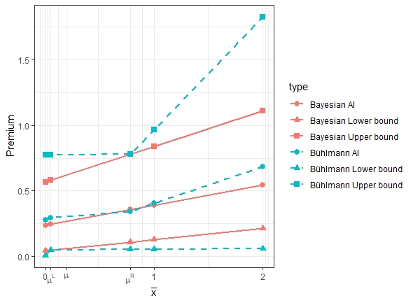
Figure 5 compares the fuzzy Bayesian premium and the fuzzy Bühlmann credibility premium. We observe that the fuzzy Bühlmann credibility has a much wider range than the fuzzy Baysian premium. This can be explained by the fact that the assumptions of Bühlmann credibility method are less restrictive than Bayesian credibility method, thus can encompass more model uncertainty.

We can also observe that, for the fuzzy Bühlmann credibility method we proposed, the credibility assigned to loss data may change based on the value of average loss experience $\bar{x}$ and the prior assumed bounds $(\mu^L, \mu^R)$. For example, $\bar{x}>\mu^R$ may indicate that the prior upper bound for $\tilde{\mu}$ is too small and not credible, thus, in determining the upper bound of the fuzzy premium, less weight is given to the prior bounds and more go to the loss experience. This explains the steeper slope of the upper bound of the Bühlmann credibility premium when $\bar{x}>\mu^R$.

4.3. Real data example 2

In this section, we consider a workers’ compensation insurance dataset that originated from the National Council on Compensation Insurance. The dataset includes loss experiences for $r=121$ occupation classes over 7 years. It was examined in Klugman (1992) using Bayesian credibility and analyzed in Frees, Young, and Luo (2001) using panel data regression models. Here we apply Bühlmann-Straub credibility method (eg. Klugman, Panjer, and Willmot 2019) to predict the losses per dollar of PAYROLL (pure premium) for every occupational class. However, we assume that there are uncertainties about the estimated parameters. Therefore, we provide the pure premium using fuzzy Bühlmann credibility theory developed in Section 3.2.

Assume that occupation class $i$ is observed for $n_i$ years and the loss exposure (PAYROLL) of class $i$ in year $j$ is denoted by $m_{ij}$. Then the total loss exposure for group $i$ over all years is given by $$m_i=\sum_{j=1}^{n_i} m_{ij}\,,$$ and the total exposure for all occupation classes and over all years is $$m=\sum_{i=1}^{r} m_{i}\,.$$ Let the experienced loss per exposure for group $i$ in year $j$ be denoted by $x_{ij}$, then its average loss per exposure over all years is $$\bar{x}_i=\frac{\sum_{j=1}^{n_i}m_{ij}x_{ij}}{m_i}\,,$$ and the average over all classes and year is $$\bar{x}=\frac{\sum_{i=1}^{j}m_{i}\bar{x}_{i}}{m}\,.$$

Applying the Bühlmann-Straub credibility formulas (see for example, Klugman, Panjer, and Willmot 2019), the predicted loss per exposure (pure premium) of class $i$ is given by $$\hat{P}_i=\hat{Z}_i \bar{x}_i+(1-\hat{Z}_i)\hat{\mu}\,,$$ where $$\hat{Z}_i= \frac{m_i}{m_i+\hat{k}}\,,$$ $\hat{k}=\hat{v}/\hat{w}$, and $$\hat{\mu}=\frac{\sum_{i=1}^r \sum_{j=1}^{n_i} m_{ij}x_{ij}}{m},$$ $$\hat{v}=\frac{\sum_{i=1}^r \sum_{j=1}^{n_i} m_{ij}(x_{ij}-\bar{x}_i)^2}{\sum_{i=1}^r(n_i-1)},$$ and $$\hat{w}=\frac{\sum_{i=1}^r m_i(\bar{x}_i-\bar{x})^2-\hat{v}(r-1)}{m-m^{-1}\sum_{i=1}^rm_i^2}.$$ For the dataset, with PAYROLL in millions, we obtain $\hat{\mu}= 0.0087$, $\hat{v}=0.0076$, and $\hat{w}= 0.000078$.

Now, we suppose that there is uncertainty/ambiguity about these parameter values and that different actuaries have different expert opinions about these values. In this case, we can consider a fuzzy Bühlmann credibility solution.

For instance, we may suppose that the credibility parameters are TFNs $\tilde{\mu}$, $\tilde{v}$ and $\tilde{w}$ with cores $\hat{\mu}$, $\hat{v}$ and $\hat{w}$, respectively. For their bounds, we applied a method introduced in Hong and Martin (2020), which assumed that the parameter’s fuzzy upper bound is given by multiplying the core value by a so-called imprecision factor $\phi>1$ and the lower bound by dividing the core value by $\phi$.

For illustration, we arbitrarily choose $\phi = 2$ and obtain

$$\begin{aligned} \tilde{\mu}=TFN(\phi^{-1}\hat{\mu}, \,\hat{\mu},\, \phi\hat{\mu})=TFN(0.0044,\, 0.0087,\, 0.0175)\,, \end{aligned}$$

$$\tilde{v}=TFN(\phi^{-1}\hat{v}, \,\hat{v},\, \phi\hat{v})=TFN(0.0038,\, 0.0076,\, 0.0151)\,,$$

and

$$\begin{align} \tilde{w}&=TFN(\phi^{-1}\hat{w}, \,\hat{w},\, \phi\hat{w})\\ &=TFN(0.000035,\, 0.000078,\, 0.000151)\,. \end{align}$$

Consequently,

$$\begin{align} \tilde{k}&=\frac{\tilde{v}}{\tilde{w}}\approx TFN(24.1406,\, 96.5623,\, 386.2494)\,, \end{align}$$

$$\tilde{Z}_i= \frac{m_i}{m_i+\tilde{k}}\,,$$

and the fuzzy Bühlmann credibility premium can be calculated by applying the results in Proposition 3.3.

We emphasize that the triangular fuzzy membership and the bounds values are arbitrarily selected here for illustration purposes. In practice, they could be decided considering the weights that are assigned to different opinions.

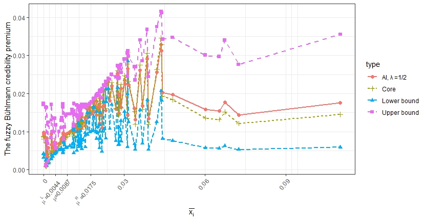
To illustrate the results, we calculate the fuzzy credibility pure premium for all occupational classes. The results are shown in Figure 6.

Since different occupational classes have different exposures, it becomes difficult to generalize the relationship between loss experience and the predicted pure premium. However, one may conclude that two situations can contribute to larger distances between the upper and lower bounds: (1) when the loss exposure is small, which indicates that the loss experience is not credible; and (2) when the loss experiences are outside the range of hypothetical mean $\left(\bar{x}_i<\mu^L\right.$, or $\left.\bar{x}_i>\mu^R\right)$, which cast doubts on the hypothetical mean.

In addition, recall that the traditional Bühlmann credibility premium is given by the core. The reported AI values are based on the arbitrarily chosen value of $\lambda=1/2$. In practice, the values can be adjusted according to the user’s preferences, as discussed after Definition 2.7.

5. Conclusions

Fuzzy set theory aims at modeling imprecise, incomplete or vague information and/or subjectivity in decision making in a formal and mathematically rigorous way. As pointed out in Shapiro (2004), fuzzy set theory have been applied in many insurance areas. In this paper, we propose to apply the theory to study the actuarial credibility theory when there are uncertainty about the loss model or the prior distribution of risk parameters. Both Bayesian and Bühlmann credibility methods are considered. Our results generalize those in Gómez-Déniz (2009), which applied posterior regret $\Gamma$-minimax principle, and those in Hong and Martin (2021), which applied imprecise probability method. We note that Koissi and Shapiro (2012) discussed the concept of credibility of a fuzzy set, which is based on the possibility and necessity measure of fuzzy sets (Liu 2007). This concept is different from the actuarial credibility theory. However, as noted in Koissi and Shapiro (2012), there are connections, and the former could find applications in solving actuarial problems. This could be a future research topic.

---

Acknowledgment

The second author of the paper gratefully acknowledges the financial support of the Natural Sciences and Engineering Research Council (NSERC) of Canada, grant number RGPIN-2019-06561.